A mathematical formulation of the Mahaux-Weidenmüller formula for the scattering matrix

1. Introduction

The purpose of this paper is to give a mathematical explanation of a formula for the scattering matrix for a manifold with infinite cylindrical ends or a waveguide. This formula, which is well known in the physics literature, is sometimes referred to as the Mahaux-Weidenmüller formula [9]. We show that a version of this formula given in (1.9) below gives the standard scattering matrix used in the mathematics literature. We also show that the finite rank approximation of the interaction matrix gives an approximation of the scattering matrix with errors inversely proportional to a fixed dimension-dependent power of the rank.

Theorem 1.

Let $X=X_{0}\cup(0,\infty)\times\partial{X_{0}}$ be a manifold with cylindrical ends – see §2 for a precise definition and Figure 1 for an illustration. Let $\{\Psi_{n}\}_{n=0}^{\infty}$ be an orthonormal set of real eigenfunctions of the Neumann Laplacian, $-H_{\rm{in}}$, on $X_{0}$ with eigenvalues $-\tau_{n}^{2}$. Let $\{\varphi_{\lambda}\}$ be the same set for the Laplacian on $\partial X_{0}$, with $-\sigma_{\lambda}^{2}$ denoting the corresponding eigenvalues. Let us define the interaction matrix by

(1.3) $$\begin{gathered}W_{N,\Lambda}(k)\;:\;L^{2}(\partial X_{0})\longrightarrow L^{2}(X_{0})\,,\\ W_{N,\Lambda}f=\sum_{0\leq\tau_{n}\leq\sqrt{N}}\Psi_{n}\sum_{0\leq\sigma_{\lambda}\leq\sqrt{\Lambda}}(k^{2}-\sigma_{\lambda}^{2})^{\frac{1}{4}}\langle\Psi_{n}\!\!\upharpoonright_{\partial X_{0}},\varphi_{\lambda}\rangle\langle f,\varphi_{\lambda}\rangle\,,\end{gathered}$$

and the effective Hamiltonian by

$$H_{N,\Lambda}(k)\stackrel{{\scriptstyle\rm{def}}}{{=}}H_{\rm{in}}-iW_{N,\Lambda}(k)W_{N,\Lambda}(k)^{t}\,.$$

Then for $k\in{\mathbb{R}}$, the entries of the scattering matrix (see §2) are given by $S_{\lambda,\lambda^{\prime}}(k)=\;$

(1.4) $$-\langle(I-2iW_{N,\Lambda}(k)^{t}(k^{2}-H_{N,\Lambda}(k))^{-1}W_{N,\Lambda}(k))\varphi_{\lambda^{\prime}},\varphi_{\lambda}\rangle+{\mathcal{O}}(N^{-\frac{1}{2}}+e^{-\Lambda/C})\,,$$

if $\sigma_{\lambda},\sigma_{\lambda^{\prime}}\leq|k|$, and $\Lambda>k^{2}$. The error bound ${\mathcal{O}}(N^{-\frac{1}{2}})$ is optimal – see §6, and the constant can be chosen uniformly for $k$ lying in compact sets.

Theorem 2 provides a related result, for other values of $k$. Also, we remark that the matrix defined by the leading term in (1.4), $\sigma_{\lambda},\sigma_{\lambda^{\prime}}\leq|k|$, is in fact unitary – see Lemma 5.1.

The physics literature contains several versions of the Mahaux-Weidenmüller formula. One commonly found formula – see for instance [1],[11] and references given there – is given as follows

(1.5) $$\widetilde{S}_{f}(k)=-\left(I-2iW(k)^{*}(k^{2}-\widetilde{H}_{\rm{eff}})^{-1}W(k)\right).$$

Here

(1.6) $$\widetilde{H}_{\rm{eff}}\stackrel{{\scriptstyle\rm{def}}}{{=}}H_{\rm{in}}-iW(k)W(k)^{*}$$

where $-H_{\rm{in}}$ is the Neumann Laplacian in the “interaction region” $X_{0}$, a compact piece of the waveguide or manifold with infinite cylindrical end, and $W(k)$ is the frequency dependent interaction matrix. When applied in numerical simulations only finite number of modes of $H_{\rm{in}}$ are taken which results in a finite rank approximation of $W(k)$, as described in (1.3). The formula, in its finite rank version, is the basis of random matrix models in scattering theory – see [6, Section III.D]. For some recent experimental results related to the formula see for instance [14].

The formula (1.5) is not strictly speaking correct. The advantage of (1.5) is that $\widetilde{S}_{f}(k)$ is unitary for real $k$ by a linear algebra argument. It is also close to the correct scattering matrix given below.

As shown in Proposition 3.5, the scattering matrix [2] which is standard in the mathematical literature is recovered from an expression close to (1.5):

(1.7) $$S_{f}(k)=-\left(I-2iW(k)^{t}(k^{2}-H_{\rm{eff}})^{-1}W(k)\right)$$

with

(1.8) $$H_{\rm{eff}}=H_{\rm{in}}-iW(k)W(k)^{t}\,,$$

and, with the notation of (1.3),

$$W(k)\stackrel{{\scriptstyle\rm{def}}}{{=}}W_{\infty,\infty}(k)\,.$$

In fact, $-H_{\operatorname{eff}}=-H_{\operatorname{eff}}(k)$ is the Laplacian on $X_{0}$, with a boundary condition that depends on $k$; see Lemma 3.2. Lemma 3.3 demonstrates the relationship between $(k^{2}-H_{\operatorname{eff}})^{-1}$ and the resolvent of the Laplacian on $X$.

This correct version (1.7) appears in [1], though again only a finite number of modes are included. We note that our sign convention, while agreeing with [1], is not consistent with many other authors. It appears that this sign is correct, and that the difference can be traced to a different normalization of the scattering matrix. The difference between (1.5) and (1.7) does not appear in many of the physics papers, where generally only an approximation $W_{a}(k)$ of $W(k)$ is used, and the approximation is such that $W_{a}(k)^{*}=W_{a}(k)^{t}$. The operator $S_{f}(k)$, unlike $\widetilde{S}_{f}(k)$, is typically not unitary for real $k$.

However, (1.7) gives what one might call the extended, or full, scattering matrix. To get the usual finite dimensional unitary scattering matrix (whose dimension changes at roots of the eigenvalues of the cross section of the end), we put, for $k$ real,

(1.9) $$S(k)=-\Pi_{k^{2}}^{\partial X_{0}}\left(I-2iW(k)^{t}(k^{2}-H_{\rm{eff}})^{-1}W(k)\right)\Pi_{k^{2}}^{\partial X_{0}}$$

where $\Pi_{k^{2}}^{\partial X_{0}}$ projects to the span of the eigenfunctions of $-\Delta_{Y}$, with eigenvalue at most $k^{2}$. Here $\Delta_{Y}$ is the Laplacian on the cross section of the end. Proposition 3.5 shows that this is the unitary scattering matrix which appears in the mathematical literature. Lemma 5.1 gives an algebraic proof that the matrix given by (1.9) is unitary for $k\in{\mathbb{R}}$. Note that if $k\in{\mathbb{R}}$, the operator defined by (1.5) is unitary, but the finite rank-operator (corresponding to a finite-dimensional matrix)

$$-\Pi_{k^{2}}^{\partial X_{0}}\Big{(}I-2iW(k)^{*}(k^{2}-H_{\rm{eff}})^{-1}W(k)\Big{)}\Pi_{k^{2}}^{\partial X_{0}}$$

with $H_{\rm{eff}}$ given by (1.6), is not unitary in general, if $W(k)$ takes into account contributions of evanescent modes. Evanescent modes correspond to eigenvalues of $-\Delta_{Y}$ larger than $k^{2}$.

Let us add that the articles [1] and [11] already have a fairly mathematically careful description of the Mahaux-Weidenmüller formula. In [12] a detailed analysis of several one dimensional models is also provided. Another related approach to scattering/transport is due to Fisher-Lee [5], see also [3].

Acknowledgments. We would like to thank Stéphane Nonnenmacher for encouraging us to write this paper, Henning Schomerus for letting us know about the Fisher-Lee formalism, Ulrich Kuhl for helpful conversations, and an anonymous referee whose comments helped us to clarify the exposition. Part of the work on this note was done while the first author was a visitor at MSRI. The partial support of the work of the first author by MSRI, an MU research leave, and the NSF grant DMS 0500267 is gratefully acknowledged, as is that of the second author by the NSF grant DMS 0654436. The first author thanks the Mathematics Department of U.C. Berkeley for its hospitality in spring 2009.

Remark. We use the notation $(u,v)$ to denote the Hermitian inner product, and $\langle u,v\rangle$ to denote the form which is linear in both arguments.

2. Scattering matrix

In this section we recall the general assumptions for manifolds with cylindrical ends and the definition of the scattering matrix.

Figure 1. An example of a manifold with an infinite cylindrical end.

Our model is a manifold $X$ with infinite cylindrical ends and smooth metric $g$– see Figure 1. In physics language that means a waveguide with periodic boundary conditions. The same arguments apply to waveguides with Dirichlet or Robin boundary condition but we choose to avoid mild technical complications associated with that setting. For purely notational reasons we also assume that there is only one end. Then

$$X=X_{0}\sqcup(0,\infty)\times Y\,,\ \ Y=\partial X_{0}\,,$$

where $X_{0}$ is a compact manifold with a smooth boundary $Y$. We require that $g\!\!\upharpoonright_{[0,\infty)\times Y}=(dx)^{2}+g_{Y}$, where $g_{Y}$ is a metric on $Y$. Moreover, we choose our decomposition so that there is a neighborhood $U\subset X_{0}$ of $\partial X_{0}$ on which $g$ is a also a product:

$$g\!\!\upharpoonright_{U}=(dx)^{2}+g_{Y}\,.$$

Recall that $\{\varphi_{\lambda}\}$ are an orthonormal set of eigenfunctions of $\Delta_{Y}$. We use the convention that the energy is $k^{2}$, and $k_{\lambda}=\sqrt{k^{2}-\sigma_{\lambda}^{2}}$, with the imaginary part chosen to be non-negative when $\operatorname{\rm Im}\nolimits k\geq 0$. We call the region with $\operatorname{\rm Im}\nolimits k\geq 0$ the physical region. Given $\lambda\in{\mathbb{N}}$, if $k$ is in the physical region, and with $\operatorname{\rm Im}\nolimits k>0$, there is a unique $\Phi_{\lambda}(p,k)$ so that

(2.1) $$(-\Delta_{X}-k^{2})\Phi_{\lambda}(p,k)=0\;\text{on $X$}$$

and

(2.2) $$\Phi_{\lambda}\!\!\upharpoonright_{(0,\infty)\times Y}=e^{-ik_{\lambda}x}\frac{\varphi_{\lambda}(y)}{\sqrt{k_{\lambda}}}+\sum_{\lambda^{\prime}}S_{\lambda^{\prime}\lambda}(k)e^{ik_{\lambda^{\prime}}x}\frac{\varphi_{\lambda^{\prime}}(y)}{\sqrt{k_{\lambda^{\prime}}}}$$

for some $S_{\lambda^{\prime}\lambda}$. To see this we use the resolvent $(-\Delta_{X}-k^{2})^{-1}$ which is a bounded operator $L^{2}(X)\rightarrow H^{2}(X)$, for $\operatorname{\rm Im}\nolimits k>0$:

$$\Phi_{\lambda}(p,k)=(1-\psi)\varphi_{\lambda}(y)e^{-ik_{\lambda}x}+(-\Delta_{X}-k^{2})^{-1}\left([\Delta_{X},\psi]\left(\varphi_{\lambda}(y)e^{-ik_{\lambda}x}\right)\right)(p)\,,$$

$$\psi\in C^{\infty}_{0}(X)\,,\ \ \psi\!\!\upharpoonright_{X_{0}}\equiv 1\,.$$

Since on $X_{1}$ we have $-\Delta_{X}=-\partial_{x}^{2}-\Delta_{Y}$, separation of variables shows that $\Phi_{\lambda}$ can be written as in (2.2).

The resolvent, $(-\Delta_{X}-k^{2})^{-1}$, continues meromorphically to

(2.3) $$\Lambda_{\sigma(\Delta_{\partial X_{0}})}\supset\{k\;:\;\operatorname{\rm Im}\nolimits k>0\}\,,$$

a Riemann surface branched at $\sigma_{\lambda}$’s – see [10, Sect.6.7]. We remark that this Riemann surface is such that each $k_{\lambda}$ defined above extends to be a holomorphic single-valued function. Thus $\Phi_{\lambda}(p,k)$ has a meromorphic continuation to $\Lambda_{\sigma(\Delta_{\partial X_{0}})}$ which is regular for $\operatorname{\rm Im}\nolimits k=0$ except when $k_{\lambda^{\prime}}$’s are $0$, or when $k^{2}\in\sigma(-\Delta_{X})$.

The full, or extended, scattering matrix is the infinite matrix

$$S_{f}(k)=(S_{\lambda^{\prime}\lambda}(k))_{\lambda,\lambda^{\prime}\in{\mathbb{N}}}.$$

For $k\in{\mathbb{R}}$, the matrix more commonly called the scattering matrix is the finite-dimensional matrix given by

$$S(k)=(S_{\lambda^{\prime}\lambda}(k))_{\sigma_{\lambda}^{2},\sigma_{\lambda^{\prime}}^{2}\leq k^{2}}.$$

We remark that if $\operatorname{\rm Im}\nolimits k>0$, while each entry $S_{\lambda\lambda^{\prime}}(k)$ is well-defined away from its poles, there is not a canonical choice for “the” scattering matrix. However, in general it is $(\sqrt{k_{\lambda}}/\sqrt{k_{\lambda^{\prime}}})S_{\lambda^{\prime}\lambda}(k)$, not $S_{\lambda^{\prime}\lambda}$, which has a meromorphic continuation to $\Lambda_{\sigma(\Delta_{\partial X_{0}})}$ for each $\lambda,\;\lambda^{\prime}$. We shall use this continuation in the proof of the theorem.

3. The formula

Let $\Delta_{Y}$ be the Laplacian on $Y$, and let $\{\sigma_{\lambda}^{2}\}$ be the eigenvalues of $-\Delta_{Y}$, repeated according to multiplicity, and let $\{\varphi_{\lambda}\}$ be an associated set of real, orthonormal eigenfunctions of the Laplacian on $Y$. Let $-H_{\rm{in}}$ be the Laplacian with Neumann boundary conditions on $X_{0}^{\circ}$, and let $\{\Psi_{n}\}$ be a set of real, orthonormal eigenfunctions of $H_{\rm{in}}$.

First, we define the operator $W(k)$ by explicitly giving its Schwartz kernel. Our starting point is the representation of $W(k)$ from [1] or [11]. We write $p$ to represent a point in ${X_{0}}$, and $y$ or $y^{\prime}$ to represent a point in $Y$; on $U\subset X_{0}$ we may write $p=(x,y)$, with $\{x=0\}=\partial X_{0}$. Then, with

$$\Psi_{n,\lambda}(0)\stackrel{{\scriptstyle\rm{def}}}{{=}}\int_{Y}\varphi_{\lambda}(y)\Psi_{n}(0,y)\,,$$

we follow the physics literature and define the coupling operator by giving its integral kernel (with integration with respect to Riemannian densities) as

(3.1) $$\begin{split}W(p,y^{\prime})&\stackrel{{\scriptstyle\rm{def}}}{{=}}\sum_{n,\lambda}\sqrt{{k_{\lambda}}}\Psi_{n}(p)\Psi_{n,\lambda}(0)\varphi_{\lambda}(y^{\prime})\\ &=\sum_{n}\Psi_{n}(p)P_{k}\Psi_{n}(0,y^{\prime}).\end{split}$$

Here $P_{k}=(k^{2}+\Delta_{Y})^{1/4}$ is defined by $P_{k}\varphi_{\lambda}=\sqrt{k_{\lambda}}\varphi_{\lambda}$. While either choice of the square root is possible, it is crucial that this is consistent with that used to define the scattering matrix; see (2.2). The series converges in the sense of distributions. Hence, $W(p,y^{\prime})$ is understood as a distribution on $X\times Y$ – see Lemma 3.1 below.

This definition (3.1) appears normally in the physics literature. When we take all the eigenstates then $W$ (and especially $W^{t}$) takes a very simple form given in the following lemma. When, as is done in the physics literature, we take only finitely many states, the formula for $W^{t}$ is given in the remark after the lemma.

Let $\dot{\mathcal{D}}^{\prime}(X_{0})$ be the space of distributions on $X$ supported in the (closed) set $X_{0}$. We also use the following convention: for $s\geq 0$ the space $H^{s}(X_{0})$ denotes restrictions of elements of $H^{s}(X)$ to $X_{0}$, while for $s\leq 0$, $H^{s}(X_{0})$ denotes elements of $H^{s}(X)$ supported in the (closed) set $X_{0}$. See [7, Appendix B.2] for a careful discussion: in the notation used there

$$H^{s}(X_{0})=\left\{\begin{array}[]{ll}\bar{H}_{(s)}(X_{0})&s\geq 0\\ \dot{H}_{(s)}(X_{0})&s\leq 0\,.\end{array}\right.$$

With this notation in place we can formulate

Lemma 3.1.

The operator (3.1) is equal to

(3.2) $$W(k)g=\delta_{\partial X_{0}}\,P_{k}g\,,\ \ g\in C^{\infty}(\partial X_{0})\,,$$

where $\delta_{\partial X_{0}}\in\dot{\mathcal{D}}^{\prime}(X_{0})$ is the distribution defined by

$$\delta_{\partial X_{0}}(\varphi)=\int_{\partial X_{0}}\varphi\!\!\upharpoonright_{\partial X_{0}}d{\rm{vol}}_{Y}\,.$$

We have

(3.3) $$W(k):H^{s}(Y)\rightarrow H^{\min(-1/2-,s-1)}(X_{0})\,,\ \ s\in{\mathbb{R}}\,,$$

and $W(k)g\!\!\upharpoonright_{X_{0}^{\circ}}=0$. The transpose, $W(k)^{t}:H^{1/2+s}(X_{0})\rightarrow H^{-1/2+s}(Y)$, $s>0$, is given by

(3.4) $$W(k)^{t}f(y)=P_{k}(f\!\!\upharpoonright_{\partial X_{0}})\,.$$

Proof.

To prove (3.2) we need to compute, in the notation of distributions, $W(f\otimes g)$, where $f\in\bar{C}^{\infty}_{0}(X_{0})$. The definition (3.1) gives

$$\begin{split}W(f\otimes g)&=\sum_{n}\left(\int_{X_{0}}\Psi_{n}f\right)\left(\int_{\partial X_{0}}\Psi_{n}\!\!\upharpoonright_{\partial X_{0}}P_{k}g\right)\\ &=\int_{\partial X_{0}}\left(\sum_{n}\left(\int_{X_{0}}\Psi_{n}f\right)\Psi_{n}\!\!\upharpoonright_{\partial X_{0}}\right)P_{k}g\\ &=\int_{\partial X_{0}}f\!\!\upharpoonright_{\partial X_{0}}P_{k}g\,,\end{split}$$

which proves (3.2) and, by duality, (3.4). The mapping property of $W(k)^{t}$ follows from the fact that $f\mapsto f\!\!\upharpoonright_{X_{0}}$ takes $H^{s+1/2}(X_{0})$ to $H^{s}(\partial X_{0})$ for $s>0$, and $P_{k}:H^{s}(\partial X_{0})\rightarrow H^{s-1/2}(\partial X_{0})$. The mapping property (3.3) follows by duality. ∎

Remark. In Lemma 3.1 all the structure of the the basis of eigenvectors of $H_{\rm{in}}$ and $\Delta_{Y}$ disappears. The question which we address in Section 4 is how close the approximation based on using only finitely many basis elements gets to the actual scattering matrix. Then for $a=(N,\Lambda)\in[0,\infty]^{2}$ we define

$$W_{a}(k)^{t}\stackrel{{\scriptstyle\rm{def}}}{{=}}P_{k}\,{\mathchoice{1\mskip-4.0mu{\rm{l}}}{1\mskip-4.0mu{\rm{l}}}{1\mskip-4.5mu{\rm{l}}}{1\mskip-5.0mu{\rm{l}}}}_{[0,N]}(\Delta_{Y})R\,{\mathchoice{1\mskip-4.0mu{\rm{l}}}{1\mskip-4.0mu{\rm{l}}}{1\mskip-4.5mu{\rm{l}}}{1\mskip-5.0mu{\rm{l}}}}_{[0,\Lambda]}(H_{\rm{\rm{in}}})\,,\ \ Ru\stackrel{{\scriptstyle\rm{def}}}{{=}}u\!\!\upharpoonright_{\partial X_{0}}\,.$$

We note that

$$W_{(\infty,\infty)}(k)=W(k)\,,$$

and that for $N<\infty$ and $\Lambda<\infty$,

$$W_{a}(k)\;:\;{\mathcal{D}}^{\prime}(Y)\longrightarrow C^{\infty}(X_{0})\,,\ \ W_{a}(k)^{t}\;:\;\dot{\mathcal{D}}^{\prime}(X_{0})\longrightarrow C^{\infty}(Y)\,,$$

where $C^{\infty}(X_{0})$ denotes extendable smooth functions on the compact manifold $X_{0}$.

We make the definition (1.8) of $H_{\operatorname{eff}}$ rigorous via the quadratic form

$$q(u,v) =q(k)(u,v)=\int_{X_{0}}\nabla u\overline{\nabla v}\;d{\rm vol}_{X_{0}}-i\int_{\partial X_{0}}W^{t}(k)u\overline{W^{*}(k)v}\;d{\rm vol}_{Y}$$

$$=\int_{X_{0}}\nabla u\overline{\nabla v}\;d{\rm vol}_{X_{0}}-i\int_{\partial X_{0}}P_{k}Ru\overline{P_{k}^{*}Rv}\;d{\rm vol}_{Y}$$

with form domain $H^{1}(X_{0})$. If

$$q(u,v)=(w,v)$$

for some $w\in L^{2}(X_{0})$ and all $v\in H^{1}(X_{0})$, then $u$ is in the domain of $H_{\operatorname{eff}}$ and $H_{\operatorname{eff}}u=w.$ Moreover,

$$(w,v)=q(u,v)=-\int_{X_{0}}\Delta_{X_{0}}u\overline{v}+\int_{\partial X_{0}}(\partial_{n}u-iP_{k}^{2}Ru)\overline{v}\,,$$

where $\partial_{n}u$ denotes the outward unit normal derivative at the boundary. Since this must hold for all $v\in H^{1}(X_{0})$, $-\Delta_{X_{0}}u=w$ and

$$0=\partial_{n}u-iP^{2}_{k}Ru.$$

We note that $u\in H^{2}(X_{0})$ where the space is defined by restricting elements of $H^{2}(X)$ to $X_{0}$ – see [7, Appendix B]. We summarize this in the following

Lemma 3.2.

Suppose $u\in\operatorname{Domain}(H_{\operatorname{eff}})$. Then $u\in H^{2}(X_{0})$, and

$$H_{\operatorname{eff}}u=-\Delta_{X_{0}}u\,,\ \ \partial_{n}u-iP_{k}^{2}Ru=0\,.$$

Next we investigate the relation between $(k^{2}-H_{\operatorname{eff}})^{-1}$ and the resolvent of the Laplacian on $X$. Denote

$$R_{X}(k)\stackrel{{\scriptstyle\rm{def}}}{{=}}(k^{2}+\Delta_{X})^{-1},\;\text{for $\operatorname{\rm Im}\nolimits k>0$}.$$

Then, for $K\subset X$ any compact set ${\mathchoice{1\mskip-4.0mu{\rm{l}}}{1\mskip-4.0mu{\rm{l}}}{1\mskip-4.5mu{\rm{l}}}{1\mskip-5.0mu{\rm{l}}}}_{K}R_{X}(k){\mathchoice{1\mskip-4.0mu{\rm{l}}}{1\mskip-4.0mu{\rm{l}}}{1\mskip-4.5mu{\rm{l}}}{1\mskip-5.0mu{\rm{l}}}}_{K}$ has a meromorphic extension to $\Lambda_{\sigma(\Delta_{\partial X_{0}})}$, see [10]. In Lemma 4.1 we shall show that $(k^{2}-H_{\operatorname{eff}})^{-1}:L^{2}(X_{0})\rightarrow H^{2}(X_{0})$ exists for $k^{2}\ll 0$, $\operatorname{\rm Im}\nolimits k>0$, and is meromorphic on $\Lambda_{\sigma(\Delta_{\partial X_{0}})}$, the Riemann surface (2.3). One could provide an alternate proof using the first part of the proof of Lemma 3.3 and the results of [10] on the meromorphic continuation of $R_{X}(k)$.

We remark that when we use $k\in\Lambda_{\sigma(\Delta_{\partial X_{0}})}$, by abuse of notation we mean by $k^{2}$ the complex number which is the continuation of $k^{2}$ from the physical half plane $\operatorname{\rm Im}\nolimits k\geq 0$.

Lemma 3.3.

We have the following relation between $R_{X}(k)$ as defined above and $(k^{2}-H_{\operatorname{eff}})^{-1}=(k^{2}-H_{\operatorname{eff}}(k))^{-1}$:

$$(k^{2}-H_{\operatorname{eff}})^{-1}={\mathchoice{1\mskip-4.0mu{\rm{l}}}{1\mskip-4.0mu{\rm{l}}}{1\mskip-4.5mu{\rm{l}}}{1\mskip-5.0mu{\rm{l}}}}_{X_{0}}R_{X}(k){\mathchoice{1\mskip-4.0mu{\rm{l}}}{1\mskip-4.0mu{\rm{l}}}{1\mskip-4.5mu{\rm{l}}}{1\mskip-5.0mu{\rm{l}}}}_{X_{0}}$$

for $k\in\Lambda_{\sigma(\Delta_{\partial X_{0}})}$. In particular, the poles of $(k^{2}-H_{\operatorname{eff}})^{-1}$ are the same as the poles of $R_{X}(k)$.

Proof.

Suppose $g\in L^{2}(X_{0})\subset L^{2}(X)$ and $g$ is $0$ in a neighborhood of $\partial X_{0}$. Then

(3.5) $$(k^{2}+\Delta_{X_{0}}){\mathchoice{1\mskip-4.0mu{\rm{l}}}{1\mskip-4.0mu{\rm{l}}}{1\mskip-4.5mu{\rm{l}}}{1\mskip-5.0mu{\rm{l}}}}_{X_{0}}R_{X}(k)g=(k^{2}+\Delta_{X_{0}}){\mathchoice{1\mskip-4.0mu{\rm{l}}}{1\mskip-4.0mu{\rm{l}}}{1\mskip-4.5mu{\rm{l}}}{1\mskip-5.0mu{\rm{l}}}}_{X_{0}}R_{X}(k){\mathchoice{1\mskip-4.0mu{\rm{l}}}{1\mskip-4.0mu{\rm{l}}}{1\mskip-4.5mu{\rm{l}}}{1\mskip-5.0mu{\rm{l}}}}_{X_{0}}g=g\;\text{ on $X_{0}^{\circ}$}$$

for $k\in\Lambda_{\sigma(\Delta_{\partial X_{0}})}.$

Note that since $\operatorname{supp}g\subset X_{0}$, $(k^{2}+\Delta_{X})g=0$ on $X_{1}$. Then for $\operatorname{\rm Im}\nolimits k>0$ (that is, for $k$ in the physical space), the requirement that $R_{X}(k)g\in L^{2}(X)$ means that

(3.6) $$R_{X}(k)g\!\!\upharpoonright_{X_{1}}=\sum a_{\lambda}e^{ik_{\lambda}x}\varphi_{\lambda}$$

for some constants $a_{\lambda}=a_{\lambda}(k)$. But then, using the support conditions of $g$ there is a neighborhood $\tilde{U}\subset X_{0}$ of $\partial X_{0}$ so that

$$R_{X}(k)g\!\!\upharpoonright_{\tilde{U}}=\sum a_{\lambda}e^{ik_{\lambda}x}\varphi_{\lambda}.$$

Thus

$$(\partial_{n}-iP_{k}^{2})(R_{X}(k)g\!\!\upharpoonright_{X_{0}})\!\!\upharpoonright_{\partial X_{0}}=0$$

so that $R_{X}(k)g\!\!\upharpoonright_{X_{0}}$ is in the domain of $H_{\operatorname{eff}}=H_{\operatorname{eff}}(k)$. Together with (3.5), this means that

$$(k^{2}-H_{\operatorname{eff}})^{-1}g={\mathchoice{1\mskip-4.0mu{\rm{l}}}{1\mskip-4.0mu{\rm{l}}}{1\mskip-4.5mu{\rm{l}}}{1\mskip-5.0mu{\rm{l}}}}_{X_{0}}R_{X}(k)g$$

for all $k$ with $\operatorname{\rm Im}\nolimits k>0$ and all $g\in L^{2}(X_{0})$ which are $0$ in a neighborhood of $\partial X_{0}$. Since such $g$ are dense in $L^{2}(X_{0})$, this must in fact hold for all $g\in L^{2}(X_{0})$.

Since $(k^{2}-H_{\operatorname{eff}})^{-1}={\mathchoice{1\mskip-4.0mu{\rm{l}}}{1\mskip-4.0mu{\rm{l}}}{1\mskip-4.5mu{\rm{l}}}{1\mskip-5.0mu{\rm{l}}}}_{X_{0}}R_{X}(k){\mathchoice{1\mskip-4.0mu{\rm{l}}}{1\mskip-4.0mu{\rm{l}}}{1\mskip-4.5mu{\rm{l}}}{1\mskip-5.0mu{\rm{l}}}}_{X_{0}}$ for all $k$ with $\operatorname{\rm Im}\nolimits k>0$ and since both sides have meromorphic continuations to $\Lambda_{\sigma(\Delta_{\partial X_{0}})}$ (see [10] and Lemma 4.1), they must in fact agree for all $k\in\Lambda_{\sigma(\Delta_{\partial X_{0}})}$. ∎

Lemma 3.4.

Suppose $(k^{2}-H_{\operatorname{eff}})^{-1}$ exists. For $f\in H^{1}(\partial X_{0})$, let

$$u=(k^{2}-H_{\operatorname{eff}})^{-1}W(k)f\,.$$

Then

(3.7) $$(k^{2}+\Delta_{X_{0}})u=0\;\text{on}\;X_{0}^{\circ}\,,\ \ (\partial_{n}-iP^{2}_{k})u\!\!\upharpoonright_{\partial X_{0}}=-P_{k}f.$$

Proof.

We first claim that there exists $F\in H^{2}(X_{0})$ such that

(3.8) $$(\partial_{n}-iP_{k}^{2})F\!\!\upharpoonright_{\partial X_{0}}=-P_{k}f\,.$$

In fact, for $0<h\ll 1$ define $N(h):H^{s}(\partial X_{0})\rightarrow H^{s-1}(\partial X_{0})$ as follows:

$$N(h)=\frac{1}{h}\langle I-\Delta_{\partial X_{0}}\rangle^{\frac{1}{2}}\,,\ \ \ N(h)^{-1}={\mathcal{O}}(h)\;:\;H^{s-1}(\partial X_{0})\longrightarrow H^{s}(\partial X_{0})\,.$$

Let $\chi\in C^{\infty}_{0}([0,\epsilon))$ be equal to $1$ in a small neighbourhood of $0$, with $\epsilon$ chosen so that $X_{0}\simeq(-\epsilon,0]_{x}\times\partial X_{0}$, near the boundary. We define (note that $x<0$)

$$[T(h)g](x,y)\stackrel{{\scriptstyle\rm{def}}}{{=}}\chi(-x)\exp(x\langle I-\Delta_{\partial X_{0}}\rangle^{\frac{1}{2}}/h)g(y)\,,$$

$$T(h)\;:\;H^{s}(\partial X_{0})\rightarrow H^{s+\frac{1}{2}}(X_{0})\,,\ \ s\geq 0\,,$$

so that

$$T(h)g\!\!\upharpoonright_{\partial X_{0}}=g\,,\ \ \partial_{n}T(h)g\!\!\upharpoonright_{\partial X_{0}}=N(h)g\,.$$

For a fixed $k$, $P_{k}^{2}={\mathcal{O}}(1):H^{3/2}(\partial X_{0})\rightarrow H^{1/2}(\partial X_{0})$, and hence, if $h$ is small enough, we have the following inverse

$$(N(h)-iP_{k}^{2})^{-1}=N(h)^{-1}(I-iP_{k}^{2}N(h)^{-1})^{-1}\;:\;H^{\frac{1}{2}}(\partial X_{0})\longrightarrow H^{\frac{3}{2}}(\partial X_{0})\,.$$

Using this and the mapping properties of $T(h)$ we construct

$$F\stackrel{{\scriptstyle\rm{def}}}{{=}}-T(h)(N(h)-iP_{k}^{2})^{-1}P_{k}f\in H^{2}(X_{0})\,,$$

which satisfies (3.8).

We now set

$$v=F-(k^{2}-H_{\operatorname{eff}})^{-1}(k^{2}+\Delta_{X_{0}})F\,,$$

and observe that $v$ satisfies the equations (3.7). It remains to show that $v=u$.

To see that we let $h\in C^{\infty}(X_{0})$, and apply Green’s formula to compute

$$((k^{2}-H_{\operatorname{eff}})^{-1}(k^{2}+\Delta_{X_{0}})F,h) =((k^{2}+\Delta_{X_{0}})F,((k^{2}-H_{\operatorname{eff}})^{-1})^{*}h)$$

$$=\int_{\partial X_{0}}\left(\partial_{n}F\overline{((k^{2}-H_{\operatorname{eff}})^{-1})^{*}h}-F\overline{\partial_{n}((k^{2}-H_{\operatorname{eff}})^{-1})^{*}h}\right)$$

$$\ \ \ +(F,(k^{2}+\Delta_{X_{0}})((k^{2}-H_{\operatorname{eff}})^{-1})^{*}h)$$

$$=\int_{\partial X_{0}}\left(\partial_{n}F\overline{((k^{2}-H_{\operatorname{eff}})^{-1})^{*}h}-F\overline{\partial_{n}((k^{2}-H_{\operatorname{eff}})^{-1})^{*}h}\right)$$

$$\ \ \ +(F,h)\,.$$

Now we use that $\partial_{n}F\!\!\upharpoonright_{\partial X_{0}}=iP_{k}^{2}(F\!\!\upharpoonright_{\partial X_{0}})-P_{k}f$, and that

$$w\in H^{2}(X_{0})\cap\operatorname{Domain}((k^{2}-H_{\operatorname{eff}})^{*})\ \Longrightarrow\ \partial_{n}w\!\!\upharpoonright_{\partial X_{0}}+i(P_{k}^{2})^{*}Rv=0\,.$$

Thus we have

$$((k^{2}-H_{\operatorname{eff}})^{-1}(k^{2}+\Delta_{X_{0}})F,h)$$

$$=\int_{\partial X_{0}}\left((iP^{2}_{k}(F\!\!\upharpoonright_{\partial X_{0}})-P_{k}f)\overline{((k^{2}-H_{\operatorname{eff}})^{-1})^{*}h}-iF\overline{((P_{k}^{2})^{*}(k^{2}-H_{\operatorname{eff}})^{-1})^{*}h}\right)+(F,h)$$

$$=-\int_{\partial X_{0}}P_{k}f\overline{((k^{2}-H_{\operatorname{eff}})^{-1})^{*}h}+(F,h)=\int_{X_{0}}\left(-(k^{2}-H_{\operatorname{eff}})^{-1}\delta_{X_{0}}P_{k}f+F\right)\bar{h}\,,$$

where the last expression follows from the definition of $\delta_{\partial{X_{0}}}$. Since this holds for all $h\in C^{\infty}(X_{0})$,

$$v=F-(k^{2}-H_{\operatorname{eff}})^{-1}(k^{2}+\Delta_{X_{0}})F=(k^{2}-H_{\operatorname{eff}})^{-1}\delta_{X_{0}}P_{k}f=u\,,$$

proving the lemma. ∎

We can now state and prove the main result of this section. It provides a justification of (1.7) and (1.9).

Proposition 3.5.

Let $W$ be given by (3.1). Then the $\lambda\lambda^{\prime}$ entry of the scattering matrix defined in §2 is given by

(3.9) $$S_{\lambda,\lambda^{\prime}}(k)=\langle S_{f}(k)\varphi_{\lambda},\varphi_{\lambda^{\prime}}\rangle_{L^{2}(\partial X_{0})}\,,$$

where

$$S_{f}(k)=-\left(I-2iW(k)^{t}(k^{2}-H_{\rm{eff}})^{-1}W(k)\right)\,,$$

and $H_{\rm{eff}}$ is defined in Lemma 3.2.

Proof.

We use Lemma 3.7 to express the action of $(k^{2}-H_{\operatorname{eff}})^{-1}W(k)$. Suppose $v_{\lambda}=(k^{2}-H_{\operatorname{eff}})^{-1}W(k)\varphi_{\lambda}.$ Let $U\subset X_{0}$ be a neighborhood of $\partial X_{0}$. On $U$ we may use coordinates $(x,y)$, with $y\in Y$. Since $v_{\lambda}$ lies in the null space of $-\Delta_{X_{0}}-k^{2}$, we have that

$$v_{\lambda}\!\!\upharpoonright_{U}=\sum_{\lambda^{\prime}}(a_{\lambda^{\prime}}e^{ik_{\lambda^{\prime}}x}+b_{\lambda^{\prime}}e^{-ik_{\lambda^{\prime}}x})\varphi_{\lambda^{\prime}}(y).$$

The boundary conditions (3.7) applied to $v_{\lambda}$ at $\partial X_{0}$ mean that

$$\sum_{\lambda^{\prime}}ik_{\lambda^{\prime}}(a_{\lambda^{\prime}}-b_{\lambda^{\prime}})\varphi_{\lambda^{\prime}}-i\sum_{\lambda^{\prime}}k_{\lambda^{\prime}}(a_{\lambda^{\prime}}+b_{\lambda^{\prime}})\varphi_{\lambda^{\prime}}=-P_{k}\varphi_{\lambda}.$$

Then $b_{\lambda}=1/({2i}{\sqrt{k_{\lambda}}})$ and $b_{\lambda^{\prime}}=0$ if $\lambda^{\prime}\not=\lambda$. Thus $v_{\lambda}$ is the restriction to $X_{0}$ of ${-i}\Phi_{\lambda}/2$, where $\Phi_{\lambda}$ is determined by (2.1) and (2.2):

(3.10) $$\Phi_{\lambda}\!\!\upharpoonright_{(0,\infty)\times Y}=e^{-ik_{\lambda}x}\frac{\varphi_{\lambda}(y)}{\sqrt{k_{\lambda}}}+\sum_{\lambda^{\prime}}S_{\lambda^{\prime}\lambda}e^{ik_{\lambda^{\prime}}x}\frac{\varphi_{\lambda^{\prime}}(y)}{\sqrt{k_{\lambda^{\prime}}}}\,.$$

Therefore

$$W(k)^{t}v_{\lambda} =\sum_{\lambda^{\prime}}\sqrt{k_{\lambda^{\prime}}}a_{\lambda^{\prime}}\varphi_{\lambda^{\prime}}-\frac{i}{2}\varphi_{\lambda}=-\frac{i}{2}\left(\sum_{\lambda^{\prime}}S_{\lambda^{\prime}\lambda}\varphi_{\lambda^{\prime}}+\varphi_{\lambda}\right)\,,$$

which proves the proposition. ∎

The equation (3.9) is valid for all real values of $k$ (that is, $k$ on the boundary of the physical space) with $k^{2}>\sigma_{\lambda}^{2},\;\sigma_{\lambda^{\prime}}^{2}$, since the matrix coming from the right hand side is unitary and hence the singularities of $\langle S_{f}(k)\varphi_{\lambda^{\prime}},\varphi_{\lambda}\rangle_{L^{2}(\partial X_{0})}$ resulting from poles of $(H_{\rm{eff}}-k^{2})^{-1}$ are removable.

4. Accuracy of Approximations

Here we investigate the accuracy of the approximations made to use (1.7) in numerical computations. Set

$$\Pi^{\partial X_{0}}_{\Lambda}f \stackrel{{\scriptstyle\rm{def}}}{{=}}{\mathchoice{1\mskip-4.0mu{\rm{l}}}{1\mskip-4.0mu{\rm{l}}}{1\mskip-4.5mu{\rm{l}}}{1\mskip-5.0mu{\rm{l}}}}_{[0,\Lambda]}(-\Delta_{\partial X_{0}})f\ \ \text{for $f\in L^{2}(\partial X_{0})$,}$$

$$\Pi^{\rm{in}}_{N}g \stackrel{{\scriptstyle\rm{def}}}{{=}}\ {\mathchoice{1\mskip-4.0mu{\rm{l}}}{1\mskip-4.0mu{\rm{l}}}{1\mskip-4.5mu{\rm{l}}}{1\mskip-5.0mu{\rm{l}}}}_{[0,N]}(H_{{\rm in}})g\ \ \text{for $g\in L^{2}(X_{0})$}.$$

In parallel with this, we introduce

$$W_{\infty,\infty}(k) \stackrel{{\scriptstyle\rm{def}}}{{=}}W(k)\,,\ \ \ W_{\infty,\Lambda}(k)\stackrel{{\scriptstyle\rm{def}}}{{=}}W\Pi^{\partial X_{0}}_{\Lambda}\,,$$

$$W_{N,\Lambda}(k) \stackrel{{\scriptstyle\rm{def}}}{{=}}\Pi^{\rm{in}}_{N}W(k)\Pi^{\partial X_{0}}_{\Lambda}=\Pi^{\rm{in}}_{N}W_{\infty,\Lambda}(k)\,,$$

and

$$H_{\infty,\infty} \stackrel{{\scriptstyle\rm{def}}}{{=}}H_{\operatorname{eff}}\,,\ \ \ H_{N,\Lambda}\stackrel{{\scriptstyle\rm{def}}}{{=}}H_{in}-iW_{N,\Lambda}W_{N,\Lambda}^{t},\;N\in{\mathbb{R}}\cup\{\infty\}\,.$$

Although $W_{N,\Lambda}$, $W_{\infty,\Lambda}$ depend on $k$, for simplicity we generally omit this in our notation. Note that $H_{\operatorname{eff}}$, $H_{\infty,\Lambda}$ and $H_{N,\Lambda}$ also depend on $k$. A quadratic form argument (see Lemmas 3.2 and 4.4), using the form domain $H^{1}(X_{0})$, shows that if $u$ is in the domain of $H_{\infty,\Lambda}$, then $\partial_{n}u-iP_{k}^{2}\Pi^{\partial X_{0}}_{\Lambda}Ru=0$. However, for $N<\infty$ the domain of $H_{N,\Lambda}$ is the set of elements of $H^{2}(X_{0})$ which satisfy the Neumann boundary condition, $\partial_{n}u=0$.

Likewise, we define the approximations of the (full) scattering matrix obtained by using the approximation $H_{N,\Lambda}$ of $H_{\operatorname{eff}}$ by $S_{f,N,\Lambda}$:

(4.1) $$S_{f,N,\Lambda}(k)=-\Big{(}I-2iW_{N,\Lambda}(k)^{t}(k^{2}-H_{N,\Lambda})^{-1}W_{N,\Lambda}(k)\Big{)}\,.$$

In order to bound the error in these approximations, we shall first see how close $\Pi^{\partial X_{0}}_{\Lambda_{0}}S_{f,\infty,\Lambda}$ is to $\Pi^{\partial X_{0}}_{\Lambda_{0}}S_{f,\infty,\infty}$, and then study the difference

$$\Pi^{\partial X_{0}}_{\Lambda_{0}}\left(S_{f,\infty,\Lambda}-S_{f,N,\Lambda}\right)\Pi^{\partial X_{0}}_{\Lambda_{0}}\,.$$

4.1. Projection on $\partial X_{0}$

We first analyze the approximation with a finite $\Lambda$ and $N=\infty$. The spectral cutoff for the boundary Laplacian, $\Lambda$ has to be taken large enough to guarantee that $\operatorname{\rm Im}\nolimits k_{\lambda}>0$ for $\sigma_{\lambda}^{2}>\Lambda$. The errors then come from evanescent modes and can be estimated using exponential decay. We present the results in two lemmas.

Recall that $H_{\operatorname{eff}}=H_{\operatorname{eff}}(k)$ is defined for $k\in\Lambda_{\sigma(\Delta_{\partial X_{0}})}$.

Lemma 4.1.

Let $\Lambda_{\sigma(\Delta_{\partial X_{0}})}$ be the Riemann surface, given in (2.3), to which the resolvent of $-\Delta_{X}$, $(-\Delta_{X}-k^{2})^{-1},$ has a meromorphic continuation (see [10, Sect.6.7]). Then the operators $(k^{2}-H_{\rm{eff}})^{-1}$ and $(k^{2}-H_{\infty,\Lambda})^{-1}$ are meromorphic on $\Lambda_{\sigma(\Delta_{\partial X_{0}})}$. If $k^{2}-H_{\operatorname{eff}}=k^{2}-H_{\operatorname{eff}}(k)$ is invertible, so is $k^{2}-H_{\infty,\Lambda}(k)$ for $\Lambda>\Lambda_{0}(k_{0})$ sufficiently large, and

$$\|(k^{2}-H_{\rm{eff}})^{-1}-(k^{2}-H_{\infty,\Lambda})^{-1}\|_{L^{2}\rightarrow L^{2}}\leq C\Lambda^{-1/2}\,,\ \ \Lambda>\Lambda_{0}(k)\,.$$

Moreover, for $k$ restricted to a compact set $K\subset\Lambda_{\sigma(\Delta_{\partial X_{0}})}$ on on which $k^{2}-H_{\operatorname{eff}}$ is invertible, $\Lambda_{0}$ and $C$ can be chosen independently of $k$.

Proof.

Recall that $U$ is a neighborhood of $\partial X_{0}$ which we may identify with $(-\epsilon,0]_{x}\times Y$ with $g\!\!\upharpoonright U=(dx)^{2}+g_{Y}$. Choose $\chi_{i}\in C^{\infty}(X)$, $i=1,2$, so that each $\chi_{i}$ has support in $U$, $\chi_{i}=1$ in a smaller neighbourhood of the boundary, and

$$\chi_{1}\chi_{2}=\chi_{1}\,,\ \ \operatorname{supp}\chi_{2}^{\prime}\cap\operatorname{supp}\chi_{1}=\emptyset\,.$$

Set $R_{\Lambda,e}(k)$ to be the operator on $L^{2}((-\infty,0]\times Y)$ defined by the Schwartz kernel

$$R_{\Lambda,e}(k)(x,y;x^{\prime},y^{\prime})\stackrel{{\scriptstyle\rm{def}}}{{=}}\sum_{\lambda}\frac{1}{2ik_{\lambda}}(e^{ik_{\lambda}|x-x^{\prime}|}+(1-\Pi^{\partial X_{0}}_{\Lambda})e^{ik_{\lambda}|x+x^{\prime}|})\varphi_{\lambda}(y)\varphi_{\lambda}(y^{\prime}).$$

Note that $R_{\Lambda,e}(k)$ is a meromorphic function of $k\in\Lambda_{\sigma(\Delta_{\partial X_{0}})}$ since $k_{\lambda}$ is holomorphic on $\Lambda_{\sigma(\Delta_{\partial X_{0}})}$. Let $R_{\infty,e}(k)$ be the operator with Schwartz kernel given by

$$\sum_{\lambda}\frac{1}{2ik_{\lambda}}e^{ik_{\lambda}|x-x^{\prime}|}\varphi_{\lambda}(y)\varphi_{\lambda}(y^{\prime})\,,$$

and set

$$E_{\Lambda}(k)=(1-\chi_{1})(k^{2}-H_{\rm{in}})^{-1}+\chi_{2}R_{\Lambda,e}(k)\chi_{1}\,,\ \ \Lambda\in{\mathbb{R}}\cup\{\infty\}\,.$$

Then, for the same values of $\Lambda$, $E_{\Lambda}v$ satisfies the boundary conditions of $H_{\infty,\Lambda}$, that is

$$(\partial_{n}-iP_{k}^{2}\Pi^{\partial X_{0}}_{\Lambda})E_{\Lambda}v\!\!\upharpoonright_{\partial X_{0}}=0\,,$$

and is meromorphic on $\Lambda_{\sigma(\Delta_{\partial X_{0}})}$. Moreover,

$$(k^{2}+\Delta_{X_{0}})E_{\Lambda}(k) =I-[\Delta_{X_{0}},\chi_{1}](k^{2}-H_{\rm{in}})^{-1}+[\Delta_{X_{0}},\chi_{2}]R_{\Lambda,e}(k)\chi_{1}$$

$$\stackrel{{\scriptstyle\rm{def}}}{{=}}I+K_{\Lambda}(k)$$

where $K_{\Lambda}(k)$ is a compact operator. Moreover, $K_{\Lambda}(k)$ is a meromorphic function of $k$ in $\Lambda_{\sigma(\Delta_{\partial X_{0}})}$ with finite-rank poles. When $k\in i{\mathbb{R}}_{+}$, $\|K_{\Lambda}(k)\|\rightarrow 0$ as $k^{2}\rightarrow-\infty$. Thus $I+K_{\Lambda}(k)$ is invertible for $k\in i{\mathbb{R}}_{+}$, $-k^{2}\gg 0$, and by analytic Fredholm theory (see for instance [13, §2.4]) we have that

$$(k^{2}-H_{\infty,\Lambda}(k))^{-1}=E_{\Lambda}(k)(I+K_{\Lambda}(k))^{-1}$$

for $k$ in the physical space, and it has a meromorphic continuation to $\Lambda_{\sigma(\Delta_{\partial X_{0}})}$.

Now

$$\|E_{\Lambda}(k)-E_{\infty}(k)\|_{L^{2}\rightarrow L^{2}}\leq C\max_{\sigma^{2}_{\lambda}>\Lambda}|k_{\lambda}|^{-1}.$$

For $k$ in a compact set of $\Lambda_{\sigma(\Delta_{\partial X_{0}})}$ and $\sigma_{\lambda}>\Lambda\geq\Lambda_{0}(k)$, sufficiently large, we have $\operatorname{\rm Im}\nolimits k_{\lambda}>0$, and since

$$x\in\operatorname{supp}\chi^{\prime}_{2}\,,\ \ x^{\prime}\in\operatorname{supp}\chi_{1}\ \Longrightarrow\ |x-x^{\prime}|,|x+x^{\prime}|>\epsilon_{0}>0\,,$$

we have

$$\|K_{\Lambda}(k)-K_{\infty}(k)\|_{L^{2}\rightarrow L^{2}}\leq C\max_{\sigma^{2}_{\lambda}>\Lambda}\frac{|k_{\lambda}|+1}{|k_{\lambda}|}e^{-\epsilon_{0}\operatorname{\rm Im}\nolimits k_{\lambda}/2}.$$

This constant is independent of $k$. Thus, if $\Lambda$ is big enough, $I+K_{\Lambda}(k)-K_{\infty}(k)$ is invertible with small norm, and

$$\|(k^{2}-H_{\rm{eff}})^{-1}-(k^{2}-H_{\infty,\Lambda})^{-1}\|\leq C\Lambda^{-1/2}$$

for $\Lambda$ sufficiently large (depending on $k$ or $K$, $\epsilon_{0}$ and $\|(k^{2}-H_{\operatorname{eff}})\|^{-1}$). The constant can be chosen independently of $k$ on a fixed compact set $K$ where $k^{2}-H_{\operatorname{eff}}$ is invertible. ∎

Remark. Using this Lemma and the definition (4.1) of $S_{f,\infty,\Lambda}$, we can see that for $\Lambda\in{\mathbb{R}}_{+}\cup\{\infty\}$,

(4.2) $$P_{k}^{-1}S_{f,\infty,\Lambda}(k)P_{k}=-(I-2iP_{k}^{-1}W_{\infty,\Lambda}(k)^{t}(k^{2}-H_{\infty,\Lambda})^{-1}W_{\infty,\Lambda}(k)P_{k})$$

has a meromorphic continuation to $\Lambda_{\sigma(\Delta_{\partial X_{0}})}$. The conjugation by $P_{k}$ is necessary because while $P_{k}^{2}$ is a well-defined operator for $k\in\Lambda_{\sigma(\Delta_{\partial X_{0}})}$, $P_{k}$ is not. Thus the operators $W_{\infty,\Lambda}(k)P_{k}$ and $P_{k}^{-1}W_{\infty,\Lambda}(k)^{t}$ are well-defined on $\Lambda_{\sigma(\Delta_{\partial X_{0}})}$, while in general $W_{\infty,\Lambda}(k)$ and $W_{\infty,\Lambda}^{t}(k)$ are not. The existence of the meromorphic continuation of (4.2) means that $(\sqrt{k_{\lambda^{\prime}}}/\sqrt{k_{\lambda}})\langle S_{f,\infty,\Lambda}(k)\varphi_{\lambda^{\prime}},\varphi_{\lambda}\rangle$ has a meromorphic continuation to $\Lambda_{\sigma(\Delta_{\partial X_{0}})}$.

Lemma 4.2.

Fix $\Lambda_{0}<\infty$ and $k$ so that $k^{2}-H_{\operatorname{eff}}$ is invertible and $\operatorname{\rm Im}\nolimits k_{\lambda}>0$ if $\sigma^{2}_{\lambda}>\Lambda_{0}$. Suppose $f\in L^{2}(\partial X_{0})$ satisfies $\Pi^{\partial X_{0}}_{\Lambda}f=f$ for $\Lambda\geq\Lambda_{0}$. Then, for $\Lambda\geq\Lambda_{0}$ such that $k^{2}-H_{\infty,\Lambda}$ is invertible, we have for some $\epsilon^{\prime}>0$

$$\|P_{k}^{-1}\Pi_{\Lambda_{0}}^{\partial X_{0}}(S_{f}(k)-S_{f,\infty,\Lambda}(k))P_{k}f\|_{L^{2}(\partial X_{0})}\leq C\max_{\sigma^{2}_{\lambda}>\Lambda}\left(|k_{\lambda}|\exp(-\epsilon^{\prime}\operatorname{\rm Im}\nolimits k_{\lambda})\right)\|f\|_{L^{2}(\partial X_{0})}.$$

In particular, by Lemma 4.1 this holds for all $\Lambda$ sufficiently large depending on $k$. We note that the constants $C$ and $\epsilon^{\prime}$ can be chosen independently of $k$ if $k$ is restricted to a fixed compact set $K$ on which both of $k^{2}-H_{\operatorname{eff}}$ and $k^{2}-H_{\infty,\Lambda}$ are invertible and for which $\operatorname{\rm Im}\nolimits k_{\lambda}>0$ when $\sigma_{\lambda}^{2}>\Lambda_{0}$.

We note that since $\Pi^{\partial X_{0}}_{\Lambda}f=f$, the $H^{3/2}$ norm of $f$ is bounded by a $\Lambda$-dependent multiple of the $L^{2}$ norm of $f$.

Proof.

For $\Lambda\in[\Lambda_{0},\infty)\cup\{\infty\}$, set $u_{\Lambda}=(k^{2}-H_{\infty,\Lambda})^{-1}W_{\infty,\Lambda}P_{k}f$. That means that $u_{\Lambda}$ satisfies

$$(k^{2}+\Delta_{X_{0}})u_{\Lambda} =0\;\text{on $X_{0}^{\circ}$}\,,\ \ \ (\partial_{n}u_{\Lambda}-iP_{k}^{2}\Pi^{\partial X_{0}}_{\Lambda}Ru_{\Lambda})=-P_{k}^{2}f.$$

Choose $\chi\in C^{\infty}_{c}((-\epsilon/2,0])$ to be one in a neighborhood of 0. Since $U\subset X_{0}$ is a neighborhood of $\partial X_{0}$ which can be identified with $(-\epsilon,0]_{x}\times Y_{y}$, we can consider $\chi=\chi(x)$ to be defined on $X_{0}$ by extending it to be $0$ outside of $U$. For $g\in L^{2}(X)$, define $\Pi^{\partial X_{0}}_{\Lambda}\chi g\in L^{2}(U)\subset L^{2}(X_{0})$ via

$$(\Pi^{\partial X_{0}}_{\Lambda}\chi g)(x,y)=\sum_{\sigma_{\lambda}^{2}\leq\Lambda}\varphi_{\lambda}(y)\int_{y^{\prime}\in\partial{X_{0}}}\left(\chi(x)g(x,y^{\prime})\varphi_{\lambda}(y^{\prime})\right)\;d{\rm vol}_{Y}.$$

Then

(4.3) $$u_{\Lambda}=(1-\chi)u_{\infty}+\Pi^{\partial X_{0}}_{\Lambda}\chi u_{\infty}+(k^{2}-H_{\infty,\Lambda})^{-1}(k^{2}+\Delta_{X_{0}})(1-\Pi^{\partial X_{0}}_{\Lambda})\chi u_{\infty}$$

since the function on the right satisfies the same boundary conditions as $u_{\Lambda}$ and is in the null space of $k^{2}+\Delta_{X_{0}}$.

Note that by using $\Pi^{\partial X_{0}}_{\Lambda_{0}}f=f$

(4.4) $$u_{\infty}\!\!\upharpoonright_{U}=\sum_{\sigma^{2}_{\lambda}\leq\Lambda}(a_{\lambda}e^{-ik_{\lambda}x}+b_{\lambda}e^{ik_{\lambda}x})\varphi_{\lambda}+\sum_{\sigma^{2}_{\lambda}>\Lambda}b_{\lambda}e^{ik_{\lambda}x}\varphi_{\lambda}$$

for some constants $a_{\lambda}$, $b_{\lambda}$, so that, using orthonormality of $\varphi_{\lambda}$’s,

$$\|u_{\infty}\|^{2}_{L^{2}} \geq\|u_{\infty}\!\!\upharpoonright_{U}\|_{L^{2}}^{2}\geq\int_{-\epsilon}^{0}\sum_{\sigma^{2}_{\lambda}>\Lambda}|b_{\lambda}e^{ik_{\lambda}x}|^{2}dx$$

(4.5) $$=\int_{-\epsilon}^{0}\sum_{\sigma^{2}_{\lambda}>\Lambda}|b_{\lambda}e^{ik_{\lambda}x}|^{2}dx=\sum_{\sigma^{2}_{\lambda}>\Lambda}|b_{\lambda}|^{2}\frac{e^{2\epsilon\operatorname{\rm Im}\nolimits k_{\lambda}}-1}{2\operatorname{\rm Im}\nolimits k_{\lambda}}.$$

Also,

$$(k^{2}+\Delta_{X_{0}})(1-\Pi^{\partial X_{0}}_{\Lambda})\chi u_{\infty}=[\partial_{x}^{2},\chi](1-\Pi^{\partial X_{0}}_{\Lambda})\tilde{\chi}u_{\infty}\,,$$

where $\tilde{\chi}$ has the same properties as $\chi$ and $\tilde{\chi}\chi=\chi$. Our argument below takes advantage of the fact that the support of $[\partial^{2}_{x},\chi]$ is contained in $[\epsilon/2,0]$, while the expansion (4.4) is valid for $x$ in $(-\epsilon,0]$. Hence,

$$\|(k^{2}+\Delta_{X_{0}})(1-\Pi^{\partial X_{0}}_{\Lambda})\chi u_{\infty}\|^{2} =\|[\partial_{x}^{2},\chi](1-\Pi^{\partial X_{0}}_{\Lambda})\tilde{\chi}u_{\infty}\|^{2}$$

$$\leq C\langle\epsilon^{-4}\rangle\int_{-\epsilon/2}^{0}\sum_{\sigma^{2}_{\lambda}>\Lambda}\langle k_{\lambda}\rangle^{2}|b_{\lambda}e^{ik_{\lambda}x}|^{2}dx$$

$$\leq C\langle\epsilon^{-4}\rangle\sum_{\sigma^{2}_{\lambda}>\Lambda}\langle k_{\lambda}\rangle^{2}|b_{\lambda}|^{2}\frac{e^{\epsilon\operatorname{\rm Im}\nolimits k_{\lambda}}-1}{2\operatorname{\rm Im}\nolimits k_{\lambda}}$$

$$=C\langle\epsilon^{-4}\rangle\sum_{\sigma^{2}_{\lambda}>\Lambda}\langle k_{\lambda}\rangle^{2}|b_{\lambda}|^{2}\frac{e^{\epsilon 2\operatorname{\rm Im}\nolimits k_{\lambda}}-1}{2\operatorname{\rm Im}\nolimits k_{\lambda}}\left(\frac{1}{e^{\epsilon\operatorname{\rm Im}\nolimits k_{\lambda}}+1}\right)\,.$$

Thus (4.1) gives

$$\|(k^{2}+\Delta_{X_{0}})(1-\Pi^{\partial X_{0}}_{\Lambda})\chi u_{\infty}\|\leq C\langle\epsilon^{-2}\rangle\|u_{\infty}\|_{L^{2}}\max_{\sigma_{\lambda}^{2}>\Lambda}(|k_{\lambda}|e^{-\epsilon\operatorname{\rm Im}\nolimits k_{\lambda}/2}).$$

Using (4.3), the estimate

$$\|(k^{2}-H_{\infty,\Lambda})^{-1}g\|_{H^{1}}\leq(1+|k|)\|(k^{2}-H_{\infty,\Lambda})^{-1}g\|_{L^{2}}\,,$$

and the previous lemma, we obtain

$$\|\Pi^{\partial X_{0}}_{\Lambda_{0}}R(u_{\infty}-u_{\Lambda})\|_{L^{2}(\partial X)}\leq$$

$$\ \ \ C\langle\epsilon^{-2}+|k|\rangle\|(k^{2}-H_{\infty,\Lambda})^{-1}\|\|u_{\infty}\|_{L^{2}}\max_{\sigma^{2}_{\lambda}>\Lambda}\left(|k_{\lambda}|e^{-\epsilon\operatorname{\rm Im}\nolimits k_{\lambda}/2}\right).$$

Thus far each constant $C$ can be chosen independent of $k$, though of course $\|u_{\infty}\|$ depends on $k$ in a continuous fashion on compact sets on which $k^{2}-H_{\operatorname{eff}}$ is invertible. Note that $P_{k}^{-1}P_{k}\Pi^{\partial X_{0}}_{\Lambda}=\Pi^{\partial X_{0}}_{\Lambda}$ is a bounded operator. Thus using the expression for $S_{f}$, $S_{f,\infty,\Lambda}$ and the previous lemma finishes the proof. ∎

4.2. The cut-off in the interior

We now turn our attention to the error introduced by using $\Pi^{\rm{in}}_{N}$. Throughout this section we assume that $\Lambda<\infty$.

Our results will use the following standard

Lemma 4.3.

Suppose $\widetilde{X}$ is a compact Riemannian manifold without boundary and $\chi\in C^{\infty}_{0}({\mathbb{R}})$ is equal to $1$ in a neighbourhood of $0$. Suppose that $Y\subset\widetilde{X}$ is a smooth embedded submanifold of codimension one. Then

$$\|(1-\chi(-h^{2}\Delta_{\widetilde{X}}))u\!\!\upharpoonright_{Y}\|_{L^{2}(Y)}\leq C\sqrt{h}\|u\|_{H^{1}(\widetilde{X})}\,.$$

If $v\in H^{2}(\widetilde{X}\setminus Y)\cap H^{1}(\widetilde{X})$ then

$$\|(1-\chi(-h^{2}\Delta_{\widetilde{X}}))v\!\!\upharpoonright_{Y}\|_{L^{2}(Y)}\leq Ch\|v\|_{H^{2}(\widetilde{X}\setminus Y)}\,.$$

Proof.

Both statements in the lemma are local. In fact, if $P$ is another elliptic second order operator on $\widetilde{X}$ then for some constant $C_{P}$ the calculus of semiclassical pseudodifferential operators (see for instance [4, Appendix E]) shows that

$$(1-\chi(-h^{2}\Delta))(1-\chi(-h^{2}C_{P}(P+C_{P})))=(1-\chi(-h^{2}\Delta))+{\mathcal{O}}_{H^{-k}\rightarrow H^{k}}(h^{N})\,,$$

for all $N$ and $k$. Hence we can use any other second order elliptic operator and that property is invariant under changes of coordinates.

It follows that we can assume that $\widetilde{X}={\mathbb{R}}^{n}$ and $Y=\{x_{1}=0\}$, ${\mathbb{R}}^{n}\ni x=(x_{1},x^{\prime})$ (the compactness is irrelevant for the local statement).

Denoting the Fourier transform by ${\mathcal{F}}$ we write

(4.6) $${\mathcal{F}}_{x^{\prime}\mapsto\xi^{\prime}}\left((1-\chi(-h^{2}\Delta_{\widetilde{X}}))u\!\!\upharpoonright_{Y}\right)(\xi^{\prime})=\int_{\mathbb{R}}(1-\chi(h^{2}|\xi|^{2}))\hat{u}(\xi_{1},\xi^{\prime})d\xi_{1}\,.$$

Hence, by the Cauchy-Schwartz inequality,

$$\|(1-\chi(-h^{2}\Delta_{\widetilde{X}}))u\!\!\upharpoonright_{Y}\|_{L^{2}(Y)}^{2}\leq C\int_{{\mathbb{R}}^{n}}F(\xi^{\prime},h)(1-\chi(h^{2}|\xi|^{2}))|\hat{u}(\xi)|^{2}(1+|\xi|^{2})d\xi\,,$$

where

$$\begin{split}F(\xi^{\prime},h)&\stackrel{{\scriptstyle\rm{def}}}{{=}}\int_{\mathbb{R}}(1-\chi(h^{2}|\xi|^{2}))(1+|\xi|^{2})^{-1}d\xi_{1}\\ &\leq\int_{|\xi_{1}|>c/h}(1+|\xi_{1}|^{2})^{-1}d\xi_{1}+{\mathchoice{1\mskip-4.0mu{\rm{l}}}{1\mskip-4.0mu{\rm{l}}}{1\mskip-4.5mu{\rm{l}}}{1\mskip-5.0mu{\rm{l}}}}_{|\xi^{\prime}|>c/h}(\xi^{\prime})\int_{{\mathbb{R}}}(|\xi^{\prime}|^{2}+|\xi_{1}|^{2})^{-1}d\xi_{1}\\ &\leq Ch\,.\end{split}$$

This proves the first part of the lemma.

For the second part, we can assume that $\operatorname{supp}v\subset\{x\in{\mathbb{R}}^{n}:|x|\leq R\}$ as we can localize to a compact set. We then write

(4.7) $$\hat{v}(\xi)=\int_{0}^{R}\left(e^{-ix_{1}\xi_{1}}{\mathcal{F}}_{x^{\prime}\mapsto\xi^{\prime}}v(x_{1},\xi^{\prime})+e^{ix_{1}\xi_{1}}{\mathcal{F}}_{x^{\prime}\mapsto\xi^{\prime}}v(-x_{1},\xi^{\prime})\right)dx_{1}\,.$$

Since $v\in H^{1}({\mathbb{R}}^{n})$, ${\mathcal{F}}_{x^{\prime}\mapsto\xi^{\prime}}v(0,\xi^{\prime})\in L^{2}({\mathbb{R}}^{n-1})$ is well defined and an hence we can integrate by parts to obtain

$$\hat{v}(\xi)=\frac{1}{\xi_{1}^{2}}\sum_{\pm}\left(\mp{\mathcal{F}}_{x^{\prime}\mapsto\xi^{\prime}}\partial_{x_{1}}v(0\pm,\xi^{\prime})-\int_{0}^{R}e^{\mp ix_{1}\xi_{1}}{\mathcal{F}}_{x^{\prime}\mapsto\xi^{\prime}}\partial_{x_{1}}^{2}v(\pm x_{1},\xi^{\prime})dx_{1}\right)\,.$$

Since $v\in H^{2}({\mathbb{R}}^{n}_{\pm})$, $\partial_{x_{1}}v(0\pm,\xi^{\prime})$ is well defined in $L^{2}({\mathbb{R}}^{n-1})$. We now use the following decomposition:

$$(1-\chi(h^{2}\xi^{2}))\hat{v}=\hat{v}_{1}+\hat{v}_{2}\,,\ \ \hat{v}_{1}(\xi)\stackrel{{\scriptstyle\rm{def}}}{{=}}{\mathchoice{1\mskip-4.0mu{\rm{l}}}{1\mskip-4.0mu{\rm{l}}}{1\mskip-4.5mu{\rm{l}}}{1\mskip-5.0mu{\rm{l}}}}_{|\xi_{1}|>c/h}(\xi)(1-\chi(h^{2}\xi^{2}))\hat{v}(\xi)\,,$$

noting that $|\xi^{\prime}|>c/h$ on the support of $\hat{v}_{2}(\xi)$. We first estimate the contribution of $v_{2}$ as in the proof of the first part of the lemma:

$$\begin{split}\|v_{2}\!\!\upharpoonright_{Y}\|_{L^{2}(Y)}^{2}&\leq C\int_{{\mathbb{R}}^{n}}G(\xi^{\prime},h)|\hat{v}(\xi)|^{2}(1+|\xi^{\prime}|^{2})^{2}d\xi\\ &\leq\max_{\xi^{\prime}\in{\mathbb{R}}^{n-1}}G(\xi^{\prime},h)\|v\|_{H^{2}(\widetilde{X}\setminus Y)}^{2}\end{split}\,,$$

where

$$\begin{split}G(\xi^{\prime},h)&\stackrel{{\scriptstyle\rm{def}}}{{=}}\int_{|\xi_{1}|<c/h}(1-\chi(h^{2}|\xi|^{2}))(1+|\xi^{\prime}|^{2})^{-2}d\xi_{1}\\ &\leq{\mathchoice{1\mskip-4.0mu{\rm{l}}}{1\mskip-4.0mu{\rm{l}}}{1\mskip-4.5mu{\rm{l}}}{1\mskip-5.0mu{\rm{l}}}}_{|\xi^{\prime}|>c/h}(\xi^{\prime})\int_{0}^{2c/h}(1+|\xi^{\prime}|^{2})^{-2}d\xi_{1}\\ &\leq Ch^{3}\,,\end{split}$$

which is a better estimate than needed.

To estimate the contribution of $v_{1}$ we use (4.7):

$$\|v_{1}\!\!\upharpoonright_{Y}\|_{L^{2}(Y)}^{2}\leq C_{R}\|v\|_{H^{2}(\widetilde{X}\setminus Y)}^{2}\left(\int_{|\xi_{1}|>1/h}\frac{1}{\xi_{1}^{2}}d\xi_{1}\right)^{2}\leq C_{R}h^{2}\|v\|_{H^{2}(\widetilde{X}\setminus Y)}^{2}\,,$$

which completes the proof. ∎

Like $H_{\operatorname{eff}}$, $H_{N,\Lambda}=H_{N,\Lambda}(k)$ is a well-defined operator for $k\in\Lambda_{\sigma(\Delta_{\partial X_{0}})}$.

Lemma 4.4.

Fix $\Lambda<\infty$, and suppose that $k^{2}-H_{\infty,\Lambda}$ is invertible, $k\in\Lambda_{\sigma(\Delta_{\partial X_{0}})}$. Then, for $N$ sufficiently large, $k^{2}-H_{N,\Lambda}$ is invertible, and

$$\|(k^{2}-H_{\infty,\Lambda})^{-1}-(k^{2}-H_{N,\Lambda})^{-1}\|_{H^{-1}(X_{0})\rightarrow H^{1}(X_{0})}\leq CN^{-1/4}.$$

The constant $C$ can be chosen uniformly for $k$ in a compact set $K\subset\Lambda_{\sigma(\Delta_{\partial X_{0}})}$ on which $k^{2}-H_{\infty,\Lambda}$ is invertible.

Proof.

As in §3 we will use quadratic forms to reinterpret our operators. Thus, for $N\in{\mathbb{R}}_{+}$, $E\in\mathbb{C}$, set

$$q_{\infty,\Lambda}(k,E)(u,v) =\int_{X_{0}}\nabla u\overline{\nabla v}-i\int_{\partial X_{0}}W_{\infty,\Lambda}^{t}u\overline{W^{*}_{\infty,\Lambda}v}-E\int_{X_{0}}u\overline{v}$$

$$=\int_{X_{0}}\nabla u\overline{\nabla v}-i\int_{\partial X_{0}}P_{k}\Pi^{\partial X_{0}}_{\Lambda}Ru\overline{P_{k}^{*}\Pi^{\partial X_{0}}_{\Lambda}Rv}-E\int_{X_{0}}u\overline{v}$$

and

$$q_{N,\Lambda}(k,E)(u,v) =\int_{X_{0}}\nabla u\overline{\nabla v}-i\int_{\partial X_{0}}W_{N,\Lambda}^{t}u\overline{W_{N,\Lambda}^{*}v}-E\int_{X_{0}}u\overline{v}$$

$$=\int_{X_{0}}\nabla u\overline{\nabla v}-i\int_{\partial X_{0}}P_{k}\Pi^{\partial X_{0}}_{\Lambda}R\Pi^{\rm{in}}_{N}u\overline{P_{k}^{*}\Pi^{\partial X_{0}}_{\Lambda}R\Pi^{\rm{in}}_{N}v}-E\int_{X_{0}}u\overline{v}.$$

Here we take both form domains to be $H^{1}(X_{0})$. The quadratic forms $q_{\infty,\Lambda}(k,E)$ and $q_{N,\Lambda}(k,E)$ are associated to operators $H_{\infty,\Lambda}-E$ and $H_{N,\Lambda}-E$ respectively. We expand the difference of the quadratic forms as follows

$$q_{\infty,\Lambda}(k,E)(u,u)-q_{N,\Lambda}(k,E)(u,u)$$

$$=\int_{\partial X_{0}}\left(|P_{k}\Pi^{\partial X_{0}}_{\Lambda}Ru|^{2}-|P_{k}\Pi^{\partial X_{0}}_{\Lambda}R\Pi^{\rm{in}}_{N}u|^{2}\right)$$

$$=\ \int_{\partial X_{0}}\left((P_{k}\Pi^{\partial X_{0}}_{\Lambda}Ru)\overline{P_{k}\Pi^{\partial X_{0}}_{\Lambda}R(I-\Pi^{\rm{in}}_{N})u}+P_{k}\Pi^{\partial X_{0}}_{\Lambda}R(I-\Pi^{\rm{in}}_{N})u\overline{P_{k}\Pi^{\partial X_{0}}_{\Lambda}R\Pi^{\rm{in}}_{N}u}\right)\,.$$

We have the following estimates:

(4.10) $$\begin{gathered}\|\Pi_{\Lambda}^{\partial X_{0}}R(I-\Pi_{N}^{\rm{in}})u\|_{H^{\ell}(\partial X_{0})}\leq C_{\ell,\Lambda}\|R(I-\Pi_{N}^{\rm{in}})u\|_{L^{2}(\partial X_{0})}\leq C_{\ell,\Lambda}N^{-1/4}\|u\|_{H^{1}(X_{0})}\\ \|\Pi_{\Lambda}^{\partial X_{0}}Ru\|_{H^{\ell}(\partial X_{0})}\leq C_{\ell,\Lambda}\|Ru\|_{L^{2}(\partial X_{0})}\leq C_{\ell,\Lambda}\|u\|_{H^{1}(X_{0})}\,.\end{gathered}$$

To obtain the first, we apply Lemma 4.3 to $\widetilde{X}\stackrel{{\scriptstyle\rm{def}}}{{=}}X_{0}\sqcup X_{0}^{\circ}$ where the metric on $\tilde{X}$ is obtained by reflecting the metric on $X_{0}$ through $Y=\partial X_{0}$. Since the metric has product structure near $Y$ this means that

$$H^{1}(X_{0})\simeq H^{1}_{\rm{ev}}(\widetilde{X})\,,$$

(here ${\rm{ev}}$ refers to even functions) and the action of the Neumann Laplacian on $X_{0}$ is the same as the action of $\Delta_{\tilde{X}}$ on even functions. Applying Lemma 4.3 with $h=1/\sqrt{N}$ gives (4.10).

Applying (4.10) to estimate the difference of the quadratic forms we obtain, for $E\ll 0$,

$$\begin{split}|q_{\infty,\Lambda}(k,E)(u,u)-q_{N,\Lambda}(k,E)(u,u)|&\leq C_{\Lambda}(k)N^{-1/4}\|u\|_{H_{1}}^{2}\\ \ &\leq C_{\Lambda}(k)N^{-1/4}\operatorname{\rm Re}\nolimits(q_{\infty,\Lambda}(k,E)(u,u))\,.\end{split}$$

The constant depends continuously on $k$. Here we use the fact that $\operatorname{\rm Im}\nolimits k_{\lambda}>0$ for all but finitely many $\lambda$, ensuring that $\operatorname{\rm Re}\nolimits q_{\infty,\Lambda}(k,E)(u,u)$ bounds $\|u\|_{H^{1}(X_{0})}^{2}$ from above for $E\ll 0$. Thus, by [8, Theorem 3.4],

$$\|(H_{\infty,\Lambda}-E)^{-1}-(H_{N,\Lambda}-E)^{-1}\|_{L^{2}(X_{0})\rightarrow L^{2}(X_{0})}\leq CN^{-1/4}$$

for $N$ sufficiently large depending on $E$, $k$, and $\Lambda$. This dependence on $k$ is continuous on regions where $k^{2}-H_{\infty,\Lambda}$ is invertible. To extend this to other values of $E$ (in particular, $E=k^{2}$), we use

(4.11) $$(A-z)^{-1}=\left\{I-\left(I+(z-z_{0})(B-z)^{-1}\right)(z-z_{0})\left((A-z_{0})^{-1}-(B-z_{0})^{-1}\right)\right\}^{-1}\\ \hskip 113.81102pt\times\left(I+(z-z_{0})(B-z)^{-1}\right)(A-z_{0})^{-1}.$$

Consequently, if $k^{2}-H_{\infty,\Lambda}$ is invertible, so is $k^{2}-H_{N,\Lambda}$ for sufficiently large $N$, with

$$\|(k^{2}-H_{\infty,\Lambda})^{-1}-(k^{2}-H_{N,\Lambda})^{-1}\|_{L^{2}(X_{0})\rightarrow L^{2}(X_{0})}\leq CN^{-1/4}$$

Here the constant will depend on $k$ and $\Lambda$, as will the lower bound on the $N$ for which this holds. These can be chosen uniformly if $k$ is restricted to lie in $K$.

Now we show that there is a similar bound from $H^{-1}(X_{0})$ to $H^{1}(X_{0})$. We choose $E$ so that $\operatorname{\rm Re}\nolimits\left(q_{\infty,\Lambda}(k,E)(u,u)\right)\geq c_{0}\|u\|_{H^{1}(X_{0})}^{2}$ for some $c_{0}>0$ and all $u\in H^{1}(X_{0})$. Suppose $w\in L^{2}(X_{0})$ and set $u=(H_{\infty,\Lambda}-E)^{-1}w$, $u_{N}=(H_{N,\Lambda}-E)^{-1}w$. Then

$$c_{0}\|u\|^{2}_{H^{1}}\leq\operatorname{\rm Re}\nolimits\left(q_{\infty,\Lambda}(k,E)(u,u)\right)=\operatorname{\rm Re}\nolimits(w,u)$$

so that

$$c_{0}\|u\|_{H^{1}}\leq\|w\|_{H^{-1}}.$$

This shows that we can (uniquely) continuously extend $(H_{\infty,\Lambda}-E)^{-1}$ to be a bounded operator from $H^{-1}(X_{0})$ to $H^{1}(X_{0})$ when $E\ll 0$ (the duality argument shows that we can extend the operator to the dual of $H^{1}(X_{0})$ and $H^{-1}(X_{0})$ is contained in that dual as the space of elements of $H^{-1}(X)$ supported in $X_{0}$). The resolvent equation extends this to other values of $E$. Likewise,

$$c_{0}\|u-u_{N}\|_{H^{1}}^{2} \leq\operatorname{\rm Re}\nolimits\left(q_{\infty,\Lambda}(k,E)(u-u_{N},u-u_{N})\right)$$

$$=\operatorname{\rm Re}\nolimits\left(q_{\infty,\Lambda}(k,E)(u,u-u_{N})-q_{\infty,\Lambda}(k,E)(u_{N},u-u_{N})\right)$$

$$=\operatorname{\rm Re}\nolimits\left((w,u-u_{N})-(w,u-u_{N})\right.$$

$$\ \ \ \ \ +\left.q_{N,\Lambda}(k,E)(u_{N},u-u_{N})-q_{\infty,\Lambda}(k,E)(u_{N},u-u_{N})\right)$$

$$\leq CN^{-1/4}\|u_{N}\|_{H^{1}}\|u-u_{N}\|_{H^{1}}$$

$$\leq CN^{-1/4}(\|u\|_{H^{1}}+\|u-u_{N}\|_{H^{1}})\|u-u_{N}\|_{H^{1}}.$$

We allow the constant $C$ to change from line to line. This implies that

$$\|u-u_{N}\|_{H^{1}}\leq CN^{-1/4}(\|u\|_{H^{1}}+\|u-u_{N}\|_{H^{1}}),$$

which then means that for sufficiently large $N$

$$\|u-u_{N}\|_{H^{1}}\leq CN^{-1/4}\|u\|_{H^{1}}.$$

Using (4.11) this can be extended to other values of $E$. Again, these constants can be chosen uniformly for $k\in K$. ∎

Lemma 4.5.

Fix $\Lambda<\infty$ and $k$ so that $k^{2}-H_{\infty,\Lambda}$ is invertible and $\operatorname{\rm Im}\nolimits k_{\lambda}>0$ if $\sigma^{2}_{\lambda}>\Lambda$. Suppose $f\in L^{2}(\partial X_{0})$ satisfies $\Pi^{\partial X_{0}}_{\Lambda}f=f$. Then, for $N$ so that $k^{2}-H_{N,\Lambda}$ is invertible, there is a constant $C$ depending on $\Lambda$ and $k$ so that

$$\|\Pi^{\partial X_{0}}_{\Lambda}P_{k}^{-1}(S_{f,\infty,\Lambda}(k)-S_{f,N,\Lambda}(k))P_{k}f\|\leq CN^{-1/2}\|f\|_{L^{2}(\partial X_{0})}.$$

The constant $C$ can be chosen independently of $k$, if $k$ is restricted to a compact set $K\subset\Lambda_{\sigma(\Delta_{\partial X_{0}})}$ on which $k^{2}-H_{\infty,\Lambda}$ and $k^{2}-H_{N,\Lambda}$ are invertible.

Proof.

Choosing $N$ so that $k^{2}-H_{N,\Lambda}$ is invertible, set

$$u_{\infty} =(k^{2}-H_{\infty,\Lambda})^{-1}W_{\infty,\Lambda}P_{k}f\;\text{and}$$

$$u_{N} =(k^{2}-H_{N,\Lambda})^{-1}W_{N,\Lambda}P_{k}f.$$

That is, $u_{\infty}$ satisfies

$$(k^{2}+\Delta_{X_{0}})u_{\infty} =0\;\text{on}\;\;X_{0}^{\circ}$$

$$\partial_{n}u_{\infty}-iP^{2}_{k}\Pi^{\partial X_{0}}_{\Lambda}Ru_{\infty} =-P_{k}^{2}f$$

and $u_{N}$ satisfies, for $N<\infty$,

$$(k^{2}+\Delta_{X_{0}}+iW_{N,\Lambda}W_{N,\Lambda}^{t}))u_{N} =W_{N,\Lambda}P_{k}f\;\text{on}\;\;X_{0}^{\circ}$$

$$\partial_{n}u_{N}\!\!\upharpoonright_{\partial X_{0}} =0.$$

Note our assumptions on $f$ mean that the $H^{3/2}$ norm of $f$ is bounded by a $\Lambda$ dependent constant times the $L^{2}$ norm of $f$.

We wish to understand $\Pi^{\rm{in}}_{N}u_{\infty}$. Let $\Psi_{n}$ be a real eigenfunction of the Neumann Laplacian on $X_{0}$, with $-\Delta_{X_{0}}\Psi_{n}=\tau_{n}^{2}\Psi_{n}$. Suppose in addition that $\|\Psi_{n}\|_{L^{2}(X_{0})}=1$. Then

$$(\tau_{n}^{2}-k^{2})(u_{\infty},\Psi_{n})_{L^{2}(X_{0})} =-\int_{X_{0}}(\Delta_{X_{0}}\Psi_{n}u_{\infty}-\Psi_{n}\Delta_{X_{0}}u_{\infty})\;d{\rm vol}_{X_{0}}$$

$$=\int_{\partial X_{0}}\Psi_{n}\partial_{n}u_{\infty}\;d{\rm vol}_{Y}$$

$$=\int_{\partial X_{0}}\Psi_{n}(iP^{2}_{k}\Pi^{\partial X_{0}}_{\Lambda}Ru_{\infty}-P_{k}^{2}f)\;d{\rm vol}_{Y}.$$

That is,

$$(-\Delta_{X_{0}}-k^{2})\Pi^{\rm{in}}_{N}u_{\infty}=iW_{N,\Lambda}W_{\infty,\Lambda}^{t}u_{\infty}-W_{N,\Lambda}P_{k}f.$$

Thus

$$u_{N} =\Pi^{\rm{in}}_{N}u_{\infty}-(k^{2}-H_{N,\Lambda})^{-1}\left((k^{2}-H_{N,\Lambda})\Pi^{\rm{in}}_{N}u_{\infty}-W_{N,\Lambda}P_{k}f\right)$$

$$=\Pi^{\rm{in}}_{N}u_{\infty}+i(k^{2}-H_{N,\Lambda})^{-1}W_{N,\Lambda}(W_{\infty,\Lambda}^{t}-W_{N,\Lambda}^{t})u_{\infty}$$

(4.12) $$=\Pi^{\rm{in}}_{N}u_{\infty}+i(k^{2}-H_{N,\Lambda})^{-1}W_{N,\Lambda}P_{k}\Pi^{\partial X_{0}}_{\Lambda}R(I-\Pi^{\rm{in}}_{N})u_{\infty}.$$

The second part of Lemma 4.3 gives the following estimate:

$$\|R(1-\Pi_{N}^{\rm{in}})u_{\infty}\|_{L^{2}(\partial X)}\leq CN^{-1/2}\|u_{\infty}\|_{H^{2}(X_{0})}\,,$$

and consequently,

$$\|P_{k}\Pi^{\partial X_{0}}_{\Lambda}R(I-\Pi^{\rm{in}}_{N})u_{\infty}\|\leq CN^{-1/2}\|u_{\infty}\|_{H^{2}(X_{0})}\,$$

with constant $C$ depending continuously on $k$.

Let $g\in L^{2}(\partial X_{0})$, $h\in H^{1/2+}(X_{0})$. Then $Rh\in L^{2}(\partial X_{0})$, and

$$|(W_{N,\Lambda}g,h)_{X_{0}}|=|(g,P_{k}^{*}\Pi^{\partial X_{0}}_{\Lambda}R\Pi^{\rm{in}}_{N}h)_{\partial X_{0}}|\leq\|g\|_{L^{2}(\partial X_{0})}\|h\|_{H^{1/2^{+}}(X_{0})}.$$

That is,

$$\|W_{N,\Lambda}g\|_{H^{-1}(X_{0})}\leq\|W_{N,\Lambda}g\|_{H^{-1/2-}(X_{0})}\leq C\|g\|_{L^{2}(X_{0})}$$

and the constant is independent of $N$ and depends continuously on $k$. On the other hand, Lemma 4.4 shows that for $N$ sufficiently large

$$\|(k^{2}-H_{N,\Lambda})^{-1}\|_{H^{-1}(X_{0})\rightarrow H^{1}(X_{0})}\leq C.$$

Using these estimates in (4.2), we find that

$$\|u_{\infty}-u_{N}\|_{H^{1}}\leq CN^{-1/2},$$

implying the desired bound by restricting to $\partial X_{0}$ and using again the fact that $P_{k}^{-1}P_{k}\Pi^{\partial X_{0}}_{\Lambda}=\Pi^{\partial X_{0}}_{\Lambda}$ is a bounded operator. ∎

5. Proofs of Theorems

Our proof of the Theorem in §1 will use the unitarity for $k$ real not only of the finite-dimensional scattering matrix defined by (1.9), but also of the approximations of the scattering matrix obtained by introducing the projections $\Pi^{\rm{in}}_{N}$ and $\Pi^{\partial X_{0}}_{\Lambda}$.

Lemma 5.1.

Let $k\in{\mathbb{R}}$. Then $S(k)$ defined by (1.9) and $\Pi^{\partial X_{0}}_{k^{2}}S_{f,N,\Lambda}(k)\Pi^{\partial X_{0}}_{k^{2}}$, for $\Lambda,\;N\in{\mathbb{R}}_{+}\cup\{\infty\}$, are unitary.

Proof.

That $S(k)$ is unitary for $k$ real is well known. It can be seen as follows. Recall that $S(k)=\Pi^{\partial X_{0}}_{k^{2}}S_{f,\infty,\infty}(k)\Pi^{\partial X_{0}}_{k^{2}}$.

We note that $(P_{k}^{2})^{*}\varphi_{\lambda}=\overline{k_{\lambda}}\varphi_{\lambda}$ and $k_{\lambda}$ is real for $\sigma_{\lambda}^{2}\leq k^{2}$ and pure imaginary for $\sigma_{\lambda}^{2}>k^{2}$. Therefore

(5.1) $$\Pi_{k^{2}}^{\partial X_{0}}W^{t}(k)=\Pi_{k^{2}}^{\partial X_{0}}W^{*}(k)\;\text{and $(I-\Pi_{k^{2}}^{\partial X_{0}})W^{t}(k)=-(I-\Pi_{k^{2}}^{\partial X_{0}})W^{*}(k)$}.$$

Thus, we have

(5.2) $$W(k)^{t*}\Pi^{\partial X_{0}}_{\Lambda}W^{*}(k)+W(k)\Pi^{\partial X_{0}}_{\Lambda}W^{t}(k)=2W(k)\Pi^{\partial X_{0}}_{\Lambda}\Pi^{\partial X_{0}}_{k^{2}}W^{t}(k).$$

Using this and the resolvent identity gives

(5.3) $$\begin{split}&(k^{2}-H_{N,\Lambda})^{-1}-(k^{2}-H_{N,\Lambda}^{*})^{-1}\\ &=i(k^{2}-H_{N,\Lambda})^{-1}(-\Pi^{\rm{in}}_{N}W^{t*}\Pi^{\partial X_{0}}_{\Lambda}W^{*}\Pi^{\rm{in}}_{N}-\Pi^{\rm{in}}_{N}W\Pi^{\partial X_{0}}_{\Lambda}W^{t}\Pi^{\rm{in}}_{N})(k^{2}-H_{N,\Lambda}^{*})^{-1}\\ &=-2i(k^{2}-H_{N,\Lambda})^{-1}\Pi^{\rm{in}}_{N}W\Pi_{k^{2}}^{\partial X_{0}}\Pi^{\partial X_{0}}_{\Lambda}W^{t}\Pi^{\rm{in}}_{N}(k^{2}-H_{N,\Lambda}^{*})^{-1}.\end{split}$$

Therefore,

(5.4) $$\begin{split}&\Pi^{\partial X_{0}}_{k^{2}}S_{f,N,\Lambda}(k)\Pi^{\partial X_{0}}_{k^{2}}(\Pi_{k^{2}}^{\partial X_{0}}S_{f,N,\Lambda}(k)\Pi_{k^{2}}^{\partial X_{0}})^{*}\\ &=\Pi^{\partial X_{0}}_{k^{2}}\Big{(}I-2iW_{N,\Lambda}^{t}(k)(k^{2}-H_{N,\Lambda})^{-1}W_{N,\Lambda}(k)\Big{)}\\ &\hskip 56.9055pt\times\Pi_{k^{2}}^{\partial X_{0}}\Big{(}I+2iW_{N,\Lambda}^{*}(k)((k^{2}-H_{N,\Lambda})^{-1})^{*}(W_{N\lambda}^{t}(k))^{*}\Big{)}\Pi^{\partial X_{0}}_{k^{2}}\\ &=\Pi^{\partial X_{0}}_{k^{2}}\Big{(}I-2iW_{N,\Lambda}^{t}(k)\left[(k^{2}-H_{N,\Lambda})^{-1}-(k^{2}-H_{N,\Lambda}^{*})^{-1}\right]W_{N,\Lambda}(k)\\ &\hskip 56.9055pt+4W_{N,\Lambda}^{t}(k^{2}-H_{N,\Lambda})^{-1}W_{N,\Lambda}\Pi_{k^{2}}^{\partial X_{0}}W_{N,\Lambda}^{t}(k)(k^{2}-H_{N,\Lambda}^{*})^{-1}W_{N,\Lambda}(k)\Big{)}\Pi_{k^{2}}^{\partial X_{0}}\end{split}$$

where we have used (5.1). Applying the identity (5.3) we find that

(5.5) $$\begin{split}\Pi^{\partial X_{0}}_{k^{2}}S_{f,N,\Lambda}(k)\Pi^{\partial X_{0}}_{k^{2}}(\Pi_{k^{2}}^{\partial X_{0}}S_{f,N,\Lambda}(k)\Pi_{k^{2}}^{\partial X_{0}})^{*}=I\end{split}$$

as desired. ∎

Theorem 2.

Let $X$ be a manifold with infinite cylindrical ends, and $S_{\lambda\lambda^{\prime}}(k)$, $S_{f,N,\Lambda}(k)$ be as defined via (2.1), (2.2) and (4.1). Suppose $k\in\Lambda_{\sigma(\Delta_{\partial X_{0}})}$ and $\Lambda_{0}\in{\mathbb{R}}$ are such that $k^{2}-H_{\operatorname{eff}}=k^{2}-H_{\operatorname{eff}}(k)$ is invertible, and $\operatorname{\rm Im}\nolimits k_{\lambda}>0$ if $\sigma_{\lambda}^{2}>\Lambda_{0}$. Then, for $\sigma_{\lambda}^{2},\;\sigma_{\lambda^{\prime}}^{2}\leq\Lambda_{0}$ and $\Lambda\geq\Lambda_{0},$

$$\frac{\sqrt{k_{\lambda^{\prime}}}}{\sqrt{k_{\lambda}}}S_{\lambda\lambda^{\prime}}(k)=\langle P_{k}^{-1}S_{f,N,\Lambda}(k)P_{k}\varphi_{\lambda^{\prime}},\varphi_{\lambda}\rangle+{\mathcal{O}}(N^{-\frac{1}{2}}+e^{-\Lambda/C})\,.$$

We recall that $k^{2}-H_{\operatorname{eff}}$ is invertible if $k$ is in the physical space with $\operatorname{\rm Im}\nolimits k>0,\;\operatorname{\rm Im}\nolimits k_{\lambda}>0$ for all $\lambda$, and that $(k^{2}-H_{\operatorname{eff}})^{-1}$ is meromorphic on $\Lambda_{\sigma(\Delta_{\partial X_{0}})}$.

Proof.

The proof follows from writing

(5.6) $$\begin{split}\frac{\sqrt{k_{\lambda^{\prime}}}}{\sqrt{k_{\lambda}}}S_{\lambda\lambda^{\prime}}(k)&=\langle P_{k}^{-1}S_{f}(k)P_{k}\varphi_{\lambda^{\prime}},\varphi_{\lambda}\rangle\\ &=\langle P_{k}^{-1}S_{f,N,\Lambda}(k)P_{k}\varphi_{\lambda^{\prime}},\varphi_{\lambda}\rangle+\langle P_{k}^{-1}(S_{f}(k)-S_{f,\infty,\Lambda}(k))P_{k}\varphi_{\lambda^{\prime}},\varphi_{\lambda}\rangle\\ &\hskip 56.9055pt+\langle P_{k}^{-1}(S_{f,\infty,\Lambda}(k)-S_{f,N,\Lambda}(k))P_{k}\varphi_{\lambda^{\prime}},\varphi_{\lambda}\rangle\,,\end{split}$$

where we note the first equality follows from Proposition 3.5. Applying Lemma 4.2 and Lemma 4.5, we obtain the theorem. ∎

We now prove Theorem 1.

Proof.

If $k^{2}-H_{\operatorname{eff}}$ is invertible this is just Theorem 2, and hence it remains to prove that the estimate is valid for all $k\in{\mathbb{R}}$, even if $k^{2}-H_{\operatorname{eff}}$ is not invertible.

Using the unitarity proved in Lemma 5.1, along with the fact that $\sigma_{\lambda^{\prime}}^{2}\leq k^{2}$, $\sigma_{\lambda}^{2}\leq k^{2}$, we see that each of the terms on the right hand side of (5.6) is bounded for all $k\in{\mathbb{R}}$. Also, for $N,\;\Lambda\in{\mathbb{R}}_{+}\cup\{\infty\}$ $(\sqrt{k_{\lambda^{\prime}}}/\sqrt{k_{\lambda}})\langle S_{f,N,\Lambda}(k)\varphi_{\lambda},\varphi_{\lambda^{\prime}}\rangle$ has a meromorphic extension to $\Lambda_{\sigma(\Delta_{\partial X_{0}})}$, as can be seen from the formula (4.1) and the fact that $(k^{2}-H_{N,\Lambda})^{-1}$ continues meromorphically to $\Lambda_{\sigma(\Delta_{\partial X_{0}})}$. Hence

$$k\in(-\sigma_{\lambda},\sigma_{\lambda})\cap(-\sigma_{\lambda^{\prime}},\sigma_{\lambda^{\prime}})\,,$$

has a neighborhood in $\Lambda_{\sigma(\Delta_{\partial X_{0}})}$ on which $\langle S_{f,N,\Lambda}\varphi_{\lambda^{\prime}},\varphi_{\lambda}\rangle$ is holomorphic, $N,\Lambda\in{\mathbb{R}}_{+}\sqcup\{\infty\}$.

We will now apply the maximum principle: (5.6) and Lemmas 4.2 and 4.5 show that

$$S_{\lambda\lambda^{\prime}}-\langle S_{f,N,\Lambda}\varphi_{\lambda^{\prime}},\varphi_{\lambda}\rangle\,,$$

is bounded by $C(N^{-\frac{1}{2}}+e^{-\Lambda/C})$ on the boundary of the neighbourhood chosen above, since $(k^{2}-H_{\operatorname{eff}})^{-1}$ is bounded there. The theorem follows as the difference is holomorphic.

In other words, we have shown the theorem holds when $k\in{\mathbb{R}}$ is on the boundary of the physical space even if $k$ is a pole of $(k^{2}-H_{\operatorname{eff}})^{-1}$, as long as $k^{2}\not=\sigma_{\lambda}^{2},\sigma_{\lambda^{\prime}}^{2}$.

To finish the proof, consider what happens at a point $k_{0}\in{\mathbb{R}}$, $k_{0}^{2}=\sigma_{\lambda}^{2}\geq\sigma_{\lambda^{\prime}}^{2}$. (The case $\sigma_{\lambda}^{2}<\sigma_{\lambda^{\prime}}^{2}$ follows by symmetry.) If $\sigma_{\lambda}^{2}=\sigma_{\lambda^{\prime}}^{2}$, then since $\sqrt{k_{\lambda^{\prime}}}/\sqrt{k_{\lambda}}=1$ (except for the removeable singularity at $k_{\lambda}=0$), $\langle S_{f,N,\Lambda}(k)\varphi_{\lambda^{\prime}},\varphi_{\lambda}\rangle$ has a meromorphic extension to a neighborhood of $k_{0}$ in $\Lambda_{\sigma(\Delta_{\partial X_{0}})}$. The boundedness at $k_{0}$, again obtained from unitarity, ensures that there exists a neighborhood of $k_{0}$ on which $\langle S_{f,N,\Lambda}\varphi_{\lambda^{\prime}},\varphi_{\lambda}\rangle$ is holomorphic. Thus the previous argument using the maximum principle holds here as well.

Now suppose $\sigma_{\lambda^{\prime}}^{2}<\sigma_{\lambda}^{2}=k_{0}^{2}$, and set $T_{\lambda\lambda^{\prime}}(k)=(\sqrt{k_{\lambda^{\prime}}}/\sqrt{k_{\lambda}})S_{\lambda\lambda^{\prime}}(k)$. Then $T_{\lambda\lambda^{\prime}}$ is meromorphic in a neighborhood of $k_{0}$. Using the unitarity of $S(k)$ for $k$ real,

$$|T_{\lambda\lambda^{\prime}}(k)|^{2}\leq|k_{\lambda^{\prime}}||k_{\lambda}|^{-1}\;\text{ for $k^{2}\geq\sigma_{\lambda^{2}},\;k\in{\mathbb{R}}$}.$$

Thus $\sqrt{k_{\lambda}}T_{\lambda\lambda^{\prime}}(k)$ is bounded at $k_{0}$, and $T_{\lambda\lambda^{\prime}}$ must then also be bounded at $k_{0}$, since near $k_{0}$ it is a meromorphic function of $k_{\lambda}$. Therefore $S_{\lambda\lambda^{\prime}}(k_{0})=0$. Since we have in fact only used the unitarity of $S(k)$ for $k\in{\mathbb{R}}$ and the existence of a meromorphic extension, the same argument gives

$$\langle S_{f,N,\Lambda}(k)\varphi_{\lambda^{\prime}},\varphi_{\lambda}\rangle\!\!\upharpoonright_{k=k_{0}}=0;\ \text{for $\sigma_{\lambda^{\prime}}^{2}<\sigma_{\lambda}^{2}=k_{0}^{2}$; $N,\Lambda\in{\mathbb{R}}_{+}\cup\{\infty\}$ }.$$

Thus the approximation is exact in this special case. ∎

6. An example

In this section we consider the simplest one-dimensional example where things are explicitly computable and we are able to see the effects of the approximation $\Pi^{\rm{in}}_{N}$ explicitly.

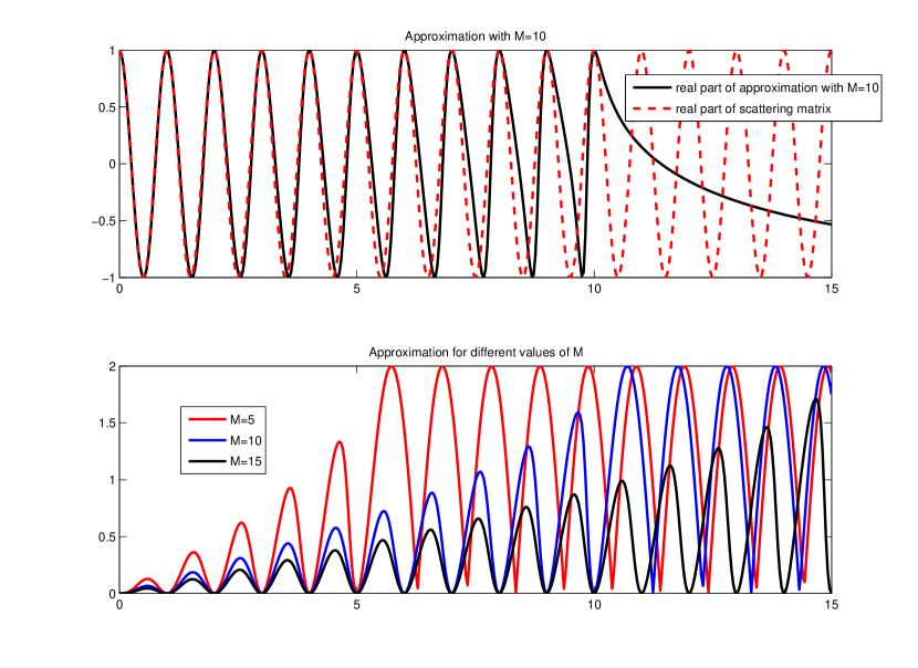
Figure 2. An illustration of the example in §6: the top figure shows the real parts of the approximation and of the scattering matrix, and the lower one, the graphs of $|S_{M^{2}}(k)-S(k)|$ for different values of $M$.

Let $X=(-\pi,\infty)$, with $X_{0}=(-\pi,0]$ and $X_{1}=[0,\infty)$. We consider the operator $-\partial^{2}_{x}$ on $X$, with Neumann boundary conditions. Although strictly speaking this example does not fall in the class considered in the first part of the note ($\overline{X}$ has a boundary, $\{-\pi\}$), it is easy to see the arguments of the previous sections follow through, with $\partial X_{0}$ replaced by $Y=\{0\}$. Because $Y$ is a point, the full scattering matrix is a scalar, and is easily computed to be $S(k)=e^{2\pi ik}$.

For this example,

$$\Psi_{n}(x)=\left\{\begin{array}[]{ll}\pi^{-1/2}&\;\text{if $n=0$}\\ (2/\pi)^{1/2}\cos(nx)&\text{\ if $n>0$}.\end{array}\right.$$

Since there is no sense in the cutoff $\Pi^{\partial X_{0}}_{\Lambda}$ for this problem, we use only one subscript on our approximations of $W$:

$$W_{M^{2}}(k)\stackrel{{\scriptstyle\rm{def}}}{{=}}\sqrt{k}\sum_{n=0}^{M}\Psi_{n}(0)\Psi_{n}(x).$$

Similarly, we denote the approximation of $S(k)$ thus obtained by $S_{M^{2}}(k)$. In the notation of the paper $M=\sqrt{N}$. We denote by $\widetilde{W}_{M^{2}}=\widetilde{W}_{M^{2}}(k)$ the $M+1$ vector $\pi^{-1/2}(1,\sqrt{2},...,\sqrt{2})^{t}$.

Note that if $ia^{t}a\not=-1$,

$$(I+iaa^{t})^{-1}=I-i(1+ia^{t}a)^{-1}aa^{t}.$$

Set $D_{M^{2}}=D_{M^{2}}(k)$ to be the $M+1\times M+1$ matrix given by $((k^{2}-n^{2})\delta_{nm})$. We see that when $k\not\in{\mathbb{Z}}$ so that $D_{M^{2}}(k)$ is invertible, the approximation $S_{M^{2}}(k)$ is given by

$$S_{M^{2}}(k) =-1+2i\widetilde{W}_{M^{2}}^{t}(D_{M^{2}}+i\widetilde{W}_{M^{2}}\widetilde{W}_{M^{2}}^{t})^{-1}\widetilde{W}_{M^{2}}$$

$$=-1+2i(D_{M^{2}}^{-1/2}\widetilde{W}_{M^{2}})^{t}(I+iD^{-1/2}_{M^{2}}\widetilde{W}_{M^{2}}(D^{-1/2}_{M^{2}}\widetilde{W}_{M^{2}})^{t})^{-1}D_{M^{2}}^{-1/2}\widetilde{W}_{M^{2}}.$$

Set $B_{M^{2}}=D_{M^{2}}^{-1/2}\widetilde{W}_{M^{2}}$ and $\beta_{M^{2}}=B_{M^{2}}^{t}B_{M^{2}}$. Then, for $k\not\in{\mathbb{Z}}$,

$$S_{M^{2}}(k) =-1+2iB_{M^{2}}^{t}(I-i(1+i\beta_{M^{2}})^{-1}B_{M^{2}}B_{M^{2}}^{t})B_{M^{2}}$$

(6.1) $$=-1+2i\left(\beta_{M^{2}}-i\frac{\beta_{M^{2}}^{2}}{1+i\beta_{M^{2}}}\right).$$

Now

(6.2) $$\beta_{M^{2}}=\frac{1}{\pi}\left(\frac{1}{k}+\sum_{n=1}^{M}\frac{2k}{k^{2}-n^{2}}\right).$$

We note that

$$\lim_{M\rightarrow\infty}\beta_{M^{2}}=\cot\pi k;$$

one can use this and (6) to see that

$$\lim_{M\rightarrow\infty}S_{M^{2}}(k)=e^{2\pi ik}=S(k)$$

when $k^{2}\not\in{\mathbb{N}}_{0}$. Using (6) and (6.2), we see that for $k\in{\mathbb{R}}\setminus{\mathbb{Z}}$ and $M>|k|$,

$$C_{1}/M\leq|S_{M^{2}}(k)-S(k)|\leq C_{2}/M$$

for some positive constants $C_{1}$, $C_{2}$ depending on $k$. Since $M=\sqrt{N}$, this shows that the estimates obtained in Lemma 4.5 and in the main theorem are optimal.

References

- [1] G. Akguc and L.E. Reichl, Effect of evanescent modes and chaos on deterministic scattering in electron waveguides, Phys. Review E 64(2001), 056221.
- [2] T. Christiansen, Scattering theory for manifolds with asymptotically cylindrical ends. J. Funct. Anal. 131 (1995), 499–530.
- [3] S. Datta, Electronic Trasnport in Mesoscopic Systems, Cambridge Univ. Press, 1995.
-
[4]
L.C. Evans and M. Zworski, Lectures on Semiclassical Analysis
http://math.berkeley.edu/zworski/semiclassical.pdf - [5] D.S. Fisher and P.A. Lee, Relation between conductivity and transmission matrix, Phys. Rev. B 23(1981), 6851–6854.
- [6] T. Guhr, A. Müller-Groeling, and H.A. Weidenmuller, Random Matrix Theories in Quantum Physics:n Common Concepts. Physics Reports 299: 189-428 (1998).
- [7] L. Hörmander, The Analysis of Linear Partial Differential Operators, Vol.III, Springer-Verlag, Berlin, 1985.
- [8] T. Kato, Perturbation theory for linear operators. Second edition, Springer-Verlag, Berlin-New York, 1976
- [9] C. Mahaux and H.A. Weidenmüller, Comparison between the R-Matrix and Eigenchannel Methods, Phys. Rev. 170(1968), 847–856.
- [10] R.B. Melrose, The Atiyah-Patodi-Singer Index Theorem, A K Peters, Wellesley, 1993.
- [11] K. Pichugin, H. Schanz, and P. Šeba, Effective coupling for open billiards, Physical Review E 64 (2001), 056227-1–056227-7.
- [12] D.V. Savin, V.V. Sokolov, and H-J. Sommers, Is the concept of the non-Hermitian effective Hamiltonian relevant in the case of potential scattering? Phys. Rev. E 67, 026215 (2003).
- [13] J. Sjöstrand and M. Zworski, Elementary linear algebra for advanced spectral problems, Annales de l’Institut Fourier, 57(2007), 2095–2141.
- [14] H.-J. Stöckmann, E. Persson, Y.-H. Kim, M. Barth, U. Kuhl, and I. Rotter, Effective Hamiltonian for a microwave billiard with attached waveguide, Phys. Rev. E 65(2002), 066211.