The Footprint of F-theory at the LHC

Abstract

Recent work has shown that compactifications of F-theory provide a potentially attractive phenomenological scenario. The low energy characteristics of F-theory GUTs consist of a deformation away from a minimal gauge mediation scenario with a high messenger scale. The soft scalar masses of the theory are all shifted by a stringy effect which survives to low energies. This effect can range from $0$ GeV up to $\sim 500$ GeV. In this paper we study potential collider signatures of F-theory GUTs, focussing in particular on ways to distinguish this class of models from other theories with an MSSM spectrum. To accomplish this, we have adapted the general footprint method developed recently for distinguishing broad classes of string vacua to the specific case of F-theory GUTs. We show that with only $5$ fb^-1 of simulated LHC data, it is possible to distinguish many mSUGRA models and low messenger scale gauge mediation models from F-theory GUTs. Moreover, we find that at $5$ fb^-1, the stringy deformation away from minimal gauge mediation produces observable consequences which can also be detected to a level of order $\sim\pm 80$ GeV. In this way, it is possible to distinguish between models with a large and small stringy deformation. At $50$ fb^-1, this improves to $\sim\pm 10$ GeV.

1 Introduction

Bridging the gap between string theory and experiment would at first appear to require enormous energy scales to probe more intrinsically “stringy phenomena”. This is compounded by the fact that a given low energy theory may possess several completions at higher energy scales. Indeed, at low energy scales string theory can always be represented by an effective field theory.

On the other hand, there is no guarantee that a given effective field theory will have a UV completion in string theory. Thus, while a direct confirmation of the theory may not be possible, indirect manifestations of the theory are likely to be present at lower energy scales. In particular, although a given string compactification may reduce to a well-defined effective field theory, the specific choice of the field content, mass scales and parameters will very much depend on the details of the compactification. Seemingly contrived field theories may have a very natural stringy origin. In this way, a class of string theory compactifications can provide a preferred set of effective field theories, each with a specific class of potential observable signatures.

From the perspective of the string theorist, the primary challenge is then to determine a set of criteria which select a class of UV completions of the Standard Model of particle physics. One well-motivated possibility is to assume the existence of low scale supersymmetry with the spectrum of the MSSM, and the presence of a Grand Unified Theory (GUT) at high energy scales $M_{GUT}\sim 10^{16}$ GeV. This has typically been taken as evidence for the existence of an extra unification structure near the Planck scale, which is indeed very suggestive of the potential relevance of stringy physics. Thus, in an indirect way, the requirement of GUT scale physics and the existence of supersymmetry manifested at low scales provides a first criterion for vacuum selection.

Although the GUT scale is very close to the Planck scale, there is still a small hierarchy in that $M_{GUT}/M_{pl}\sim 10^{-3}$. In [1] it was proposed that the smallness of this parameter be promoted to the additional selection criterion that a candidate vacuum should admit a limit where the dynamics of quantum gravity can in principle decouple (as $M_{pl}\rightarrow\infty$). A surprising consequence of the existence of both a GUT and a decoupling limit is that it imposes strong restrictions on the content of the low energy theory. In the particular context of compactifications of a strongly coupled formulation of type IIB string theory known as F-theory, this question has been studied. See [2, 1, 3, 4, 5, 6, 7, 8, 9, 10, 11, 12, 13, 14, 15, 16, 17, 18, 19, 20] for recent work on F-theory based models of Grand Unified Theories (F-theory GUTs). Returning to the form of the low energy theory, bottom up considerations also serve to constrain the details of the compactification. Proceeding iteratively, it was shown in [4, 5] that the sparticle spectrum is constrained to a remarkable degree.

From the perspective of the low energy theory, there are two novel features associated with the supersymmetry breaking sector of F-theory GUTs. First, because there exists a limit where gravity decouples, F-theory GUTs are incompatible with gravity mediated supersymmetry breaking, but rather, most naturally accommodate gauge mediated supersymmetry breaking (GMSB). F-theory GUTs constitute a deformation away from the minimal GMSB scenario both in terms of the most natural input energy scales, and in the form of additional contributions to the soft mass terms of the theory.

Recall that in minimal GMSB, the effects of supersymmetry breaking are parameterized by the number of vector-like pairs of messengers in the $5\oplus\overline{5}$, $N_{5}$, and the characteristic mass scale for gauginos, $\Lambda$, such that the mass of the gaugino at a low energy scale is:

$$m_{\text{gaugino}}\sim N_{5}\frac{\alpha}{4\pi}\Lambda\sim N_{5}\frac{\alpha}{4\pi}\frac{F}{M_{\text{mess}}}\text{,}$$ (1)

where $\alpha$ is shorthand for the fine structure constants of the various Standard Model gauge groups, $\sqrt{F}$ is the scale of supersymmetry breaking, and $M_{\text{mess}}$ is the mass of the messenger fields communicating supersymmetry breaking to our sector. From the low energy point of view, it is most natural to take the messenger scale as low as possible without running into conflict with experiments so that $\sqrt{F}\sim M_{\text{mess}}\sim 10^{5}$ GeV. By contrast, in F-theory GUTs the scale of supersymmetry breaking is typically much higher, and is given by $\sqrt{F}\sim 10^{8}-10^{9}$ GeV, and the messenger scale is $M_{\text{mess}}\sim 10^{12}$ GeV. Even though such high values are allowed from the viewpoint of mGMSB, there is nothing distinguished about such energy scales based on low energy considerations. Rather, the requirement that this model admit a UV completion within F-theory requires an increase in the scale of supersymmetry breaking. This is because the $\mu$ term is generated by GUT scale dynamics so that only a small range of scales for supersymmetry breaking will generate a value for the $\mu$ parameter near the scale of electroweak symmetry breaking [4].

Besides motivating a specific high energy scale for the masses of the messenger fields, there are also more stringy manifestations of F-theory GUTs which survive to low energies. These effects constitute a predictive and measurable shift away from the soft supersymmetry breaking terms of the minimal gauge mediation scenario. This deformation is due to the fact that in any quantum theory of gravity, global symmetries must be gauged, or will be violated by Planck scale effects. One such gauge symmetry which is broken at the string scale persists as a global $U(1)_{PQ}$ Peccei-Quinn symmetry at lower energies. In the low energy theory, this global $U(1)$ symmetry is anomalous and so would seemingly lead to an inconsistent theory if gauged. In string theory, however, such anomalies are cancelled via the generalized Green-Schwarz mechanism. What is particularly interesting is that because the fields of the MSSM and supersymmetry breaking sector are both charged under this symmetry, heavy $U(1)_{PQ}$ gauge boson exchange generates additional contributions to the soft scalar masses. Because the charges of all of the MSSM fields are constrained by the existence of higher GUT symmetries, this amounts to a predictive, and stringy prediction for the expected shifts in the mass spectrum away from the minimal gauge mediation scenario. Typically, the size of these mass shifts are comparable to the total mass of the sleptons generated by gauge mediation effects. Therefore this stringy “PQ deformation” will have measurable consequences.

The aim of the present paper is to study collider signatures of F-theory GUTs, and in particular, to establish whether it is possible to distinguish between other models with an MSSM spectrum, but with different input Lagrangians at the TeV scale. In this regard, our goal is to view the LHC as a tool by which one can differentiate between distinct extensions of the Standard Model.

One particularly promising way to distinguish between distinct models with only limited integrated luminosity is based on the general footprint method developed in [21, 22]. This consists of creating two-dimensional plots of various candidate signatures and scanning over the parameters in a given class of models. Performing such a scan for two classes of models, it is then possible to determine a set of signatures which can distinguish between distinct models. This can then be supplemented by more quantitative measures such as chi-square like fits to establish the distinguishability of two models. To minimize the effects of Standard Model background, we have typically selected events which contain either a hard jet, or some other hard process which is difficult to replicate by purely Standard Model effects.

In this paper, we show that with $5$ fb^-1 of simulated LHC data (which is lower than the expected annual luminosity for the LHC in the first three years), it is possible to distinguish F-theory GUTs from other models with an MSSM sparticle spectrum. In F-theory GUTs, the bino or the lightest stau typically corresponds to a quasi-stable NLSP which decays outside the detector. Because reconstruction of the charged track left by a stau is a relatively easy signature to detect, in this paper we will primarily focus on the case of a bino NLSP. Within this class of F-theory GUT models, we scan over the various parameters of the theory, and compare the signals obtained with those of mSUGRA models with mass spectra similar to those of F-theory GUTs. Scanning over many such mSUGRA models, we show that there are indeed signatures which can reliably distinguish between F-theory GUTs and such models. In a certain sense, this is to be expected, because when the squark (resp. slepton) mass spectra are similar to those of F-theory GUTs, the slepton (resp. squark) masses are typically different. Moreover, in those cases where both the squark and slepton spectra are similar, the corresponding branching fractions between the two classes of models are different enough that it is still possible to develop a class of signatures which can distinguish between F-theory GUTs and mSUGRA models. We also find that is possible to distinguish F-theory GUTs from minimal gauge mediation scenarios with a low messenger scale.

At the next stage of analysis, we show that with the same integrated luminosity, it is possible to distinguish between high scale minimal gauge mediation models, and F-theory GUTs. This amounts to showing that the effects of the F-theoretic PQ-deformation are observable at the LHC. To this end, we first show that it is possible to determine a class of signatures which are sensitive to $N_{5}$ and $\Lambda$. Having fixed these values, we next show that in the case of single messenger models, it is indeed possible to roughly distinguish between models with distinct values of the PQ deformation up to a level of $\sim\pm 80$ GeV with $5$ fb^-1 of integrated luminosity. We find that this sensitivity improves to an uncertainty of $\sim\pm 10$ GeV with $50$ fb^-1 of simulated LHC data. In the case of multiple messenger models, the effects of the PQ deformation are less pronounced in the regime where the bino is the NLSP. As a consequence, distinguishing between models in this range of models appears more challenging.

The organization of the rest of this paper is as follows. In section 2 we provide additional background on F-theory GUTs. This includes a more detailed description of the parameter space of F-theory GUTs, and the defining characteristics of F-theory GUTs which are relevant for collider studies. This is followed in section 3 by an analysis of signatures which can distinguish between F-theory GUTs, mSUGRA models, and low messenger scale minimal gauge mediation models. Next, in section 4 we study the extent to which it is possible to distinguish between distinct F-theory GUTs. Section 5 contains our conclusions.

2 F-theory at the LHC

In this section we define the class of models which correspond to F-theory GUTs, and in particular, the low energy content of relevance for collider studies. We refer the interested reader to [4, 5] for further details on the reasoning by which a narrow and predictive range of parameters is determined. For further details of F-theory GUTs, we refer the interested reader to [2, 1, 3, 4, 5, 6, 7, 8, 9, 10, 11, 12, 13, 14, 15, 16, 17, 18, 19, 20].

At low energies, an F-theory GUT corresponds to a deformation away from a minimal gauge mediation scenario. The relatively high messenger scale required to generate a viable $\mu$ term implies that in this class of models, the LSP is the gravitino with a mass of $\sim 10-100$ MeV, and the NLSP is either a quasi-stable bino-like lightest neutralino, or a quasi-stable stau. In scenarios with a stau NLSP the decay of $\widetilde{\chi}_{1}^{0}\rightarrow\widetilde{\tau}_{1}^{\pm}\tau^{\mp}$ will produce staus which will leave a charged track which is relatively easy to detect. In the similar “sweet spot” model of gauge mediation with a high messenger scale, an analysis of a quasi-stable stau NLSP scenario was recently considered [23]. See for example, references [24, 25, 26, 27] for additional information on collider studies of quasi-stable stau NLSP scenarios. Indeed, if this parameter range for F-theory GUTs is realized in nature, it will show up as a striking signal at the LHC, the essential point being that because the stau leaves a charged track, it is then possible to reconstruct the mass of the stau and then the associated decay products. Proceeding up the decay chain, it is then possible to reconstruct more detailed information regarding the mass spectrum of such a scenario. Due to the fact that this analysis has already been performed, e.g. in [27, 23], and is itself based on earlier analysis of quasi-stable stau NLSP scenarios, in this paper we shall focus on the more challenging case of F-theory GUTs with a bino NLSP.

The remainder of this section is organized as follows. After reviewing the main features of the low energy theory, we next describe the scan over parameter space of F-theory GUT models. This is followed by a discussion of the characteristic features of the mass spectrum, cross sections, and branching fractions, and in particular, the dependence of these quantities on the inputs of F-theory GUTs.

2.1 Review of F-theory GUTs

In F-theory GUTs, the defining features of the GUT model are determined by the worldvolume theory of a seven-brane which fills our spacetime and wraps four internal directions of the six hidden dimensions of string theory. The chiral matter of the MSSM localizes on Riemann surfaces in the seven-brane, and interaction terms between chiral matter localize at points in the geometry. As argued in [4], crude considerations based on the existence of a limit where the effects of gravity can decouple imposes sharp restrictions on the low energy content of the effective field theory. In particular, because such models admit a limit where the effects of gravity can decouple, they are incompatible with mechanisms such as gravity mediation. Rather, in F-theory GUTs the effects of supersymmetry breaking are communicated to the MSSM via gauge mediation.

From the perspective of the low energy effective theory, the defining characteristic of F-theory GUTs is that it constitutes a deformation away from a high scale minimal gauge mediation scenario. Letting $X$ denote the GUT singlet chiral superfield which develops a supersymmetry breaking vev:

$$\left\langle X\right\rangle=x+\theta^{2}F_{X}\text{,}$$ (2)

the characteristic mass scales associated with the sparticle spectrum in minimal gauge mediation are controlled by the parameter:

$$\Lambda=\frac{F_{X}}{x}\text{.}$$ (3)

For example, in a model with $N_{5}$ vector-like pairs of messenger fields in the $5\oplus\overline{5}$ of $SU(5)$, the masses of the gauginos and scalar sparticles scale as:

$$m_{\text{gaugino}} \sim N_{5}\frac{\alpha}{4\pi}\Lambda$$ (4)

$$m_{\text{scalar}} \sim\sqrt{N_{5}}\frac{\alpha}{4\pi}\Lambda$$ (5)

where in the above, $\alpha$ is shorthand for the contribution from the various fine structure constants of the Standard Model gauge groups.

In the specific context of F-theory GUTs, the $\mu$ term is roughly given as:

$$\mu\sim\frac{F_{X}}{M_{X}^{KK}}\text{,}$$ (6)

where $M_{X}^{KK}\sim 10^{15}$ GeV is a Kaluza-Klein mass scale of a GUT singlet in the compactification. Thus, obtaining the correct value of $\mu$ requires:

$$F_{X}\sim 10^{16}-10^{18}\text{ GeV}^{2}\text{.}$$ (7)

This range of values for $F_{X}$ implies that the mass of the gravitino is $\sim 10-100$ MeV. Moreover, the fact that the scale of supersymmetry breaking is relatively high compared to other models of gauge mediation implies that the NLSP will decay outside the detector due to its long lifetime.

The rough range of values for $\Lambda$ extends from $\Lambda\sim 10^{4}$ to $\Lambda\sim 10^{6}$. Beyond this range, the mini-hierarchy problem is exacerbated. In fact, we shall typically consider a smaller range on the order of:

$$10^{4}\text{ GeV}\lesssim\Lambda\lesssim 2\times 10^{5}\text{ GeV,}$$ (8)

because for larger values of $\Lambda$, the masses of the gluinos and squarks would be too heavy to be produced at the LHC. Finally, in the context of F-theory GUTs, the $B\mu$ term and the A-terms all vanish at the messenger scale. Thus, in this class of models, $B\mu$ and the A-terms are radiatively generated, and $\tan\beta$ is typically in the range of $20-40$.

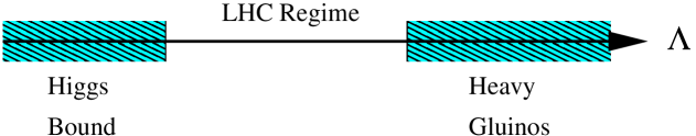
Figure 1: The range of values for the F-theory GUT parameter $\Lambda$ extends from a lower bound set by the current limits on the mass of the Higgs, to an upper bound determined by the requirement that the gluinos be light enough to be produced at the LHC.

The mass spectrum of F-theory GUTs corresponds to a deformation away from the minimal gauge mediation scenario. This is due to the fact that the theory contains an anomalous $U(1)_{PQ}$ gauge symmetry. This anomaly is cancelled via the generalized Green-Schwarz mechanism. The essential point is that this introduces additional higher dimension operators into the theory which have the effect of shifting by a universal amount the soft scalar masses:

$$m_{\text{soft}}^{2}=\widehat{m}^{2}+e_{\Phi}\Delta_{PQ}^{2}\text{,}$$ (9)

where $\widehat{m}$ denotes the mass in the absence of the PQ deformation, and the charge $e_{\Phi}$ is defined as:

Chiral Matter $$\text{: }e_{\Phi}=-1$$ (10)

Higgs $$\text{: }e_{\Phi}=+2\text{.}$$ (11)

To leading order, the gaugino masses and trilinear couplings are unchanged by this deformation.

At a more fundamental level, the deformation parameter originates from integrating out a heavy gauge boson of mass $M_{U(1)_{PQ}}$ so that:

$$\Delta_{PQ}^{2}\sim 4\pi\alpha_{PQ}\frac{F_{X}^{2}}{M_{U(1)_{PQ}}^{2}}\text{,}$$ (12)

where $\alpha_{PQ}$ denotes the fine structure constant of the $U(1)_{PQ}$ gauge theory. A priori, the value of this gauge boson mass can be on the order of the string scale, GUT scale, or even somewhat lower. The phenomenologically most interesting region of course corresponds to the case of lower $M_{U(1)_{PQ}}$, or higher $\Delta_{PQ}$.

In fact, the cosmology of F-theory GUTs suggest a lower bound on $\Delta_{PQ}$ on the order of [7]:

$$\Delta_{PQ}\gtrsim 50\text{ GeV.}$$ (13)

This comes from the fact that in F-theory GUTs, the Goldstone mode associated with $U(1)_{PQ}$ symmetry breaking is the QCD axion [4]. The other real degree of freedom in the associated supermultiplet is the saxion, which has a mass proportional to $\Delta_{PQ}$. As shown in [7], the oscillations of the saxion eventually come to dominate the energy density of the Universe, and its decay reheats the Universe provided the saxion is sufficiently heavy so that a decay channel to a mode other than axions is available. This imposes the kinematic constraint that the saxion be heavier than the Higgs, which translates into the lower bound given by inequality (13).

There is also an upper bound to the size of $\Delta_{PQ}$ because increasing $\Delta_{PQ}$ decreases the soft masses of the squarks and sleptons. Thus, for large enough values of $\Delta_{PQ}$ on the order of $500$ GeV (the precise value of which depends on $\Lambda$ and the number of messenger fields), the low energy spectrum will contain a tachyon. Depending on the number of messengers as well as the size of the PQ deformation, either a bino-like neutralino, or a lightest stau could be the NLSP. Due to the fact that the scale of supersymmetry breaking is so high, the NLSP decays outside the detector, effectively behaving as a stable particle.

Figure 2: The PQ deformation parameter $\Delta_{PQ}$ of F-theory GUTs lowers the squark and slepton soft scalar masses in relation to the value expected from a high messenger scale model of minimal gauge mediated supersymmetry breaking. At $\Delta_{PQ}=0$, F-theory GUTs reduce to a high messenger scale mGMSB model. Cosmological considerations impose a lower bound on $\Delta_{PQ}$ of order $50$ GeV. Finally, there is also an upper bound on $\Delta_{PQ}$ which comes from the requirement that the slepton sector not contain a tachyonic mode.

It is quite exciting that a remnant of stringy physics in the form of the PQ deformation has a measurable manifestation at low energy scales. One of the aims of this paper is to study how the effect of this deformation can be extracted from collider data.

2.2 Parameter Space Scan

Due to the fact that F-theory GUTs depend on one discrete parameter, $N_{5}$, and two continuous parameters, $\Lambda$ and $\Delta_{PQ}$, it is possible to perform a scan over much of the parameter space of models. The range of the scan performed over the parameters $\Lambda$ and $\Delta_{PQ}$ depends on the number of messengers $N_{5}$, because if the masses of the gluinos and squarks are too heavy, the LHC will not be able to generate sparticles of the desired mass. For example, in minimal GMSB, the masses of the gluinos and squarks respectively scale as $N_{5}\Lambda$ and $\sqrt{N_{5}}\Lambda$. Thus, even a factor of five increase in $\Lambda$ can jeapordize the production of gluinos at the LHC. Further, increasing $\Lambda$ exacerbates the fine tuning already present in the Higgs sector. For this reason, we believe it is theoretically well-motivated to primarily consider scenarios where $\Lambda$ is as small as possible, without violating current experimental lower bounds on the masses in the sparticle spectrum. As explained earlier, we will focus on bino NLSP scenarios because the lightest stau NLSP scenario of similar models has been studied elsewhere, such as in [23]. Nevertheless, some distinctive features of such models in the context of F-theory GUTs are discussed briefly in subsection 2.6.

Restricting to the bino NLSP case, since increasing the number of messengers lowers the stau mass relative to the gaugino masses, the condition that the masses satisfy the relation:

$$m_{\widetilde{B}}<m_{\widetilde{\tau_{1}}}$$ (14)

translates into the requirement that:

$$1\leq N_{5}\leq 3\text{.}$$ (15)

Moreover, as $\Lambda$ decreases, the Higgs mass also decreases. Thus, the bound on the Higgs mass obtained from LEP II puts a lower bound on $\Lambda$, which we denote by $\Lambda^{min}(N_{5})$. The maximum value of $\Lambda$ we consider, which we denote by $\Lambda^{max}(N_{5})$ is chosen so that the resulting sparticle masses are light enough to generate enough events at the LHC after a few years. We note that both $\Lambda^{min}(N_{5})$ and $\Lambda^{max}(N_{5})$ are fairly insensitive to $\Delta_{PQ}$. For each scanned value of $\Lambda$, we also scanned over $\Delta_{PQ}$ from $\Delta_{PQ}=0$ to a value of $\Delta_{PQ}$ such that $m_{\widetilde{\tau_{1}}}-m_{\widetilde{B}}<10$ GeV. To summarize, in this paper we have scanned over F-theory GUTs in the parameter range:

• $1\leq N_{5}\leq 3$

• $\Lambda^{min}(N_{5})\leq\Lambda\leq\Lambda^{max}(N_{5})$

• $0\leq{\Delta_{PQ}\leq}\Delta_{PQ}^{max}(N_{5},\Lambda)$.

2.3 Mass Spectrum

Scanning over all regions of interest in F-theory parameter space, we have generated the associated sparticle spectra using SOFTSUSY [28] by imposing the boundary condition $B\mu=0$ at the messenger scale. Compatibility with electroweak symmetry breaking then fixes $\tan\beta$ to a large value between $20-40$, the exact value of which depends on the specifics of the model. The dependence of the mass spectrum on $N_{5}$ and $\Lambda$ when $\Delta_{PQ}=0$ corresponds to the case of mGMSB with a high messenger scale $M_{\text{mess}}\sim 10^{12}$ GeV. See, for example, [29] for a review of gauge mediated supersymmetry breaking. In this section, we discuss the effect of $\Delta_{PQ}$ on the mass spectrum.

The spectrum separates into those particles which are affected by the PQ deformation, and those which are not. To leading order, the masses of the gauginos are not affected by the PQ deformation. Just as in minimal gauge mediation, the low scale gaugino masses $m_{i}$ of the three gauge group factors satisfy the relation:

$$m_{1}:m_{2}:m_{3}\sim 1:2:6\text{.}$$ (16)

In the context of F-theory GUTs, the two lightest neutralinos and the lightest chargino correspond to gauginos, with a primarily bino-like lightest neutralino.

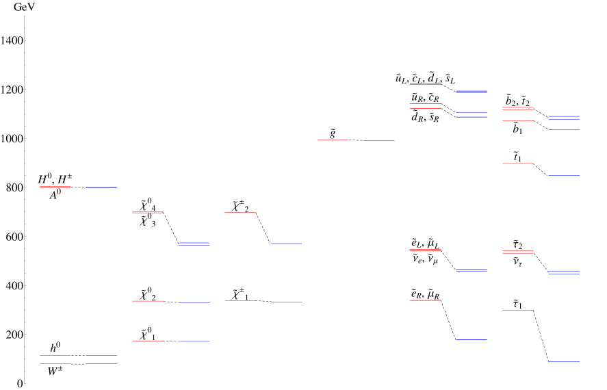
Figure 3: Plot of the mass spectrum of F-theory GUTs with $N_{5}=1$, $\Lambda=1.3\times 10^{5}$ GeV, and minimal (red, left part of each column) and maximal (blue, right part of each column) PQ deformation. See figure 29 in Appendix F for the spectra of three messenger models.

The spectrum of MSSM particles which are not affected by the PQ deformation are therefore:

$$\text{NPQ: }\widetilde{\chi}_{1}^{0}\text{, }\widetilde{\chi}_{2}^{0}\text{, }\widetilde{\chi}_{1}^{\pm}\text{, }\widetilde{g}\text{,}$$ (17)

where we have ordered the sparticles from lightest on the left to heaviest on the right.

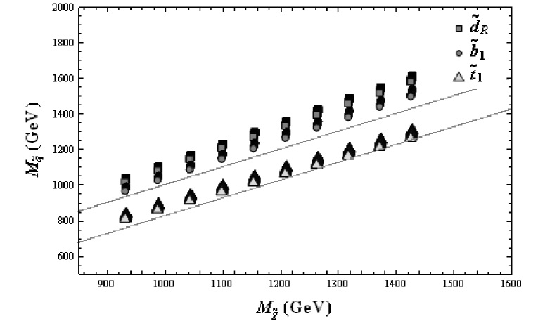
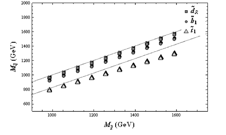
Figure 4: Plots of squark masses versus the gluino mass in F-theory GUTs. The top and bottom plots are for one and two messenger models respectively. The upper line in the plots corresponds to $m_{\tilde{g}}$, while the lower one corresponds to $m_{\tilde{g}}-m_{t}$. These figures imply that the decay of the gluino in one messenger models proceeds via a 3-body process, but in two messenger models it decays in a two-body one. The three messenger case is similar to the two messenger case. The gluino mass is primarily determined by $\Lambda$, and the variations of the squark masses in these figures are due to the change of $\Delta_{PQ}$.

The masses of the remaining sparticles of the MSSM all shift due to the PQ deformation. This includes not just the squarks and sleptons, but also the Higgsinos. This latter shift is more indirect, and can be traced back to the fact that the PQ deformation alters the form of the scalar Higgs potential. As a consequence, achieving proper electroweak symmetry breaking leads to a shift in the value of the $\mu$ parameter at the messenger scale. This in turn alters the masses of the Higgsinos. The spectrum of MSSM particles which are affected by the PQ deformation ordered by lowest mass sparticles on the left to most massive on the right are:

$$\text{PQ: }\widetilde{l}\text{, }\widetilde{\chi}_{3}^{0}\text{, }\widetilde{\chi}_{4}^{0}\text{, }\widetilde{\chi}_{2}^{\pm}\text{, }\widetilde{q}\text{.}$$ (18)

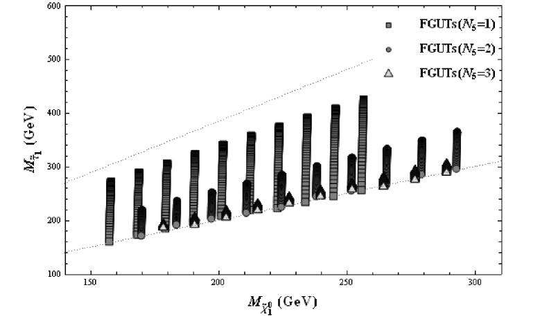
Figure 5: Plot of the stau masses in F-theory GUTs versus the bino NLSP mass for $N_{5}=1,2,3$ messengers. The upper line in the plot corresponds to $m_{\tilde{\chi}_{2}^{0}}$, while the lower one corresponds to $m_{\tilde{\chi}_{1}^{0}}$. This figure shows the typical hierarchy in the masses of $\tilde{\tau}_{1}$ and $\tilde{\chi}_{1,2}^{0}$. The variation in the stau mass corresponds to the change of $\Delta_{PQ}$, which becomes less significant in the bino NLSP regime as the number of messengers increases.

The mass shift due to the PQ deformation is most prominent for lighter sparticles. At the messenger scale, the mass shift for squarks and sleptons is:

$$m=\widehat{m}\sqrt{1-\frac{\Delta_{PQ}^{2}}{\widehat{m}^{2}}}\text{,}$$ (19)

where $\widehat{m}$ denotes the mass at the messenger scale in the absence of the PQ deformation. Hence, when $\widehat{m}\gg\Delta_{PQ}$, there is little change in the mass of the sparticle, so that the squarks will shift by a comparably small amount. On the other hand, the masses of the sleptons can shift significantly. Since the mass spectrum is generated mainly by gauge mediation, the absence of an $SU(2)$ gauge coupling implies that the right-handed selectron $\widetilde{e}_{R}$, smuon $\widetilde{\mu}_{R}$ and stau $\widetilde{\tau}_{R}$ will be lighter, and thus more sensitive to the PQ deformation in comparison with their left-handed counterparts. Depending on the range of parameter space, the $\widetilde{e}_{R}$, $\widetilde{\mu}_{R}$ and $\widetilde{\tau}_{R}$ mass can either be above or below the mass of the $\widetilde{\chi}_{2}^{0}$. It is also possible in some cases for $\widetilde{e}_{R}$, $\widetilde{\mu}_{R}$ and $\widetilde{\tau}_{R}$ to become comparable in mass to $\widetilde{\chi}_{1}^{0}$.

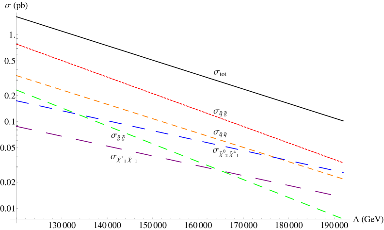
Figure 6: Plot of the cross sections at $14$ TeV CM energy for the primary supersymmetric processes as a function of $\Lambda$ for F-theory GUT models with $N_{5}=1$ and $\Delta_{PQ}=0$ GeV. Note that as $\Lambda$ increases, the cross sections decrease by roughly an order of magnitude. See figure 30 in Appendix F for a similar plot of the $N_{5}=3$ case.

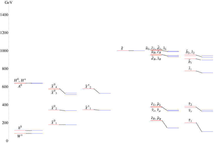
Figure 29: Plot of the mass spectrum of an F-theory GUT with $N_{5}=3$, $\Lambda=4.5\times 10^{4}$ GeV, and minimal (red, left part of each column) and maximal (blue, right part of each column) PQ deformation.

Due to the large Yukawa couplings present in the third generation, RG flow will amplify the effects of the PQ deformation in the third generation squarks and sleptons. The stop and sbottom can typically become lighter than the gluino in such models, and the $\widetilde{\tau}_{1}$ is lighter than $\widetilde{\chi}_{2}^{0}$. A comparison of these mass hierarchies for different number of messengers can be seen in figures 4 and 5. Further, for large enough values of $\Delta_{PQ}$, the $\widetilde{\tau}_{1}$ can be lighter than $\widetilde{\chi}_{1}^{0}$. Figure 3 and figure 29 in Appendix F illustrate the mass spectrum of a single messenger and three messenger model at minimal and maximal PQ deformation. By inspection of these figures, it follows that progressing up in mass tends to diminish the effects of the PQ deformation.

The interplay between $\Delta_{PQ}$ and the mGMSB parameters $N_{5}$ and $\Lambda$ also influences the form of the low energy spectrum. Returning to figures 3 and 29, we note that although it is a well-known aspect of minimal gauge mediation, an important feature of these spectra is that as the number of messengers increases, the scalar sparticles tend to decrease in mass faster than their fermionic counterparts. This will have important consequences when we discuss potential decay chains of interest.

2.4 Cross Sections

We now discuss the dependence of the associated cross sections on the parameters $N_{5}$, $\Lambda$ and $\Delta_{PQ}$. Scanning over F-theory parameter space, we have generated the (leading order) cross sections for parton collisions using PYTHIA [30]. The dominant supersymmetric processes are associated with events where parton collisions generate either two gluinos ($\sigma_{\widetilde{g}\widetilde{g}}$), a squark and a gluino ($\sigma_{\widetilde{q}\widetilde{g}}$), two squarks ($\sigma_{\widetilde{q}\widetilde{q}}$), two lightest charginos ($\sigma_{\widetilde{\chi}_{1}^{+}\widetilde{\chi}_{1}^{-}}$), or a second neutralino and a lightest chargino ($\sigma_{\widetilde{\chi}_{2}^{0}\widetilde{\chi}_{1}^{\pm}}$), where here, $\widetilde{q}$ denotes a first or second generation squark. We have also determined the total cross section generated by all dominant processes, which we denote by $\sigma_{\text{tot}}$.

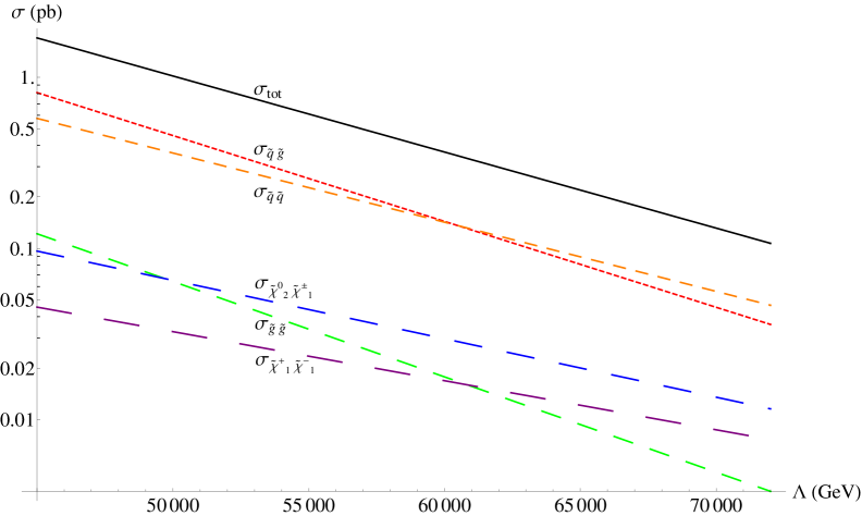
Figure 30: Plot of the cross sections at $14$ TeV CM energy for the primary supersymmetric processes as a function of $\Lambda$ for F-theory GUT models with $N_{5}=3$ and $\Delta_{PQ}=0$ GeV. Note that as $\Lambda$ increases, the cross sections decrease by roughly an order of magnitude.

Figure 6 and figure 30 in Appendix F show plots of the largest cross sections as a function of $\Lambda$ with $\Delta_{PQ}=0$ for $N_{5}=1$ and $N_{5}=3$. Note that as expected, increasing $\Lambda$ tends to decrease the cross section. An interesting feature of these plots is that although they are not colored particles, there is a significant amount of chargino and second neutralino production. In addition, we find that there is only very weak dependence on $\Delta_{PQ}$ in the dominant cross sections. Turning the discussion around, because the cross section has little dependence on $\Delta_{PQ}$, we can deduce that the primary effects from the PQ deformation must originate from shifts in the masses, or branching ratios as a function of $\Delta_{PQ}$.

2.5 Decay Channels

In this subsection we discuss the primary decay channels which are present in F-theory GUTs. Due to the fact that the cross section is dominated by the production of gluinos, squarks, lightest charginos and second lightest neutralinos, these will also be the first particles present in the decay chain. We have computed the relevant branching fractions by linking the output from the mass spectrum calculated via SOFTSUSY [28] with SDECAY [31]. Due to the fact that the relative masses of the squarks and the gluino heavily depends on whether $N_{5}=1$ or $N_{5}>1$, in the following discussion we separate our analysis of these two cases.

2.5.1 Single Messenger Case

First consider single messenger F-theory GUT models. In this case, only the stop and sbottom are typically lighter than the gluino whereas for $N_{5}>1$, all of the squarks are lighter than the gluino. Thus, the gluino decays via off shell squarks to three decay products in the case of $N_{5}=1$ whereas for $N_{5}>1$, two body decays are instead preferred. The dominant decay channels for the gluino at small PQ deformation are presented below in the case of $N_{5}=1$ with $\Lambda=1.44\times 10^{5}$ GeV:

Channel $$\Delta_{PQ}=0$$ GeV

  . (20)

In the above, we have adopted a condensed notation where $\pm$ and $\mp$ refer to the charges of the particle and its anti-particle. Also $q$ refers to the first two quark generations and $q_{1,2}$ refer to distinct components of an $SU(2)$ quark doublet. By inspection, the stringy PQ deformation does produce a change in the branching fractions. Note that the decay of a single $\tilde{g}$ to two tops is a decay which is easy to see with small luminosity [32].

The decay of the right-handed squarks provides another channel which is potentially sensitive to the effects of the PQ deformation. For example, the branching ratios for the decay of the right-handed sdown are:

Channel $$\Delta_{PQ}=0 \Delta_{PQ}=250 \widetilde{d}_{R}\rightarrow\widetilde{\chi}_{1}^{0}d 12\% 15\% \widetilde{d}_{R}\rightarrow\widetilde{g}d 88\% 84\%$$ GeV , (21)

while for the right-handed sup, we find:

Channel $$\Delta_{PQ}=0 \Delta_{PQ}=250 \widetilde{u}_{R}\rightarrow\widetilde{\chi}_{1}^{0}u 31\% 36\% \widetilde{u}_{R}\rightarrow\widetilde{g}u 69\% 64\%$$ GeV . (22)

Similarly for the left-handed sdown and sup, the dominant decay is to gluino plus quark, followed by the decay to chargino plus quark. These decays are all sensitive to the PQ deformation only at the level of a few percent change in the branching fraction.

Next consider the decay of the chargino $\widetilde{\chi}_{1}^{\pm}$ and the second neutralino $\widetilde{\chi}_{2}^{0}$. These channels are especially interesting because their production is not directly accompanied by colored objects. Moreover, in contrast to the other channels considered so far, the branching fractions of $\widetilde{\chi}_{1}^{\pm}$ and $\widetilde{\chi}_{2}^{0}$ both have strong dependence on the PQ deformation. The branching fractions for the decay of $\widetilde{\chi}_{1}^{\pm}$ are:

Channel $$\Delta_{PQ}=0 \Delta_{PQ}=250 \widetilde{\chi}_{1}^{\pm}\rightarrow\widetilde{\tau}_{1}^{\pm}\nu_{\tau} 51\% 85\% \widetilde{\chi}_{1}^{\pm}\rightarrow\widetilde{\chi}_{1}^{0}W^{\pm} 49\% 15\%$$ GeV . (23)

Because increasing the size of the PQ deformation parameter decreases the mass of the stau, more phase space is available for a decay into a stau and tau-neutrino. This large effect may mean it is possible to measure non-zero $\Delta_{PQ}$ by triggering on events with $W^{\pm}$ and $\tau$’s. In certain cases, this is possible because the $\tilde{\chi}_{1}^{\pm}$ production cross section can be $\geq 0.1$ pb.

Next consider the decay of $\widetilde{\chi}_{2}^{0}$. In this case, the relevant branching fractions are:

Channel $$\Delta_{PQ}=0 \Delta_{PQ}=250 \widetilde{\chi}_{2}^{0}\rightarrow\widetilde{\tau}_{1}^{\pm}\tau^{\mp} 51\% 84\% \widetilde{\chi}_{2}^{0}\rightarrow\widetilde{\chi}_{1}^{0}h 43\% 13\% \widetilde{\chi}_{2}^{0}\rightarrow\widetilde{\chi}_{1}^{0}Z 5\% 2\%$$ . (24)

Much as in the decay of $\widetilde{\chi}_{1}^{+}$, the increase in the branching fraction to staus as $\Delta_{PQ}$ increases follows from the fact that as the mass of the stau decreases, more phase space becomes available for a decay into a stau and tau.

2.5.2 Multiple Messenger Case

In contrast to the single messenger case, in the case of multiple messengers, the masses of the scalars are typically lower in comparison to the gauginos. One consequence of this change is that the gluino can now decay to two on-shell products. In addition, the effects of the PQ deformation are typically weaker in the range of values where the bino is the NLSP. This is due to the fact that the stau is already closer in mass to the bino prior to turning on any PQ deformation. For these reasons, we shall focus on decay channels present at zero PQ deformation.

Restricting now to the case of zero PQ deformation, it is of interest to compare multiple messenger models with similar spectra. Letting $\Lambda_{i}$ denote the value of $\Lambda$ in the case of $i$ messengers, we expect a rough degeneracy in the mass spectrum when either the gauginos or scalars have similar masses. A similar gaugino mass spectrum leads to the condition:

$$i\cdot\Lambda_{i}=j\cdot\Lambda_{j}$$ (25)

while a similar scalar mass spectrum requires:

$$\sqrt{i}\cdot\Lambda_{i}=\sqrt{j}\cdot\Lambda_{j}\text{.}$$ (26)

A rough similarity in the mass spectra can therefore be expected in the range of values:

$$\sqrt{\frac{i}{j}}\leq\frac{\Lambda_{i}}{\Lambda_{j}}\leq\frac{i}{j}\text{,}$$ (27)

where without loss of generality, $i\geq j$. As an example, we compare the decay channels for a two and three messenger model such that:

$$\Lambda_{2} =8\times 10^{4}\text{ GeV}$$ (28)

$$\Lambda_{3} =5.7\times 10^{4}\text{ GeV.}$$ (29)

As in the case of the single messenger models, we now determine the primary decay channels for gluinos, right-handed first and second generation squarks, and charginos. The distinction between the various branching fractions then provide a means to extract signals which can distinguish between these cases. In addition, we find that in all cases, there is little shift in the branching fractions at non-zero PQ deformation in the bino NLSP regime.

The dominant decay channel for gluinos is given by decays to squarks. Comparing the two and three messenger models presented above, we find:

Channel $$N_{5}=2 N_{5}=3 \widetilde{g}\rightarrow\widetilde{t}^{\pm}t^{\mp} 82\% 45\% \widetilde{g}\rightarrow\widetilde{b}^{\pm}b^{\mp} 17\% 30\% \widetilde{g}\rightarrow\widetilde{q}_{R}^{\pm}q^{\mp} 0.3\% 25\%$$ . (30)

By inspection, gluinos decay to stops and tops with large branching fractions, thus giving rise to a spectacular four top signature at the LHC [32]. It is interesting to note that similar signature can also arise from the $G_{2}$-MSSM [33]. Further, note that this decay mode is more favored in the two messenger case.

Next consider the decay of the right-handed sdown and sup. We find that in both cases, the dominant decay of the squark is to the lightest neutralino and quark with all other decay channels entirely negligible. This is to be contrasted with the single messenger case, where the dominant decay mode is to a gluino and quark due to the fact that in the single messenger model, the squark is typically heavier than the gluino, whereas in the multiple messenger models, the situation is reversed. The change in the decay of left-handed sdown and sup is similar. Both of these decay dominantly to $\tilde{\chi}_{1}^{\pm}+q^{\prime}$ and $\tilde{\chi}_{2}^{0}+q$. The decay to gluino is now suppressed kinematically.

The decay of $\widetilde{\chi}_{1}^{\pm}$ is roughly similar in the two and three messenger cases, with branching fractions:

Channel $$N_{5}=2 N_{5}=3 \widetilde{\chi}_{1}^{\pm}\rightarrow\widetilde{\tau}_{1}^{\pm}\nu_{\tau} 79\% 82\% \widetilde{\chi}_{1}^{\pm}\rightarrow\widetilde{\chi}_{1}^{0}W^{\pm} 21\% 18\%$$ , (31)

which is again a small effect.

Finally, we also consider decays of $\widetilde{\chi}_{2}^{0}$. The branching fractions are only mildly sensitive to a change in the number of messengers:

Channel $$N_{5}=2 N_{5}=3 \widetilde{\chi}_{2}^{0}\rightarrow\widetilde{\tau}_{1}^{\pm}\tau^{\mp} 78\% 80\% \widetilde{\chi}_{2}^{0}\rightarrow\widetilde{\chi}_{1}^{0}h 19\% 16\% \widetilde{\chi}_{2}^{0}\rightarrow\widetilde{\chi}_{1}^{0}Z 2\% 2\%$$ . (32)

To summarize, we therefore see that the predominant difference between the branching fractions present in the two and three messenger models are dictated by the decays of the gluino. Such signals then provide a means to distinguish between two and three messenger models. Moreover, as indicated earlier, in the regime of parameters where the bino is the NLSP, the PQ deformation in the multiple messenger cases does not lead to a significant change in the sparticle mass spectrum. Therefore, it is expected to be more difficult to distinguish them from mGMSB models.

2.6 F-theory GUTs with a Stau NLSP

While the primary focus of this paper is F-theory GUT scenarios with a bino NLSP, the stau NLSP scenario is also a viable option, and is especially likely for F-theory GUTs with multiple messenger fields. In this subsection we briefly sketch some features of the expected signals in this case, and discuss how to distinguish such models from high messenger scale mGMSB models with a quasi-stable stau NLSP.

When the lightest stau is the NLSP of an F-theory model, it will either leave a highly ionizing track in the tracking chamber or “fake muons ” in the muon chamber of a detector at the LHC. The mass of the lightest stau can be determined by the energy-loss ($dE/dt$) and Time-of-Flight measurement. The other particles further up the decay chain can be constructed as well in principle [27].  For example, by determining the invariant mass resulting from the on shell decays $\widetilde{\chi}_{1,2}^{(0)}\rightarrow\tau^{\pm}\widetilde{\tau}_{1}^{\mp}$, it should then be possible to reconstruct the mass of $\widetilde{\chi}_{1,2}^{0}$.  Kinematic considerations require $m_{\widetilde{\chi}_{1,2}^{0}}>m_{\widetilde{\tau}_{1}}$. In addition, the decay of a first or second-generation right-handed squark via the process $\widetilde{q}_{R}\rightarrow\widetilde{\chi}_{1}^{0}q\rightarrow\widetilde{\tau}_{1}^{\pm}\tau^{\mp}q$ can also be used to extract detailed properties of the spectrum. For example, by observing the trajectory of the lightest stau, it is then possible to reconstruct the four-momentum of $\widetilde{\chi}_{1}^{0}$. Thus, once the mass of $\widetilde{\chi}_{1}^{0}$ has been extracted, the corresponding squark mass can also be specified. While a completely accurate reconstruction may require about $10-30$  fb^-1 of integrated luminosity, this can in principle be accomplished with data from the first three years of the LHC, and therefore provides one reliable method for determining detailed features of the spectrum. In addition to this type of direct mass reconstruction, many of the methods based on a footprint analysis will carry over to the stau NLSP case as well.

Once the masses of the $\widetilde{\tau}_{1}$, $\widetilde{\chi}_{1,2}^{0}$ and $\widetilde{q}_{R}$ have been determined, it will be possible to compare these values with the spectrum expected from mGMSB  with a high messenger scale. Since the masses of the sparticles in mGMSB are determined by $N_{5}$, $\Lambda$ and to a far weaker extent $M_{\text{mess}}$, the masses of the remaining sparticles are fixed by the values of $m_{\text{bino}}$ (or $m_{\text{wino}}$) and $m_{\widetilde{q}_{R}}$. In particular, it is possible to then determine the mass of the lightest stau in a minimal GMSB scenario. Assuming that this determination has been performed, measuring the mass of the lightest stau will then provide a direct way to distinguish between the mGMSB prediction, and the F-theory prediction with non-zero PQ deformation.

3 Distinguishing F-theory GUTs From Other Models

One of the primary aims of this paper is to determine whether the LHC will be able to distinguish F-theory GUTs from other potential extensions of the Standard Model. At the first level of analysis, it is important to establish whether the signatures from the LHC are compatible with the MSSM. This is a topic which has been discussed extensively in the literature, for some recent studies of this kind see [34, 35, 36, 37, 38] and references therein. We shall therefore assume that evidence compatible with the MSSM has been found.

At the next stage of analysis, we would like to establish whether F-theory GUTs can be distinguished from other models with an MSSM spectrum such as mSUGRA, as well as mGMSB scenarios with a low messenger scale. Once we have ruled out these possibilities as potential candidates which can mimic the effects of F-theory GUTs, it is then important to establish that F-theory GUTs can be distinguished from high messenger scale mGMSB scenarios. Because of the similarities between F-theory GUTs and high scale gauge mediation scenarios, we shall postpone this analysis to section 4.

The extent to which we can distinguish a given class of models depends on the integrated luminosity of LHC data. For the most part, we shall simulate $5$ fb^-1 of integrated luminosity. Interestingly, we find that even with just $5$ fb^-1 of simulated LHC data, it is possible to distinguish F-theory GUTs from small A-term mSUGRA models. The primary limitation in this determination is that the squark and gluino masses must be light enough to be produced by the LHC. We also find that it is possible to distinguish large A-term mSUGRA models from single messenger F-theory GUTs. On the other hand, large A-term mSUGRA models can more effectively mimic some of the signatures of multiple messenger F-theory GUTs. Finally, we also show that F-theory GUTs can be distinguished from minimal gauge mediation models with a lower messenger scale.

To perform this analysis, we have adapted the general footprint method of [21, 22] to the case of F-theory GUTs. This consists of developing a set of signatures which will allow us to distinguish between an F-theory GUT and other models, such as mSUGRA models, or even between distinct F-theory GUT models. Given a model, one would like to determine a set of $N$ signatures (the exact value of $N$ depending on the details of the footprint) which are likely to be sensitive to the input parameters of the model. Thus a single model generates an $N$-dimensional vector. The proximity or lack thereof between the vectors of two such theories can then be used to distinguish between different models.

The methodology of the footprint is very general, and consists of scanning over various signatures in a class of models and varying the allowed parameters within a given class. Comparing with other classes of models it is then possible to single out the signatures which are most effective in distinguishing them. These signatures can in principle consist of just counting events, or some combination of counting events with more refined observables. In the footprint method only actual measurable signatures are used, not quantities difficult to measure such as sparticle masses, soft-breaking parameters, or $\tan\beta$. Further, parameters not explicitly fixed by prior considerations are scanned. In this way, we can avoid deriving misleading conclusions based on specific features of a single model or simulation.

Once we have isolated a class of signals which can potentially serve to distinguish an F-theory GUT from other models, the next step is to determine whether at a more quantitative level it is possible to distinguish various models. To this end, we introduce a chi-square like measure of distinguishability, and show that with respect to this measure, it is indeed possible to distinguish between many models.

The rest of this section is organized as follows. We first describe the simulation of signals and Standard Model background. After this, we define in more precise terms the class of mSUGRA models and low scale mGMSB models which we shall compare to F-theory GUTs, paying special attention to signatures which can potentially be used to distinguish F-theory GUTs from these models. After introducing a more quantitative notion of distinguishability in both theory and signature space, we develop a set of signatures which comprise our footprint. Using this set of signatures, we show that in most cases, it is possible to distinguish between F-theory GUTs and mSUGRA models, as well as low messenger scale mGMSB models. We defer a full comparison of F-theory GUTs to high messenger scale mGMSB models to section 4.

3.1 Simulation of Signals and Background

Before proceeding to potential signals of interest, we first describe our simulation of LHC signatures. To simulate the signals of F-theory based models, we use the spectrum and decay table obtained (in SLHA format) by linking SOFTSUSY and SDECAY to generate events using PYTHIA 6.4. These events are then passed to PGS4 [39] for detector simulation. To reduce the number of background events, we have used the PGS trigger with high thresholds, the details of which can be found in Appendix D. In principle, one should include the next-to-leading order correction to the tree-level cross sections used in the PYTHIA. However, since our main purpose is to compare different classes of models, it is not particularly important to include such corrections. In addition, although PGS is a simplified detector simulator and is not tuned to match either ATLAS or CMS, it is still useful as a way to obtain characteristic LHC signatures.

We have simulated $5$ fb^-1 of Standard Model background by including the most important channels $t\overline{t}$, $W/Z$ + jets and $WW/WZ/ZZ$ + jets. In many cases, a significant reduction in QCD background can be achieved by means of sophisticated event selection cuts, which we shall therefore typically neglect. These events are generated using the PYTHIA-PGS package in the same way as the signals. Of course, even though the use of parton-shower Monte Carlo to estimate multi-jet backgrounds is known to underestimate the backgrounds, for our present purposes where $S\gg\sqrt{B}$, it suffices to include just the effects of the PYTHIA simulation.

To obtain LHC signatures, we selected subsets of events with different final state objects: jets, leptons, missing energy. Before the event selection, we impose the following object-level cut:

• photon, lepton, tau: $P_{T}>10$ GeV and $\eta<2.5$

• jets: $\eta<3.0$

Here no jet $P_{T}$ cut is imposed until the event selection.

In order to reduce SM background, we first consider two typical SUSY search channels based on inclusive two jets plus $\displaystyle{\not}E_{T}$, and inclusive four jets plus $\displaystyle{\not}E_{T}$, with selection cuts given in table 1. Both channels are well studied in ATLAS [40] and CMS [41], and the background (mainly from $t\bar{t}$ and W/Z + jets) is known to be controllable in the large effective mass region.

Selection	$2$ jets + $\displaystyle{\not}E_{T}$	$4$ jets + $\displaystyle{\not}E_{T}$
$P_{T}$ (GeV)	$>150$, $100$	$>100$, $50$, $50$, $50$
$\displaystyle{\not}E_{T}$ (GeV)	$>150$	$>100$
$S_{T}$	$>0.2$	$>0.2$
$M_{eff}$ (GeV)	$>1200$	$>1200$

Table 1: Inclusive SUSY search channel selection cuts used in order to reduce SM background.

Here, the Effective Mass $M_{eff}$ is defined as the sum of $P_{T}$ of all objects in an event including the missing energy:

$$M_{eff}\equiv\sum_{i=all}P_{T}^{i}+\displaystyle{\not}E_{T}\text{.}$$ (33)

In addition, $0<S_{T}<1$ denotes the transverse sphericity:

$$S_{T}=\frac{2\lambda_{\text{large}}}{\lambda_{\text{small}}+\lambda_{\text{large}}}$$ (34)

where $\lambda_{\text{large}}$ and $\lambda_{\text{small}}$ denote the large and small eigenvalues of the $2\times 2$ transverse sphericity tensor:

$$\mathbf{S=}\left(\begin{array}[]{cc}\Sigma p_{x}^{2}&\Sigma p_{x}p_{y}\\ \Sigma p_{x}p_{y}&\Sigma p_{y}^{2}\end{array}\right)\text{.}$$ (35)

In the case of SUSY events, the transverse sphericity is typically closer to $S_{T}=1$, indicating a more isotropic event.

From these two inclusive selections, we further divide the events according to the number of leptons, taus and b-jets in the final states. Other signatures include multijets plus $\displaystyle{\not}E_{T}$ with hard jet $P_{T}$ thresholds, and inclusive one tau signatures with various different $P_{T}$ thresholds. For completeness, we also include the signatures which have been found to be effective for testing gaugino mass unification in [42]. In total, we have studied $103$ signatures, which are listed in Appendix C.

Although we have included a large number of candidate signatures, we will see later that only a small subset of these are really effective in distinguishing models. See table 2 for the $10$ signatures selected using the footprint analysis. The details of this footprint analysis will be applied later in the context of specific models. These signatures will also be used later to distinguish F-theory GUTs from other candidate models using a chi-square like measure $\Delta S^{2}$ which shall be introduced in subsection 3.4.

	Signature List A
$1$	$0\tau$($P_{T}>40$),$\geq 2$jets($P_{T}>150,100$)
$2$	$\geq 1\tau$($P_{T}>40$),$\geq 2$jets($P_{T}>150,100$)
$3$	$\geq 2\tau$($P_{T}>40$),$\geq 2$jets($P_{T}>150,100$)
$4$	$0b$($P_{T}>50$),$\geq 2$jets($P_{T}>150,100$)
$5$	$\geq 2b$($P_{T}>50$),$\geq 2$jets($P_{T}>150,100$)
$6$	$\geq 6$jets($P_{T}>100,100,20,20,20,20$)
$7$	$\geq 4$jets($P_{T}>250,250,150,150$)
$8$	$0l$($P_{T}>20$),$\leq 4$jets($P_{T}>50$), $\displaystyle{\not}E_{T}>500$
$9$	$0l$($P_{T}>20$),$\geq 5$jets($P_{T}>50$), $0.5<r_{\rm jet}<1.0$
$10$	$\geq 1l$($P_{T}>20$),$\geq 5$jets($P_{T}>50$), $0.05<\displaystyle{\not}E_{T}/M_{eff}<0.35$

Table 2: List of signatures obtained from a footprint analysis which are effective in distinguishing F-theory GUTs from mSUGRA and low scale mGMSB. These signatures will also be used to distinguish models using a chi-square like measure $\Delta S^{2}$, which shall be introduced in subsection 3.4. All the $P_{T}$ and $\displaystyle{\not}E_{T}$ thresholds are in units of GeV. The variable $r_{\rm jet}$ is defined as $r_{\rm jet}\equiv(P_{T}^{\rm jet3}+P_{T}^{\rm jet4})/(P_{T}^{\rm jet1}+P_{T}^{\rm jet2})$, where $P_{T}^{{\rm jet}i}$ is the transverse momentum of the $i$-th hardest jet in the event.

Before comparing signals for different classes of new physics models, it is important to check that the candidate signal $S$ is sufficiently large compared to the SM background $B$ so that $S>5\sqrt{B}$. As reviewed for example in [42], the discovery condition can also be written as a condition on luminosity

$$L>\gamma^{2}\frac{\sigma_{SM}}{\sigma^{2}}$$ (36)

where $\sigma$ and $\sigma_{SM}$ are respectively the cross sections of a specific channel, and the Standard Model background, and $\gamma$ characterizes the number of sigma for a given confidence level, so that for example a five sigma level of confidence corresponds to $\gamma=5$. For a given luminosity, only those channels which could lead to discovery are important, and these are the only ones we shall consider.

To distinguish models, this criterion must be supplemented by the condition that the difference of two signals is also above the Standard Model background. For example, consider a signal $S_{1}$ and $S_{2}$ with corresponding cross sections $\sigma_{1}$ and $\sigma_{2}$ for two models obtained for given luminosity $L$. When $S<B$, the condition for two models to be distinguishable is:

$$|\sigma_{1}L-\sigma_{2}L|>\gamma\sqrt{\sigma_{SM}L}$$ (37)

The minimal luminosity required for distinguishability is then given by:

$$L_{min}^{DT}=\gamma^{2}\frac{\sigma_{SM}}{(\sigma_{1}-\sigma_{2})^{2}}$$ (38)

By inspection, $L_{min}^{DT}$ increases as the difference in signatures decreases, and could be much larger than the discovery limit. Conversely, as the difference in signatures increases, the minimal luminosity required for distinguishability decreases.

3.2 Mimicking F-theory GUTs

In this section we analyze some models with an MSSM spectrum which can potentially mimic the effects of F-theory GUTs. While it is in principle possible to perform a complete scan over all of the soft supersymmetry breaking terms of the MSSM, in practice, this is computationally not feasible. For this reason, we shall focus on some well known examples with similar spectra to those of F-theory GUTs. To this end, we consider mSUGRA models with small and large universal A-terms, and minimal gauge mediation models with low and high messenger scales. We defer a full comparison between high scale mGMSB models and F-theory GUTs to section 4.

Even when the spectra of two models are similar, there will typically be a difference in the branching fractions which can translate into experimental observables. In this section we discuss from a theoretical standpoint signatures which can potentially distinguish between these models and F-theory GUTs. As throughout this paper, we focus on the case of F-theory GUTs with a bino NLSP.

We begin by discussing the case of mSUGRA models. See Appendix A for further details on the scan of mSUGRA models performed. There are two regimes of interest corresponding to mSUGRA models with small universal A-terms, and large universal A-terms. By the “small A-term” regime we shall mean the region in mSUGRA parameter space where the universal A-term is small, and such that the slepton masses are large compared to the electro-weakinos:

$$m_{\tilde{\tau}}\approx m_{\tilde{e},\tilde{\mu}}>m_{\tilde{\chi}_{1,2}^{0}}\text{,}$$ (39)

which roughly mimics the case of F-theory GUTs, although there is some difference in that $m_{\tilde{\tau}}>m_{\tilde{\chi}_{2}^{0}}$. For these mSUGRA models, $\chi_{2}^{0}$ and $\chi_{1}^{\pm}$ will typically decay into an LSP plus a gauge boson or a Higgs boson. This is in contrast to the case in F-theory based models where decay through the lightest stau $\tilde{\tau}_{1}$ is always important, giving $2\;\tau$ plus missing $E_{T}$ or $4\;\tau$ plus missing $E_{T}$ signatures. Therefore, to distinguish this subset of mSUGRA models, one can look for lepton flavor universality, or more explicitly, whether there are more taus than electrons and muons in the events.

Large A-term mSUGRA models can also potentially mimic the spectrum of F-theory GUTs. By the “large A-term” regime we shall mean the region in mSUGRA parameter space where the universal A-term is large, and where the mass of the lightest stau $\tilde{\tau}_{1}$ is suppressed due to either a large Yukawa, or an A-term such that:

$$m_{\tilde{\chi}_{1}^{0}}<m_{\tilde{\tau}_{1}}<m_{\tilde{\chi}_{2}^{0}}\text{.}$$ (40)

This is the same ordering of masses present in F-theory GUTs with a bino NLSP. Therefore, large A-term models can mimic signals based on the decay of $\chi_{2}^{0}$ to an on-shell stau. Further, although the A-terms of F-theory GUTs are zero at the messenger scale, the high messenger scale implies that radiative corrections can still generate contributions to the A-terms of F-theory GUTs at lower energy scales. In fact, as we will see in section 3.6, this subset of mSUGRA models can for low enough luminosity indeed sometimes be difficult to distinguish from the signatures of F-theory based models.

Minimal GMSB scenarios constitute another class of models which could mimic the signatures of F-theory GUTs. Here, there are two qualitative regimes of interest corresponding to models with a high, or low messenger scale. Since we shall consider the case of high messenger scale models in greater detail in section 4, in this section we focus on the comparison between F-theory GUTs and low messenger scale mGMSB models. In contrast to F-theory GUTs where the NLSP always decays outside the detector, in the case of a low scale GMSB model, the NLSP decays inside the detector. In principle, the NLSP can correspond either to a bino-like neutralino, or the lightest stau. To determine whether we can distinguish F-theory GUTs from these possibilities, we compare the two cases of a bino or stau NLSP for F-theory GUTs, respectively denoted by $F_{\text{bino}}$ and $F_{\text{stau}}$ with the analogous options for low scale mGMSB, which we denote by $\text{mGMSB(LO)}_{\text{bino}}$ and $\text{mGMSB(LO)}_{\text{stau}}$:

$$F_{\text{bino}} \text{mGMSB(LO)}_{\text{bino}} F_{\text{bino}} \text{mGMSB(LO)}_{\text{stau}} F_{\text{stau}} \text{mGMSB(LO)}_{\text{bino}} F_{\text{stau}} \text{mGMSB(LO)}_{\text{stau}}$$ vs vs vs vs . (41)

In the case of a low scale model with bino NLSP, the decay of a pair of binos emits two hard photons, providing a relatively clean signature which is absent in the case of F-theory GUT models. Next consider the two remaining possibilities denoted by the second column of (41). When the stau is the NLSP of an F-theory GUT, it will leave a charged track in the detector, which should again provide a relatively straightforward means by which to distinguish this class of models from low scale models.

The final case of comparison, corresponding to a high scale model with a bino NLSP versus a low scale model with a stau NLSP is more delicate. Note, however, that when the stau NLSP decays promptly inside the detector, the lightest neutralino can decay to opposite sign taus and a gravitino, as in $\tilde{\chi}_{1}^{0}\rightarrow\tau^{\pm}\tau^{\mp}\tilde{G}$, leading to a $4\;\tau$ plus missing $E_{T}$ signature. Although such signatures can also arise from F-theory GUTs with a bino NLSP via the decay channel $\tilde{\chi}_{2}^{0}\rightarrow\tau^{\pm}\tau^{\mp}\tilde{\chi}_{1}^{0}$, they are less common since the corresponding branching ratio is usually smaller than that associated with channels involving gauge bosons and the Higgs. In addition, a large fraction of sparticles decay into chargino $\tilde{\chi}_{1}^{\pm}$ which only gives one $\tau$ for each chargino. Therefore, the counting signatures related to multiple taus in the final state should be helpful in distinguishing F-theory models from low scale mGMSB models with a stau NLSP.

Having specified some examples of models with very different theoretical motivations, we next proceed to determine to what extent we can distinguish these possibilities from F-theory GUTs, both at the level of soft terms, as well as more importantly, from the perspective of potential experimental signatures.

3.3 Theory Space Measure: $\Delta P^{2}$

Although our primary focus will be on the extent to which we can distinguish collider signatures of F-theory GUTs from other models, it is also of interest to see whether there are any degeneracies at the level of the effective field theory. In such cases, the resulting experimental signatures may also be quite similar. However, even differences between soft masses on the order of $50$ GeV are typically sufficient to produce some differences in the branching fractions of a given decay. To get a rough sense of the level of the theoretical degeneracy, we have used a similar measure of distinguishability to that given in [43]. Summing over the soft parameters of a given model, we define a notion of theoretical distinguishability between two models $M_{1}$ and $M_{2}$ as:

$$\Delta P^{2}(M_{1},M_{2})=\frac{1}{N_{\text{param}}}\underset{i=1}{\overset{N_{\text{param}}}{\sum}}\left(\frac{|p_{i}^{(1)}|-|p_{i}^{(2)}|}{\overline{p}_{i}^{(12)}}\right)^{2}\text{,}$$ (42)

where the sum $i$ runs over parameters of the model, such as the soft masses or trilinear couplings, $N_{\text{param}}$ denotes the total number of such parameters, and $\overline{p}_{i}^{(12)}=(|p_{i}^{(1)}|+|p_{i}^{(2)}|)/2$ denotes the average between the two values. Here, we have taken the norm of all parameters because we shall typically be interested in differences based on branching fractions and masses.

The quantity $\Delta P^{2}$ roughly measures the quadrature average of the percentage difference between two models. Note that since we shall always consider the absolute value of a parameter, $\Delta P^{2}$ is bounded by the inequalities:

$$0\leq\Delta P^{2}(M_{1},M_{2})\leq 4\text{.}$$ (43)

Typically, we shall compare models up to the level of about $\Delta P^{2}>0.01$, although in principle this can be refined further.

In all cases, we shall compare models in theory space using the dominant soft supersymmetry breaking parameters, because the corresponding soft breaking terms serve to determine the physical masses and branching fractions of a given model. The soft breaking parameters include the twenty soft mass parameters of the MSSM (three gaugino mass parameters, two Higgs soft mass parameters and $3\times 5=15$ soft scalar mass parameters for the scalar partners of Standard Model fermions), as well as the $(3,3)$ component of all the trilinear A-term couplings given by $A_{\tau}$, $A_{b}$ and $A_{t}$, in the self-explanatory notation. The Higgs sector of the theory is determined by the parameters $m_{H_{u}}^{2}$, $m_{H_{d}}^{2}$, $\mu$ and $B\mu$. Proper electroweak symmetry breaking imposes one real condition on these parameters, so that in any viable model, there are in fact only three independent parameters to scan over. Since we have already included the soft masses squared of the Higgs fields, either $\mu$ or $B\mu$ can be used as the third parameter. In fact, we shall typically specify the third parameter of the Higgs sector by including just the value of $\tan\beta=\langle H_{u}\rangle/\langle H_{d}\rangle$.

To summarize, we shall compare distinct models in theory space using the $24$ soft parameters just specified. Thus, in this case $N_{\text{param}}=24$, and the sum of equation (42) will range over these $24$ parameters.

3.4 Signature Space Measure: $\Delta S^{2}$

To quantify the extent to which a given set of signals is able to distinguish two models, we must have some notion of “distance” between various models. Given two models $M_{1}$ and $M_{2}$, we are interested in knowing whether a given set of $N$ observables $\mathcal{O}_{1}^{(1)},...,\mathcal{O}_{N}^{(1)}$ and $\mathcal{O}_{1}^{(2)},...,\mathcal{O}_{N}^{(2)}$ effectively distinguish these models. To this end, we can introduce a chi-square like variable which defines a notion of distinguishability:

$$\Delta S^{2}\left(M_{1},M_{2}\right)=\frac{1}{N}\underset{i=1}{\overset{N}{\sum}}\frac{\left(\mathcal{O}_{i}^{(1)}-\mathcal{O}_{i}^{(2)}\right)^{2}}{(\sigma_{i}^{(1)})^{2}+(\sigma_{i}^{(2)})^{2}+(\sigma_{i}^{(SM)})^{2}}\text{,}$$ (44)

where in the above, $(\sigma_{i}^{(1)})^{2}$ denotes the variance in the $i^{\text{th}}$ signature of $\mathcal{O}^{(1)}$, with similar notation for $(\sigma_{i}^{(2)})^{2}$. In the above, we have also included the background from Standard Model processes, in the form of $(\sigma_{i}^{(SM)})^{2}$. Although quite similar to a chi-square measure, this definition is typically reserved for global fits to the data, and so to avoid any confusion, we shall instead refer to the relevant measure as $\Delta S^{2}$. In the actual signatures considered in this paper, we will primarily focus on counting events so that for $n$ events of a particular signature, we shall assign a variance of $(\sigma(n))^{2}=n+1$.

We shall say that two models are distinguishable provided:

$$\Delta S^{2}\left(M_{1},M_{2}\right)>\gamma_{N}(p)\text{,}$$ (45)

where $\gamma_{N}(p)$ is some cutoff greater than one which depends on the number of signals, and the confidence level $0\leq p\leq 1$. In the context of an actual chi-square, $\gamma_{N}(p)$ is implicitly defined by the relation:

$$\Gamma\left(\frac{N}{2},\frac{N}{2}\gamma_{N}(p)\right)=\Gamma\left(\frac{N}{2}\right)(1-p)\text{.}$$ (46)

In the above, $\Gamma(a,b)$ denotes the incomplete upper gamma function. In this paper we shall use this value of $\gamma_{N}(p)$ as a rough measure of distinguishability, and will compare models at the $p=99\%$ level.

Depending on which signatures turn out to be useful in discriminating between different models, the actual sum over signals may in principle depend on the type of comparison performed. In comparing mSUGRA models and low scale mGMSB models with F-theory GUTs, we will exclusively use the $10$ signatures detailed in table 2 of subsection 3.1. This defines a particular measure which we refer to as $\Delta S_{(A)}^{2}$. Later in section 4 when we compare F-theory GUTs with high scale mGMSB scenarios as well as other F-theory GUT models, we will find that there are in fact two classes of signatures, one set of $10$ signatures which produce relatively distinguishable footprints, and another set of $13$ signatures (also determined by the footprint method) detailed in table 4 of subsection 4.1 which are especially helpful in a $\Delta S^{2}$ analysis. These signatures define another measure, which we shall refer to as $\Delta S_{(D)}^{2}$. Indeed, one can envision first using the $\Delta S_{(A)}^{2}$ measure to broadly distinguish between models, with $\Delta S_{(D)}^{2}$ serving as a more refined measure of distinguishability. We shall say that we can distinguish between models for these $\Delta S^{2}$ measures provided:

$$\Delta S_{(A)}^{2} >\gamma_{10}(0.99)=2.3$$ (47)

$$\Delta S_{(D)}^{2} >\gamma_{13}(0.99)=2.1\text{.}$$ (48)

3.5 F-theory Versus Small A-term mSUGRA

We now analyze the extent to which LHC observables are capable of distinguishing between F-theory GUTs and other well-motivated extensions of the MSSM. We begin by considering the case of mSUGRA models with small A-terms. Further details on the precise scan over small A-term mSUGRA (mSUGRA(SA)) models considered may be found in Appendix A.

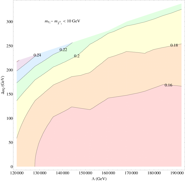
Figure 7: Contour plot of the value of $\Delta P^{2}$ obtained by fixing a particular value of $\Lambda$ and $\Delta_{PQ}$ of an F-theory GUT model with $N_{5}=1$, and minimizing with respect to all small A-term mSUGRA models. We adopt a rough criterion for theoretical distinguishability specified by the requirement that $\Delta P^{2}>0.01$. By inspection, $\Delta P^{2}$ is greater than $0.15$, indicating that such models are distinguishable at the theoretical level from F-theory GUTs. See figure 31 in Appendix F for a similar plot for $N_{5}=3$ F-theory GUTs.

As a first check, we first show to what extent these models are distinguishable as distinct particle physics models. To this end, we have computed the value of $\Delta P^{2}$ between F-theory GUT models and mSUGRA(SA) models. To gauge the level of distinguishability in the “worst case scenario”, we next minimized $\Delta P^{2}$ over all such mSUGRA(SA) models:

$$P_{SA}\left(N_{5},\Lambda,\Delta_{PQ}\right)=\underset{m_{\text{mSUGRA(SA)}}}{\min}\Delta P^{2}(m_{F},m_{\text{mSUGRA(SA)}})\text{,}$$ (49)

scanning over the parameters $M_{1/2}$, $m_{0}$, $A$ and $\tan\beta$ over the range of small A-terms specified in Appendix A. For a generic F-theory GUT model, the value of $P_{SA}$ satisfies the inequality:

$$P_{SA}\left(N_{5},\Lambda,\Delta_{PQ}\right)\gtrsim 0.15\text{.}$$ (50)

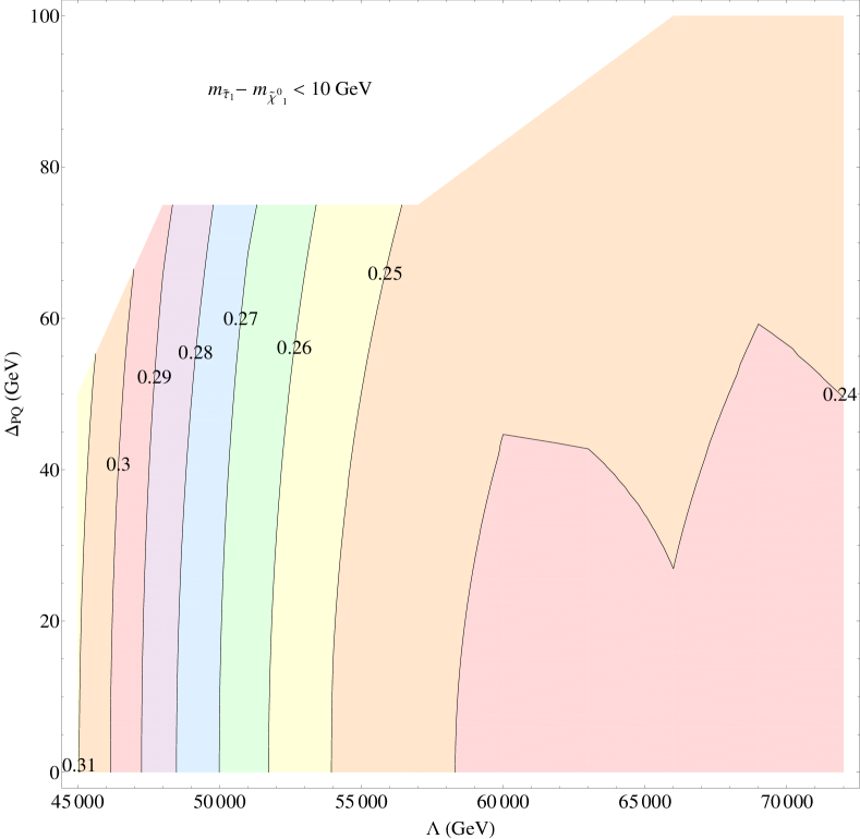
Figure 31: Contour plot of the value of $\Delta P^{2}$ obtained by fixing a particular value of $\Lambda$ and $\Delta_{PQ}$ of an F-theory GUT model with $N_{5}=3$, and minimizing with respect to all small A-term mSUGRA models. We adopt a rough criterion for theoretical distinguishability specified by the requirement that $\Delta P^{2}>0.01$. By inspection, $\Delta P^{2}$ is greater than $0.2$, indicating that such models are distinguishable at the theoretical level from F-theory GUTs.

See figure 7, and figure 31 in Appendix F for contour plots of the one and three messenger F-theory GUT models. In some sense, this level of distinguishability is to be expected, because mSUGRA models typically exhibit a more compressed spectrum where the masses of the squarks and sleptons are more degenerate. The fact that in gauge mediation models, there is more separation in the mass of the squarks, sleptons and gauginos reflects this difference.

Having established that at a theoretical level it is possible to distinguish between F-theory GUTs and small A-term mSUGRA models, we now determine experimental observables which discriminate between these two classes of models.

3.5.1 Footprint Analysis

In this subsection we use the general footprint method described earlier to compare the signatures of F-theory GUTs with small A-term mSUGRA models. To this end, we have computed LHC signatures from the models simulated using PGS. Upon constructing a footprint for these models, we next compare correlations of different pairs of signatures by making two dimensional plots. From these plots, we can distinguish at a qualitative level between F-theory models and small A-term mSUGRA models. In particular, for certain pairs of signatures, there is little to no overlap between the two classes of models. See the plots in figure 8 for examples of such signature plots. We find that signatures which distinguish between the two classes of models typically include b-jets and $\tau$ leptons.

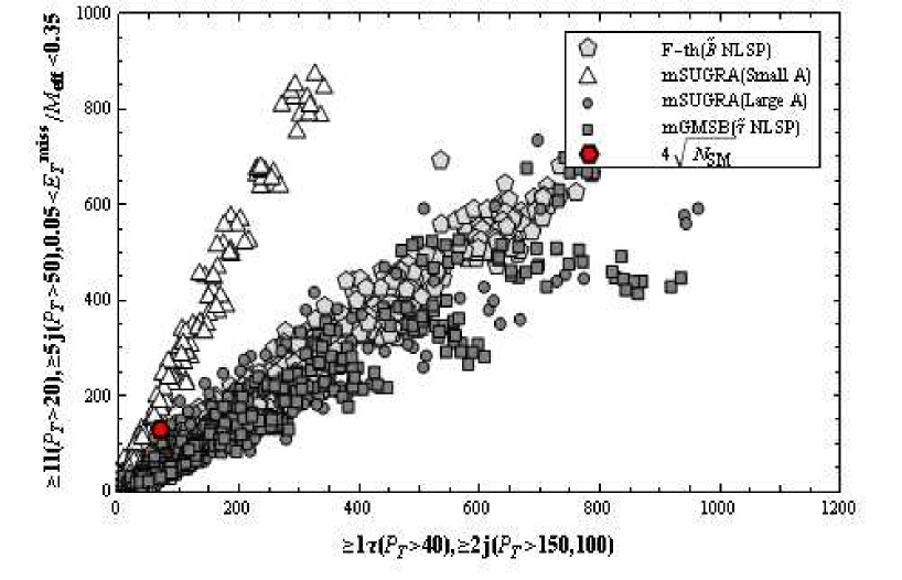
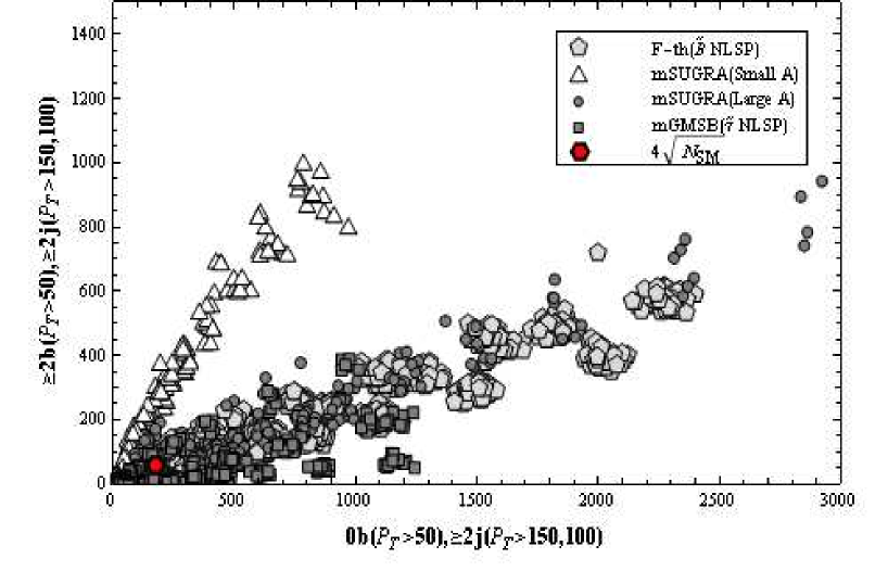
Figure 8: Footprint of LHC signatures (without SM background) for distinguishing F-theory GUTs and small A-term mSUGRA models with $5$ fb^-1 integrated luminosity. The red circle denotes the $4\sigma$ deviation from the SM background.

The differences in LHC signatures between these classes of models can be understood based on their different spectra. As mentioned before, F-theory GUTs have a light $\tilde{\tau}_{1}$, and so in models with a bino NLSP, the subsequent decay of the $\tilde{\tau}_{1}$ will produce more events with taus compared to electrons and muons. Additional leptons will be generated through the decays of the $Z$, $h$ and $t$.

This is to be contrasted with the case of small A-term mSUGRA models where leptons typically do not originate from the decay of the $\tilde{\tau}_{1}$, but rather, from the decays of the $Z$, $h$ and $t$. Since these decays are typically accompanied by b-jets, it follows that by vetoing on events with b-jets, we can expect a greater number of lepton events in F-theory GUTs in comparison with small A-term mSUGRA models. This distinction in the number of leptons to hadrons in various events explains why it is possible to distinguish between such models using signatures with taus and signatures with lepton + $0$ b-jets.

3.5.2 $\Delta S^{2}$ Analysis

We now show that with only $5$ fb^-1 of simulated LHC data, it is also possible to distinguish at a more quantitative level between F-theory GUTs and small A-term mSUGRA models. In comparing F-theory GUTs and small A-term mSUGRA models, we included all $10$ of the signatures detailed in table 2 of subsection 3.1. These signatures are not identical to the ones presented for the footprint plots, but instead appear to provide a cleaner way to minimize over $\Delta S^{2}$. We shall refer to the corresponding measure defined by signature list A as $\Delta S_{(A)}^{2}$. Much as in our discussion of $\Delta P^{2}$, we have computed the value of $\Delta S_{(A)}^{2}$ between F-theory GUTs and small A-term mSUGRA models. The value of $\Delta S_{(A)}^{2}$ between an F-theory GUT point and a typical mSUGRA point is typically far greater than $10$, and so such models are easily distinguished. However, it is still possible that certain models could share similar characteristics with F-theory GUTs. Fixing a given F-theory model, we next scanned over all of the relevant mSUGRA models, minimizing the corresponding value of $\Delta S_{(A)}^{2}$:

$$S_{SA}\left(N_{5},\Lambda,\Delta_{PQ}\right)=\underset{m_{\text{mSUGRA(SA)}}}{\min}\Delta S_{(A)}^{2}(m_{F},m_{\text{mSUGRA(SA)}})\text{,}$$ (51)

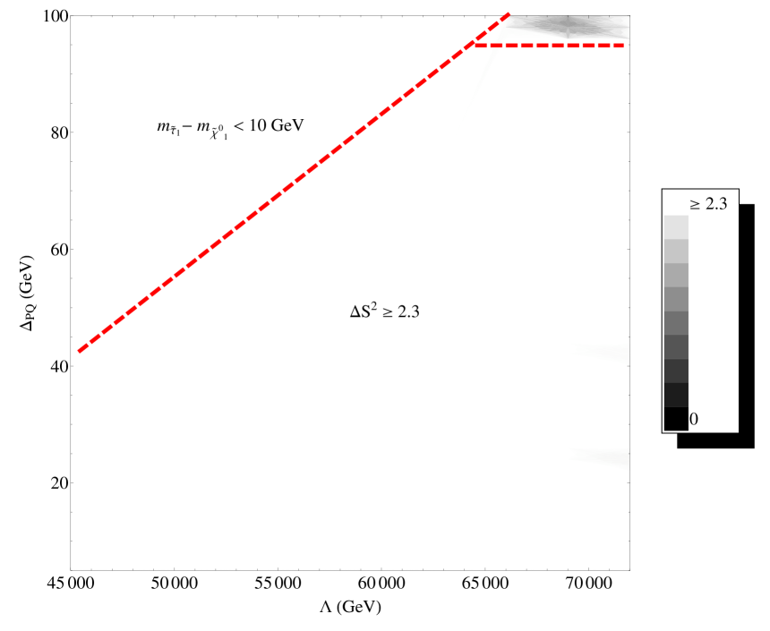
Figure 32: Density plot of $\Delta S_{(A)}^{2}$ defined by the signature list in table 2 of subsection 3.1 comparing the minimal value of a given $N_{5}=3$ F-theory GUT model with a scan over small A-term mSUGRA models. The signals used are obtained with $5$ fb^-1 of simulated LHC data. Here, we have used a rough notion of distinguishability based on $99\%$ confidence and $10$ signals so that at $\Delta S_{(A)}^{2}>2.3$ we shall say that two models are distinguishable. By inspection, for most of the plot, it is possible to distinguish between F-theory GUTs and mSUGRA models. See figure 9 in section 3 for a similar plot in the case of $N_{5}=1$ F-theory GUTs.

where here, the minimization is performed over all small A-term mSUGRA models of potential interest. See figure 9 and figure 32 in Appendix F for density plots of $S_{SA}$ for $N_{5}=1$ and $3$ as a function of $\Lambda$ and $\Delta_{PQ}$ at $5$ fb^-1 of LHC data. A similar result holds in the case of two messenger F-theory GUT models.

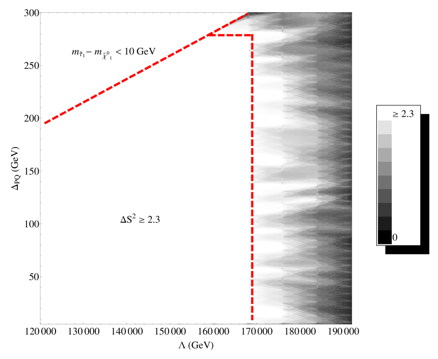
Figure 9: Density plot of $\Delta S_{(A)}^{2}$ defined by the signature list in table 2 of subsection 3.1 comparing the minimal value of a given $N_{5}=1$ F-theory GUT model with a scan over small A-term mSUGRA models. The signals used are obtained with $5$ fb^-1 of simulated LHC data. Here, we have used a rough notion of distinguishability based on $99\%$ confidence and $10$ signals so that at $\Delta S_{(A)}^{2}>2.3$ we shall say that two models are distinguishable. By inspection, for most of the plot, it is possible to distinguish between F-theory GUTs and mSUGRA models. See figure 32 in Appendix F for a similar plot in the case of $N_{5}=3$ F-theory GUTs.

These plots illustrate that it is typically possible to distinguish between F-theory GUTs and mSUGRA models. It is only by minimizing over all such points that we even come close to saturating the cutoff for distinguishability. In a certain sense, this is to be expected because the spectra and branching fractions are typically different in such models, so that in principle, there should exist signals which distinguish between these two possibilities.

3.6 F-theory Versus Large A-term mSUGRA

In the previous subsection we found that it is indeed possible to distinguish between small A-term mSUGRA models and F-theory GUTs. Large A-term mSUGRA models (mSUGRA(LA)) can also potentially mimic F-theory GUTs. Indeed, since the universal trilinear term in mSUGRA models couples the scalars of the theory, when the Higgs develops a vev, this will induce a shift in the soft masses. This by itself is important, because it can allow mSUGRA models to mimic the effects of the PQ deformation. On the other hand, introducing a large A-term changes the branching fractions in the decay of scalars. Thus, one might hope that even if the the mass spectra are somewhat similar, the decay channels in large A-term mSUGRA models could still be distinguished from F-theory GUTs.

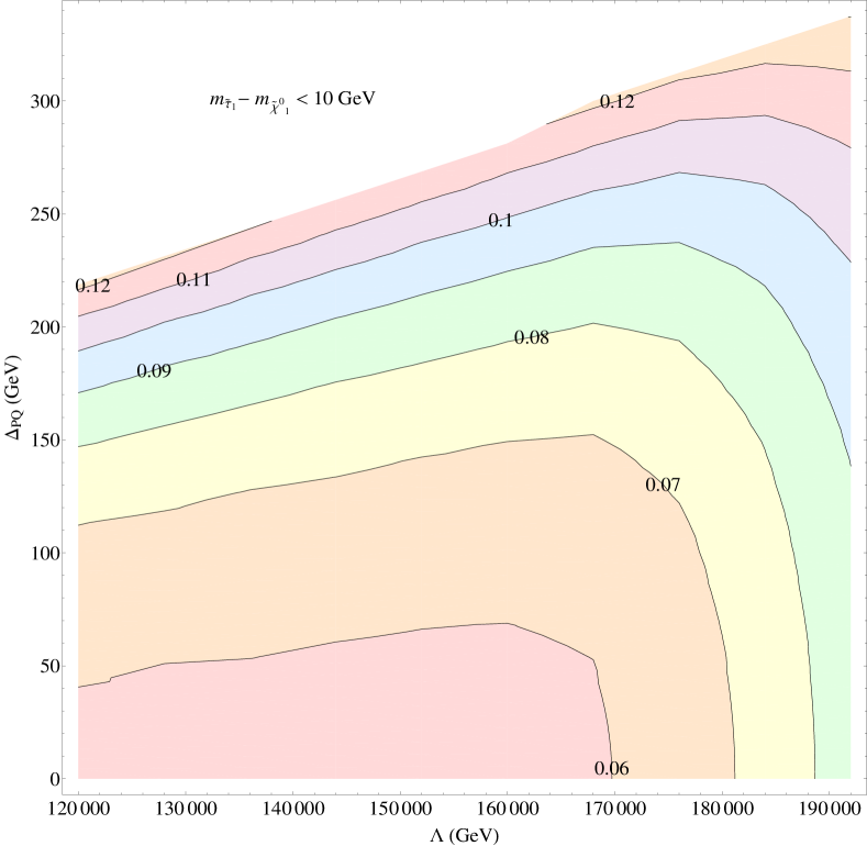
Figure 10: Contour plot of the value of $\Delta P^{2}$ obtained by fixing a particular value of $\Lambda$ and $\Delta_{PQ}$ of an F-theory GUT model with $N_{5}=1$, and minimizing with respect to all large A-term mSUGRA models. We adopt a rough criterion for theoretical distinguishability specified by the requirement that $\Delta P^{2}>0.01$. By inspection, $\Delta P^{2}$ is greater than $0.05$. This is to be contrasted with the level of distinguishability found for small A-term mSUGRA models where $\Delta P^{2}$ is greater than $0.15$. See figure 33 in Appendix F for a similar plot for F-theory GUTs with $N_{5}=3$.

To a certain extent, it is indeed possible to distinguish at a theoretical level to distinguish mSUGRA(LA) and F-theory GUT scenarios, although in comparison with small A-term models, the soft terms are closer to those of F-theory GUTs. Fixing a given F-theory GUT model, and minimizing over all mSUGRA(LA) models, we define:

$$P_{LA}\left(N_{5},\Lambda,\Delta_{PQ}\right)=\underset{m_{\text{mSUGRA(LA)}}}{\min}\Delta P^{2}(m_{F},m_{\text{mSUGRA(LA)}})\text{.}$$ (52)

we have computed the value of $P_{LA}$ for one, two and three messenger models.

In comparison to the case of small A-term mSUGRA models, the value of $P_{LA}$ is typically somewhat smaller, but is still bounded below by:

$$P_{LA}\left(N_{5},\Lambda,\Delta_{PQ}\right)\gtrsim 0.05\text{.}$$ (53)

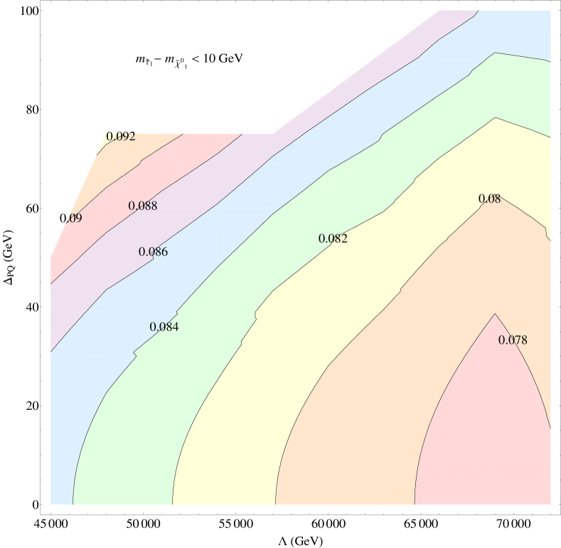
Figure 33: Contour plot of the value of $\Delta P^{2}$ obtained by fixing a particular value of $\Lambda$ and $\Delta_{PQ}$ of an F-theory GUT model with $N_{5}=3$, and minimizing with respect to all large A-term mSUGRA models. We adopt a rough criterion for theoretical distinguishability specified by the requirement that $\Delta P^{2}>0.01$. By inspection, $\Delta P^{2}$ is greater than $0.05$. This is to be contrasted with the level of distinguishability found for small A-term mSUGRA models where $\Delta P^{2}$ is greater than $0.15$.

Figure 10 and figure 33 in Appendix F show contour plots of $P_{LA}$ as a function of $\Lambda$ and $\Delta_{PQ}$. Note that in comparison to the small A-term mSUGRA model contour plots depicted in figure 7 and figure 31 in Appendix F, the soft parameters of this class of models can more effectively mimic F-theory GUTs.

3.6.1 Footprint Analysis

In this section, we discuss whether the footprints of large A-term mSUGRA and F-theory GUTs can be used to distinguish these two classes of models. As before, we generated two dimensional footprints using the $103$ signatures listed in Appendix C. By inspecting many footprint plots, we have found a few signatures which can be used to distinguish F-theory GUTs and large A-term mSUGRA models as in figure 11. These plots also show that there is still a large overlap in the region corresponding to models with relatively small cross section. The primary overlap region is mainly comprised of two and three messenger F-theory GUT models. For this reason, we find that it is not possible to cleanly distinguish F-theory GUTs with multiple messengers in the bino NLSP regime from large A-term mSUGRA models with our implementation of signatures and limited integrated luminosity. We also notice that the simple signatures involving lepton as well as tau and b-jet cannot distinguish these two classes of models. As we shall explain in greater detail in subsection 3.6.3, this can be roughly understood from the fact that the two and three messenger F-theory GUT models

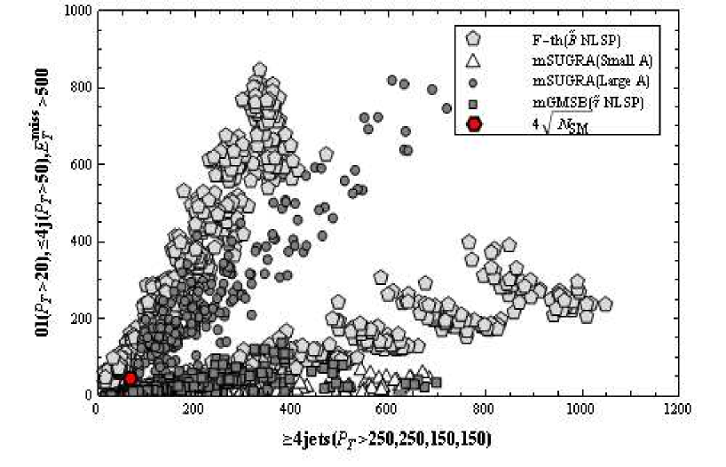
Figure 11: Footprint of LHC signatures (without SM background) for distinguishing F-theory GUTs and large A-term mSUGRA models with $5$ fb^-1 integrated luminosity. The red circle denotes the $4\sigma$ deviation from the SM background.

share the same decay topology with large A-term mSUGRA models. For the two messenger case, there are differences in the lightest stau and Higgsino mass in the region of small $\Lambda$. Nevertheless, these distinctions do not seem to be sufficient for producing discriminating LHC signatures with $5$ fb^-1 of LHC data. On the other hand, figure 11 illustrates that multi-jet signatures partially resolve this “degeneracy”. This could be due to the difference in the branching ratio of gluino decay into tops and stops.

3.6.2 $\Delta S^{2}$ Analysis

In this section we discuss the extent to which F-theory GUTs can be distinguished from large A-term mSUGRA models. We find that although single messenger models can typically be distinguished from such large A-term scenarios, in the case of two and three messengers, the value of $\Delta S^{2}$ does not effectively distinguish between all such F-theory GUTs and large A-term mSUGRA (mSUGRA(LA)) models. As in the case of the small A-term mSUGRA models, we have used the $10$ signatures detailed in table 2 of subsection 3.1. We find that there is typically a small region at small and large $\Lambda$ where it is possible to distinguish multiple messenger F-theory GUT models from mSUGRA(LA) models. Although in many cases the value of $\Delta S_{(A)}^{2}$ between F-theory GUTs and mSUGRA(LA) models is on the order of $10$ or more, other mSUGRA(LA) models can effectively mimic the signatures of F-theory GUTs.

Figure 12: Density plot of $\Delta S_{(A)}^{2}$ defined by the signature list in table 2 of subsection 3.1 comparing the minimal value of a given $N_{5}=1$ F-theory GUT model with a scan over large A-term mSUGRA models. The signals used are obtained with $5$ fb^-1 of simulated LHC data. Here, we have used a rough notion of distinguishability based on $99\%$ confidence and $10$ signals so that at $\Delta S_{(A)}^{2}>2.3$ we shall say that two models are distinguishable. The plot shows the minimal value of $\Delta S^{2}$ for a fixed F-theory GUT point. By inspection, we see that just as for the small A-term case, single messenger F-theory GUTs can be distinguished from mSUGRA models over much of the range of interest. This is in contrast to the case of multiple messenger models where the same signatures do not cleanly distinguish between F-theory and mSUGRA(LA) models. See figures 34 and 35 of Appendix F for the analogous plots in the multiple messenger case.

To quantify the extent to which F-theory GUTs can be distinguished from such models, we have computed the value of the function:

$$S_{LA}\left(N_{5},\Lambda,\Delta_{PQ}\right)=\underset{m_{\text{mSUGRA(LA)}}}{\min}\Delta S_{(A)}^{2}(m_{F},m_{\text{mSUGRA(LA)}})$$ (54)

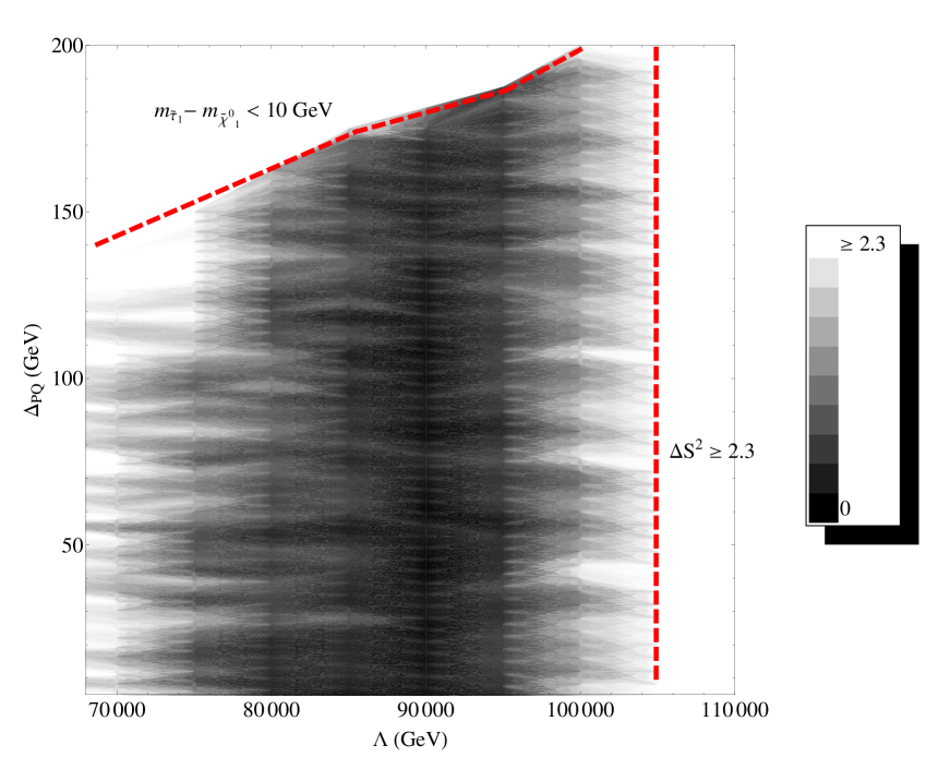
Figure 34: Density plot of $\Delta S_{(A)}^{2}$ defined by the signature list in table 2 of subsection 3.1 comparing the minimal value of a given $N_{5}=2$ F-theory GUT model with a scan over large A-term mSUGRA models. The signals used are obtained with $5$ fb^-1 of simulated LHC data. Here, we have used a rough notion of distinguishability based on $99\%$ confidence and $10$ signals so that at $\Delta S_{(A)}^{2}>2.3$ we shall say that two models are distinguishable. The plot shows the minimal value of $\Delta S^{2}$ for a fixed F-theory GUT point. This plot shows that for this class of signatures, the models are only distinguishable at larger values of $\Lambda$.

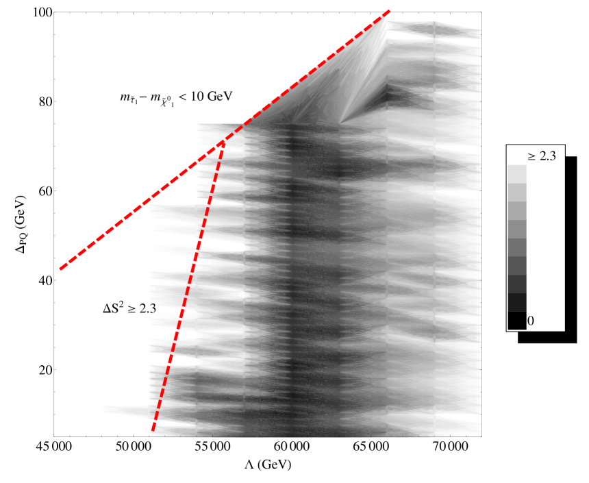
Figure 35: Density plot of $\Delta S_{(A)}^{2}$ defined by the signature list in table 2 of subsection 3.1 comparing the minimal value of a given $N_{5}=3$ F-theory GUT model with a scan over large A-term mSUGRA models. The signals used are obtained with $5$ fb^-1 of simulated LHC data. Here, we have used a rough notion of distinguishability based on $99\%$ confidence and $10$ signals so that at $\Delta S_{(A)}^{2}>2.3$ we shall say that two models are distinguishable. This plot shows that for this class of signatures, the models are only distinguishable at small values of $\Lambda$.

obtained by minimizing over all large A-term mSUGRA models of interest. Figure 12 shows that for $N_{5}=1$, typically $S_{LA}>2.3$. On the other hand, figures 34 and 35 in Appendix F show that for $N_{5}=2$ and $N_{5}=3$, it is more difficult to distinguish F-theory GUTs from large A-term scenarios.

3.6.3 More on the Multiple Messenger Case

In the previous subsections we found that single messenger F-theory GUT models are distinguishable from large A-term mSUGRA models, both at the level of footprint plots and at a semi-quantitative level using the measures $\Delta S^{2}$. On the other hand, the large A-term mSUGRA models appear to more effectively mimic the multiple messenger F-theory GUTs with a bino NLSP. In this subsection we discuss some further features of such models which partially explain the observed overlaps in signatures.

Because of the similarity in the stau and neutralino masses, the decay of $\widetilde{\chi}_{2}^{0}$ via an on-shell $\tilde{\tau}_{1}$ can enable large A-term models to mimic the leptonic signals of F-theory GUTs. Figure 13 shows the value of the LSP mass versus the branching ratio $\tilde{\chi}_{2}^{0}\rightarrow\tilde{\tau}_{1}+\tau$ for a range of mSUGRA(LA) models. The large variation in values implies that such models can effectively mimic the value of the branching fraction present in F-theory GUTs. Further, although we have seen that single messenger models can indeed be distinguished from mSUGRA(LA) models, some of the parameters of such models such as the masses of the lightest neutralinos $\tilde{\chi}_{1}^{0}$ and $\tilde{\chi}_{2}^{0}$ are quite similar. Figure 14 shows that the mass of the lightest stau can essentially cover the entire range of values between $m_{\tilde{\chi}_{1}^{0}}$ and $m_{\tilde{\chi}_{2}^{0}}$. Note, however, that at smaller values of the neutralino mass, a gap exists in the range of values for the lightest stau mass. Since multiple messenger F-theory GUTs with a bino NLSP typically have a $\tilde{\tau}_{1}$ which is close in mass to $\tilde{\chi}_{1}^{0}$, this difference may lead to observable differences between multiple messenger F-theory GUTs and mSUGRA(LA) models.

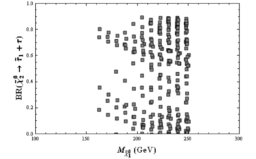
Figure 13: Plot of second neutralino branching fraction $\widetilde{\chi}_{2}^{0}\rightarrow\widetilde{\tau}_{1}^{\pm}+\tau^{\mp}$ in large A-term mSUGRA models versus the LSP mass. The large distribution of values indicates that such models can effectively mimic the branching fraction present in other models, such as F-theory GUTs. Note, however, that there is a gap in the lower left part of the distribution. The relation between the mass of the stau and the two lightest neutralinos in this region is similar to that of two and three messenger F-theory GUTs with a bino NLSP.

Large A-term models can also mimic F-theory GUT signals controlled by the decay of colored particles. In large mSUGRA(LA) models, the main decay channels for the gluino are $\tilde{g}\rightarrow\tilde{t}_{1}t$, $\tilde{g}\rightarrow\tilde{b}_{1}b$ and $\tilde{g}\rightarrow\tilde{b}_{2}b$. See figure 15 for a plot of each of these branching ratios. The total branching ratio into third generation quarks is around $90\%$. Since the gluino decay is a two-body process, multi-jets plus missing $E_{T}$ signature should distinguish these mSUGRA models with single messenger F-theory GUTs, as we have already seen. Indeed, this is consistent with the discussion in section 2 that the gluino decays via a three-body process in single messenger models. Note, however, that in two and three messenger F-theory GUTs, the gluino decay is also a two body process and is quite similar to large A-term mSUGRA models. In fact, the total branching ratio to third generation squarks and quarks is respectively $100\%$ and $80\%$. This explains why simple b-jet counting does not help in distinguishing between F-theory models and large A-term mSUGRA models.

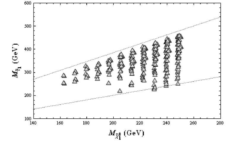
Figure 14: Plot of the mass of the lightest stau in large A-term mSUGRA models versus the LSP mass. The upper line in the plot corresponds to $m_{\tilde{\chi}_{2}^{0}}$, while the lower one corresponds to $m_{\tilde{\chi}_{1}^{0}}$. By inspection, the mass of the $\widetilde{\tau}_{1}$ effectively covers the entire range between the mass of $\widetilde{\chi}_{1}^{0}$ and $\widetilde{\chi}_{2}^{0}$, so that such models can effectively mimic the mass hierarchy present in F-theory GUTs.

Further note that for two messenger F-theory GUTs, there is a larger branching ratio to $\tilde{t}_{1}t$, which is, however, not present in the three messenger case. At first, this would seem to provide a promising class of processes to focus on since the increase in the number of top quarks from gluino decay will leads to an increase in the number of $W$ bosons, which would seemingly produce a sizable difference in the lepton signatures. Unfortunately, the heavy neutralinos $\widetilde{\chi}_{3,4}^{0}$ are generally lighter in F-theory models, and thus give rise to softer gauge bosons and subsequently produced leptons. This leads to opposite effects on the lepton signatures compared to the large $\tilde{t}_{1}t$ branching ratio. Therefore, at least in the case of low integrated luminosity, distinguishing F-theory models with two and three messenger from large A-term mSUGRA models appears to be much more challenging at the LHC.

To further distinguish between large A-term scenarios and F-theory GUTs, increased luminosity will certainly help (see for example equation (38) of subsection 3.1). At the same time, one could look for signatures which are sensitive to the $\tilde{t}_{1}t$ channel of gluino decay. In addition, $\tan\beta$ enhanced signatures could also be useful, since, as figure 16 shows, large A-term mSUGRA models typically have larger $\tan\beta$ than F-theory GUTs. An effective observable may come from rare B-decays such as $B_{s}\rightarrow\mu^{+}\mu^{-}$ where the additional gluino contribution to the decay rate can be significantly enhanced by a factor proportional to $\tan^{6}\beta$ in the large $\tan\beta$ regime (see [44] for a recent study). However, a full analysis of these possibilities is beyond the scope of this paper, and we leave this issue for future investigations.

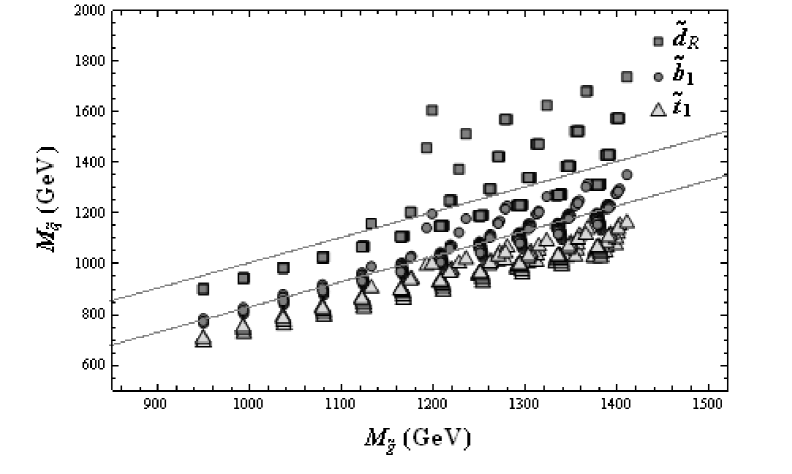
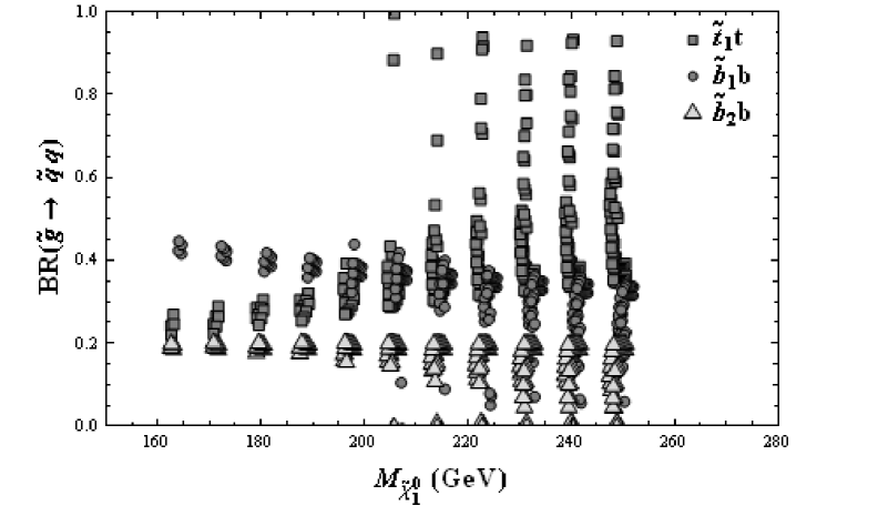
Figure 15: Top figure: the squark mass distribution $(\tilde{t}_{1},\tilde{b}_{1},\tilde{d}_{R})$ in large A-term mSUGRA models. The upper line corresponds to $m_{\tilde{g}}$ and the lower line to $m_{\tilde{g}}-m_{t}$. Bottom figure: the gluino branching fraction in large A-term mSUGRA models versus the LSP mass in the decay channels $\widetilde{g}\rightarrow\widetilde{t}_{1}+t$, $\widetilde{g}\rightarrow\widetilde{b}_{1}+b$, and $\widetilde{g}\rightarrow\widetilde{b}_{2}+b$.

Beyond collider signatures, astrophysical probes could provide another means by which to distinguish large A-term mSUGRA models from multiple messenger F-theory GUTs. In mSUGRA models, the lightest neutralino provides a natural dark matter candidate. This is in contrast to the situation in F-theory GUTs where the neutralino is unstable, eventually decaying to a gravitino LSP. The difference in the nature of the LSP will affect the dark matter relic density. For example, in the bino LSP case, generating an acceptable dark matter relic density from binos requires a light stau which is almost degenerate in mass with the LSP. This further criterion would exclude most of the large A-term mSUGRA models in our study, thus providing better separation between F-theory GUTs and large A-term models. In addition, both direct and indirect dark matter detection experiments can potentially see evidence of a neutralino LSP, but not gravitinos. Therefore, non-collider signature could provide an additional means by which to distinguish F-theory GUTs and mSUGRA models.

Figure 16: Plot of $\tan\beta$ in large A-term mSUGRA models versus the mass of the LSP. This is to be compared with the values of $\tan\beta$ in F-theory GUTs which have been overlaid on the same plot as a function of $\Lambda$ (axis not shown). The $N_{5}=3$ case is omitted because it is similar to the $N_{5}=2$ case. This plot shows that the value of $\tan\beta$ in large A-term mSUGRA models is typically larger than that in F-theory GUTs. In particular, $\tan\beta$ enhanced processes could therefore potentially distinguish between F-theory GUTs and such mSUGRA models.

3.7 F-theory Versus Low Scale mGMSB

In this subsection we compare F-theory GUTs with minimal GMSB scenarios with a low messenger scale, deferring a comparison with high messenger scale scenarios to section 4. Returning to the discussion near (41), recall that a stau NLSP low scale mGMSB model can potentially mimic some of the signatures of F-theory GUTs with a bino NLSP. Indeed, all other scenarios have qualitatively distinct behavior, and so we shall focus on this one remaining case.

Figure 17: Contour plot of the value of $\Delta P^{2}$ obtained by fixing a particular value of $\Lambda$ and $\Delta_{PQ}$ of an F-theory GUT model with $N_{5}=1$, and minimizing with respect to all low scale minimal GMSB models with a stau NLSP. We adopt a rough criterion for theoretical distinguishability specified by the requirement that $\Delta P^{2}>0.01$. By inspection, $\Delta P^{2}$ is greater than $0.1$, indicating that such models are distinguishable at the theoretical level from F-theory GUTs. See figure 36 in Appendix F for a similar plot for $N_{5}$ = 3 F-theory GUTs.

Even though the presence of signatures with missing $E_{T}$ can potentially be mimicked, there are still important differences in both the soft parameters, and collider signatures. As in our comparison with mSUGRA models, we have scanned over low scale mGMSB models with a stau NLSP (see Appendix B for a description of this scan), and computed the value of $\Delta P^{2}$ between these models and F-theory GUTs. Minimizing over all such models, we have determined the value of

$$P_{LO}\left(N_{5},\Lambda,\Delta_{PQ}\right)=\underset{m_{\text{mGMSB(LO)}}}{\min}\Delta P^{2}(m_{F},m_{\text{mGMSB(LO)}})\text{.}$$ (55)

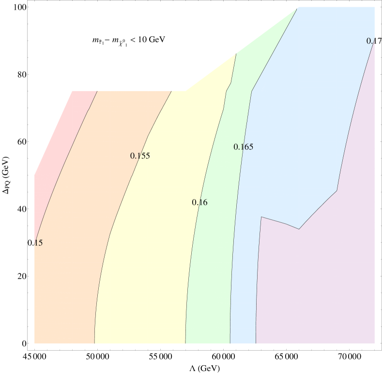
Figure 36: Contour plot of the value of $\Delta P^{2}$ obtained by fixing a particular value of $\Lambda$ and $\Delta_{PQ}$ of an F-theory GUT model with $N_{5}=3$, and minimizing with respect to all low scale minimal GMSB models with a stau NLSP. We adopt a rough criterion for theoretical distinguishability specified by the requirement that $\Delta P^{2}>0.01$. By inspection, $\Delta P^{2}$ is greater than $0.15$, indicating that such models are distinguishable at the theoretical level from F-theory GUTs.

Figure 17 and figure 36 in Appendix F show contour plots of $P_{LO}$ as a function of $\Lambda$ and $\Delta_{PQ}$. These plots illustrate that

$$P_{LO}\gtrsim 0.1\text{.}$$ (56)

It is interesting to note that although both classes of models share the same mechanism for the mediation of supersymmetry breaking, the soft terms of large A-term mSUGRA models can more effectively mimic the soft terms of F-theory GUTs. Having established this distinction, we now discuss footprints which distinguish between the signatures of these two classes of models.

3.7.1 Footprint Analysis

The footprint of low scale mGMSB models with a stau NLSP can be easily separated from that of F-theory GUTs by using $0\tau$ and $\geq 2\tau$ signatures as seen in figure 18. As explained in section 3.2, this is because there exist long decay chains where the lightest neutralinos decay into a stau and then to a gravitino, leading to events with many taus.

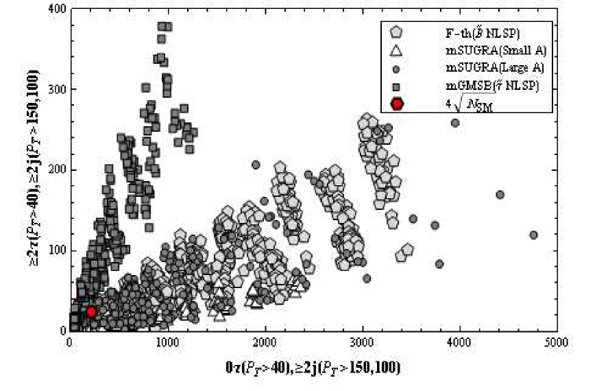
Figure 18: Footprint of LHC signatures (without SM background) for distinguishing F-theory GUTs and low scale mGMSB models with a stau NLSP with $5$ fb^-1 integrated luminosity. The red circle denotes the $4\sigma$ deviation from the SM background.

3.7.2 $\Delta S^{2}$ Analysis

Having seen that the footprints of F-theory GUTs are quite distinct from low scale mGMSB models, we next compute using the same $10$ signatures detailed in table 2 of subsection 3.1 the value of $\Delta S_{(A)}^{2}$ between these two classes of models. Minimizing over all such low scale models, we define the function:

$$S_{LO}\left(N_{5},\Lambda,\Delta_{PQ}\right)=\underset{m_{\text{mGMSB(LO)}}}{\min}\Delta S_{(A)}^{2}(m_{F},m_{\text{mGMSB}})\text{.}$$ (57)

In this case, we find that over the entire range of parameters scanned for $\Lambda$ and $\Delta_{PQ}$,

$$S_{LO}\left(N_{5},\Lambda,\Delta_{PQ}\right)\geq 2.3$$ (58)

when $N_{5}=2,3$. This is the threshold for distinguishability at $99\%$ confidence, and so we find that it is relatively easy to distinguish between these models. Moreover, figure 19 shows that even in the case of single messenger F-theory GUT models, much of the range of F-theory GUTs is distinguishable using these same signatures. This illustrates that in general, we can expect to distinguish between F-theory GUTs and low scale mGMSB models.

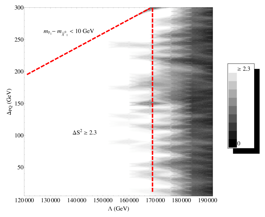
Figure 19: Density plot of $\Delta S_{(A)}^{2}$ defined by the signature list in table 2 of subsection 3.1 comparing the minimal value of a given $N_{5}=1$ F-theory GUT model with a scan over low scale mGMSB models with a stau NLSP. The signals used are obtained with $5$ fb^-1 of simulated LHC data. Here, we have used a rough notion of distinguishability based on $99\%$ confidence and $10$ signals so that at $\Delta S_{(A)}^{2}>2.3$ we shall say that two models are distinguishable. By inspection, much of the scanned region of F-theory GUTs is distinguishable from such models.

4 Determination of F-theory Parameters

In this section we determine the extent to which two distinct F-theory GUT models can be distinguished from one another. Note that since high messenger scale mGMSB models correspond to a subclass of F-theory GUTs with $\Delta_{PQ}=0$, performing this analysis will also address whether F-theory GUTs can be distinguished from a minimal GMSB model with a high messenger scale.

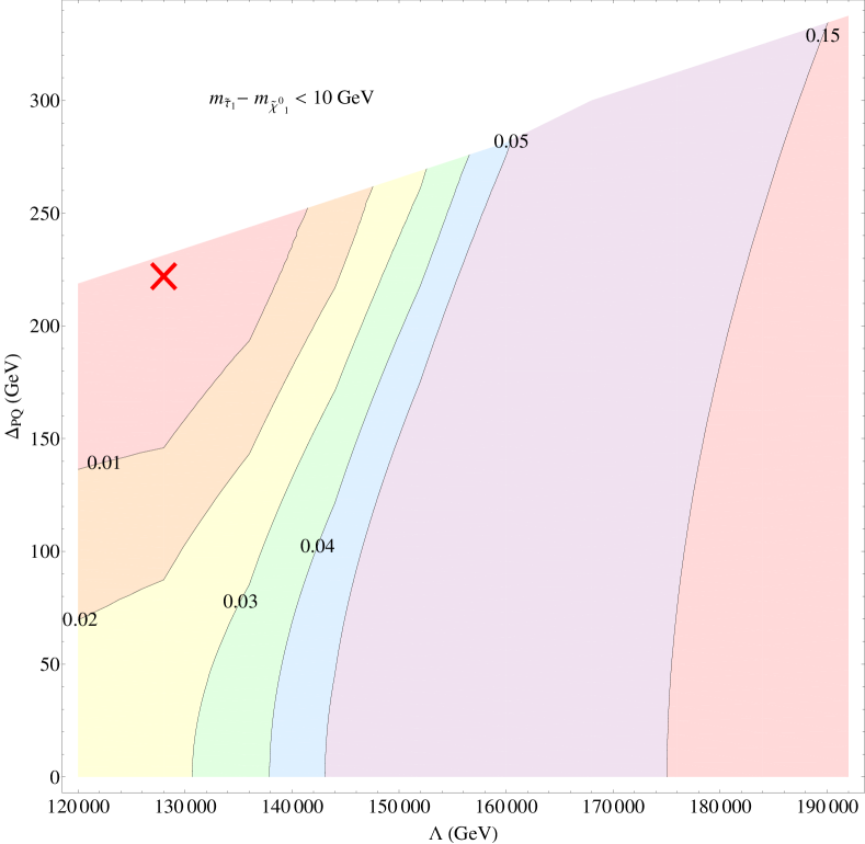
Figure 20: Contour plot of $\Delta P^{2}$ between a fixed F-theory GUT model with $N_{5}=1$, $\Lambda=1.28\times 10^{5}$ GeV and $\Delta_{PQ}=222$ GeV (indicated by red X), and single messenger F-theory GUT models. We adopt a rough criterion for theoretical distinguishability specified by the requirement that $\Delta P^{2}>0.01$. This figure shows that $\Delta P^{2}$ minimizes in the vicinity of the representative point, and that in particular, there is no degeneracy in the soft terms in a scan over single messenger models. However, figure 37 of Appendix F shows that in plots of $\Delta P^{2}$ between this point and three messenger models, there are still regions where a local minimum is potentially possible, although this value is greater than $0.02$.

Using the same $\Delta P^{2}$ measure of theoretical distinguishability based on soft terms utilized earlier, we have computed the value of $\Delta P^{2}$ between a fixed F-theory GUT specified by the parameters $N_{5}^{(0)},\Lambda^{(0)},\Delta_{PQ}^{(0)}$, and the class of all F-theory GUTs:

$$P_{FTH}\left(N_{5},\Lambda,\Delta_{PQ}\right)=\Delta P^{2}(m_{F}(N_{5}^{(0)},\Lambda^{(0)},\Delta_{PQ}^{(0)}),m_{F}(N_{5},\Lambda,\Delta_{PQ}))\text{.}$$ (59)

We find that for each $N_{5}$, $P_{FTH}$ achieves a local minimum only for a small strip of values of $\Lambda$, which typically extends over a range of values for $\Delta_{PQ}$. However, the absolute minimum of $P_{FTH}$ is always smaller when $N_{5}=N_{5}^{(0)}$. Typically, single messenger models are more easily distinguished from multiple messenger models since the spectrum and soft terms of single messenger F-theory GUTs are distinct. For example, in single messenger models, some of the squarks are typically heavier than the gluino, whereas in multiple messenger models, the gluino is always heavier. Due to the similarities in the sparticle spectrum, two and three messenger F-theory GUTs can exhibit similar behavior.

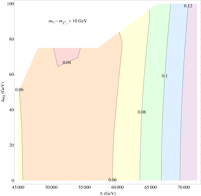
Figure 37: Contour plot of $\Delta P^{2}$ between a fixed F-theory GUT model with $N_{5}=1$, $\Lambda=1.28\times 10^{5}$ GeV and $\Delta_{PQ}=222$ GeV and three messenger F-theory GUT models. We adopt a rough criterion for theoretical distinguishability specified by the requirement that $\Delta P^{2}>0.01$. This figure shows that $\Delta P^{2}$ minimizes in the vicinity of a small patch. However, it should be noted that there is no contour for $\Delta P^{2}=0.03$ because the resulting scan typically saturates above this value. This is in accord with the fact that the fixed F-theory GUT and the models scanned have a different number of messenger fields.

Fixing a representative single messenger model with $\Lambda^{(0)}=1.28\times 10^{5}$ GeV and $\Delta^{(0)}_{PQ}=222$ GeV as the “LHC point”, figure 20 shows that in a scan over all single messenger models, there is a single local minimum for $\Delta P^{2}$. In addition, while there is certainly a similar local minimum present in the scan over three messenger model shown in figure 37 of Appendix F, the minimal value of $\Delta P^{2}$ in such cases is bounded below by roughly $0.03$, so that with our rough criterion, such models are distinguishable. Similar considerations apply for other representative “LHC point” with a single messenger. By contrast, figure 21 illustrates that when the “LHC point” corresponds to a two messenger model with $\Lambda^{(0)}=8\times 10^{4}$ GeV and $\Delta^{(0)}_{PQ}=104$ GeV, there exists a strip of three messenger models with $\Delta P^{2}<0.01$, which falls below the rough bound we have adopted for distinguishability. Even so, it is important to note that at no point does $\Delta P^{2}$ appear to vanish. With this in mind, the fact that $\Delta P^{2}$ can be small should be viewed as a rough guide for what to expect when searching for discriminating signatures.

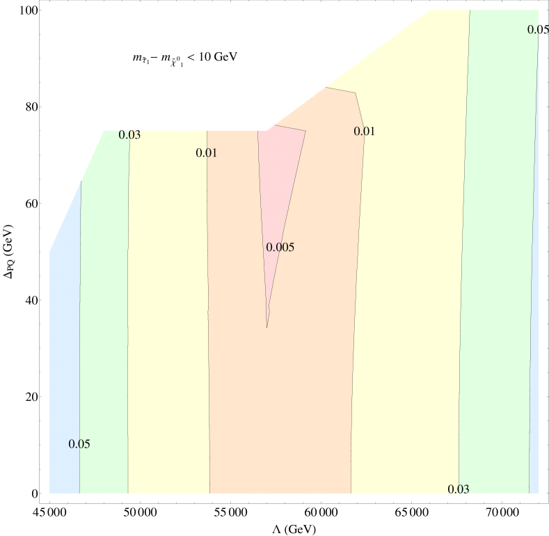
Figure 21: Contour plot of $\Delta P^{2}$ between a fixed F-theory GUT model with $N_{5}=2$, $\Lambda=8\times 10^{4}$ GeV and $\Delta_{PQ}=104$ GeV and three messenger F-theory GUT models. This figure shows that even though the number of messengers are different, the value of $\Delta P^{2}$ can minimize to a value below our rough criterion for distinguishability given by $0.01$. Note, however, that although $\Delta P^{2}<0.01$, the range of values for which $\Delta P^{2}<0.005$ is far smaller, indicating that at least in principle, two and three messenger models are distinguishable at a theoretical level.

In the remainder of this section we investigate the extent to which different F-theory GUTs generate distinguishable experimental signatures. To this end, in subsection 4.1 we first list candidate signatures of interest which have strong dependence on the parameters of F-theory GUTs. Using these signatures, we compute the corresponding value of $\Delta S^{2}$ between a fixed “LHC point” and various F-theory GUTs. In particular, we show that this type of analysis is capable of determining both $N_{5}$ and $\Lambda$, and moreover, can distinguish between scenarios with small and large PQ deformation. Restricting to the case of single messenger F-theory GUTs and a particular value of $\Lambda$, we next compute the value of $\Delta S^{2}$ between models with different values of $\Delta_{PQ}$. We find that at $5$ fb^-1 of simulated data, $\Delta_{PQ}$ can be determined up to an uncertainty of $\sim\pm 80$ GeV, while at $50$ fb^-1, this improves to an uncertainty of $\sim\pm 10$ GeV. In particular, this shows that the LHC is indeed sensitive, albeit indirectly, to string scale physics! Finally, although outside the main focus of this paper, in Appendix E we consider the sensitivity of the endpoint of the ditau invariant mass distribution as a function of $\Delta_{PQ}$.

4.1 Signature List

We now proceed to discuss signatures which are especially sensitive to $N_{5}$, $\Lambda$ and $\Delta_{PQ}$. As explained in subsection 3.1, we have generated a total of $103$ LHC signatures for all $1530$ F-theory GUT models. However, not all of these signatures are sensitive to changes in the parameters of F-theory GUTs. In some cases, either poor statistics, or a correlation in seemingly different signatures can obstruct the use of these observables. A general discussion of selecting signatures can be found in reference [42]. As explained there, there exists some optimal choice and number of signatures which minimize the luminosity needed for distinguishing between two models. Although a systematic optimization is certainly useful, it goes beyond the scope of this paper. For our study, we will instead consider a manual selection of signatures by examining the footprint of F-theory GUTs using all possible pairs of signatures. For example, to find the signatures sensitive to $N_{5}$, we examined all possible two-dimensional plots constructed out of $103$ signatures for models with different $N_{5}$. We then selected by examining such plots a class of signatures which do not appear to share any significant correlations. One such set of signatures which are especially helpful in a footprint analysis are shown as signature list B in table 3. Figure 22 illustrates an example of some signatures which distinguish between single and multiple messenger models. Notice that the one messenger models are more easily separated from the two and three messenger models. This is consistent with the fact explained in section 2 that these models have different gluino and squark decay topologies. Similarly, we have also find a set of signatures referred to as signature list C which are sensitive to the PQ deformation parameter $\Delta_{PQ}$. Figure 23 shows two signatures as functions of $\Delta_{PQ}$. Finally, in our $\Delta S^{2}$ analysis, we have used signature list D given in table 4.

	Signature List B
1	$\geq 4$ jets($P_{T}>100,50,50,50$)
2	$\geq 6$ jets($P_{T}>150,150,100,100,50,50$)
3	$0b(P_{T}>50),\geq 2$jets($P_{T}>150,100$)
4	$\geq 2b(P_{T}>50),\geq 2$jets($P_{T}>150,100$)
5	$0l(P_{T}>20),\leq 4$jets($P_{T}>50$), $M_{eff}>1500$
	Signature List C
1	$\geq 6$jets($P_{T}>150,150,100,100,50,50$)
2	$\geq 1\tau$($P_{T}>40$),$\geq 2$jets($P_{T}>150,100$)
3	$\geq 1l$($P_{T}>40$),$\geq 4$jets($P_{T}>100,50,50,50$)
4	$0\tau$($P_{T}>10$),$\geq 4$jets($P_{T}>100,50,50,50$)
5	$\geq 1\tau$($P_{T}<40$),$\geq 2$jets($P_{T}>70$)
6	$0l$($P_{T}>20$),$\leq 4$jets($P_{T}>50$), $\displaystyle{\not}E_{T}>500$

Table 3: The collection of signatures which are effective for distinguishing models with distinct values of $N_{5}$ (List B) and $\Delta_{PQ}$ (List C) using footprint plots. All cuts are in units of GeV. Table 4 contains an alternate set of signatures which are especially helpful in distinguishing models using the $\Delta S^{2}$ measure.

	Signature List D
$1$	$\geq 4$jets($P_{T}>100,50,50,50$)
$2$	$\geq 4$jets($P_{T}>250,250,100,100$)
$3$	$\geq 2$jets($P_{T}>350,350$)
$4$	$\geq 6$jets($P_{T}>150,150,100,100,50,50$)
$5$	$0\tau$($P_{T}>20$),$\geq 4$jets($P_{T}>100,50,50,50$)
$6$	$1\tau$($P_{T}>40$),$\geq 4$jets($P_{T}>100,50,50,50$)
$7$	$1b$($P_{T}>50$),$\geq 4$jets($P_{T}>100,50,50,50$)
$8$	$0l$($P_{T}>10$),$\leq 4$jets($P_{T}>50$), $M_{eff}>1400$
$9$	$0l$($P_{T}>10$), $\leq 4$jets($P_{T}>50$), $M_{eff}>1400$, $M_{inv}({\rm jets})>800$
$10$	$0l$($P_{T}>10$), $\geq 5$jets($P_{T}>50$), $M_{eff}>1400$
$11$	$0l$($P_{T}>10$), $\geq 5$jets($P_{T}>50$), $M_{eff}>800$, $P_{T}(\textrm{4th hardest jet})>140$
$12$	$\geq 1l$($P_{T}>10$), $\geq 5$jets($P_{T}>50$), $M_{eff}>1400$
$13$	$\geq 1l$($P_{T}>10$), $\geq 5$jets($P_{T}>50$), $0.1<\displaystyle{\not}E_{T}/M_{eff}<0.3$

Table 4: The collection of LHC signatures used in our $\Delta S^{2}$ analysis. All cuts are in units of GeV. In all signatures where a cut is not explicitly stated, we have imposed a base cut of $\displaystyle{\not}E_{T}>100$ GeV and $M_{eff}>1200$ GeV

In tables 3 and 4, the corresponding signatures solely consist of inclusive multijet (with particular $P_{T}$ cuts) plus missing $E_{T}$ signatures, or signatures with one more lepton or tau (with particular $P_{T}$ cuts). This is not so surprising as most other more exclusive event selections such as those based on two or three lepton signatures have low statistics at $5$ fb^-1. Even assuming sufficient statistics, we find that in comparison with one lepton signatures, such signatures typically do not distinguish as cleanly between various models.

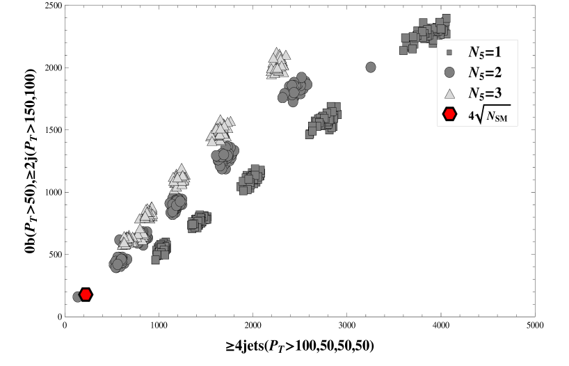
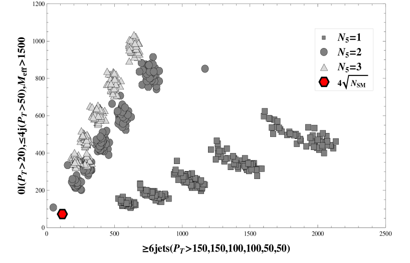
Figure 22: Footprint of F-theory models with different $N_{5}$ with $5$ fb^-1 of integrated luminosity. These plots shows the footprint can distinguish F-theory based models with different numbers of messengers $N_{5}$.

We now discuss in greater detail the signatures in table 3. The first two signatures in signature list B are multijet + missing $E_{T}$ signatures. We indicate $P_{T}$ thresholds of jets in the parentheses. The detailed selection criteria are provided in table 1 of subsection 3.1. These multijet signatures with different choices of thresholds are chosen to capture the differences in the jet multiplicity and $P_{T}$ distributions, and will thus be sensitive to the gluino and squark decays. The signatures $0b(P_{T}>50),\geq 2$ jets and $2b(P_{T}>50),\geq 2$ jets are selected by veto b-jets or requiring at least two b-jets with $P_{T}$ threshold given in the parentheses from the inclusive selections $\geq 2$jets($P_{T}>150,100$). The remaining signatures in list B are $0l(P_{T}>20),\leq 4$jets($P_{T}>50$) with $M_{eff}>1500$. For signature list C, the signatures are basically inclusive signatures with one lepton, one tau and multijets. The reason why these signatures are sensitive to $\Delta_{PQ}$ can be traced back to the shift in the masses of $\tilde{t}_{1}$ and $\tilde{\tau}_{1}$, though the detail reason could be complicated due to the mixture of different production and decay channels. Similar considerations apply for signature list D in table 4. Here, it is important to stress that different analyses are better suited to different sets of signatures. For example, in our footprint analysis, we find that signatures from table 3 can typically distinguish between models with different values of $N_{5}$ and $\Delta_{PQ}$. On the other hand, we find that with more quantitative measures such as $\Delta S^{2}$, the class of signatures provided by table 4 are instead better suited for distinguishing between distinct F-theory GUTs. For this reason, we shall often refer to this measure as $\Delta S_{(D)}^{2}$.

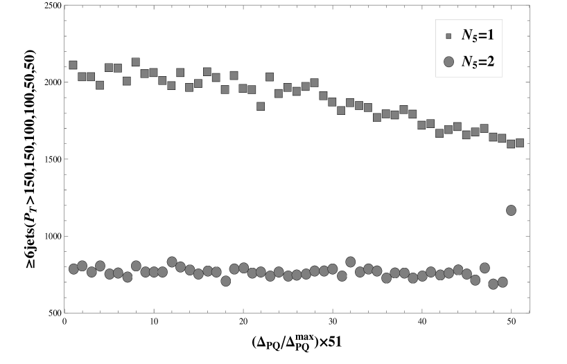
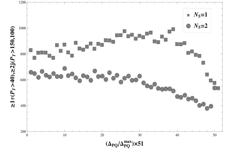
Figure 23: LHC signatures as functions of $\Delta_{PQ}$ for F-theory GUTs with ($N_{5}=1$,$\Lambda=1.2\times 10^{5}$ GeV) and ($N_{5}=2$,$\Lambda=6.5\times 10^{4}$ GeV). The signatures are simulated with $5$ fb^-1 of integrated luminosity. These plots show that the LHC signatures are sensitive to the “stringy” parameter $\Delta_{PQ}$.

Given the prominent role of the PQ deformation in F-theory GUTs, it is important to find signatures sensitive to the value of $\Delta{PQ}$. Because the effects of $\Delta_{PQ}$ are most prominent for bino NLSP F-theory GUTs with a single messenger, we confine our discussion to this case. As explained in section 2, the PQ deformation alters both the masses and branching fractions. A non-zero PQ deformation leads to two major observable effects. First, the charginos produced either directly or from gluino and squark decay will undergo cascade decays of the form $\tilde{\chi}_{1}^{\pm}\rightarrow\tilde{\tau}^{\pm}_{1}\nu_{\tau}\rightarrow\tilde{\chi}_{1}^{0}\tau^{\pm}\nu_{\tau}$. The branching ratio of this channel will increase as $\Delta_{PQ}$ increases, and at the same time, the taus produced from the decay of the $\tilde{\tau}_{1}$ will become less energetic. Based on these changes, our expectation is that signatures related to $\tau$’s or soft jets in the final state will be helpful in distinguishing these models. Second, in comparison to the other squarks, the mass of lightest stop $\tilde{t}_{1}$ is more sensitive to $\Delta_{PQ}$. This leads to changes in the branching ratio of the gluino decay into third generation quarks, which is particularly important in the case of single messenger models. This can be probed by using signatures related to third generation quarks in the final state.

4.2 Determining $N_{5}$ and $\Lambda$

Having established a set of signatures with strong dependence on the parameters of F-theory GUTs, in this section we compute the value of $\Delta S_{(D)}^{2}$ specified by the signatures of table 4 between a given F-theory GUT “LHC point”and all other F-theory GUTs. Minimizing $\Delta S_{(D)}^{2}$ over the class of all F-theory GUTs with a bino NLSP, we can then in principle extract the corresponding values of $N_{5}$ and $\Lambda$. In computing the value of $\Delta S_{(D)}^{2}$ between models with a single messenger, and models with multiple messengers, we find that $\Delta S_{(D)}^{2}$ is typically greater (sometimes far greater) than $10$. Based on this, we conclude that it is typically possible to distinguish single messenger models from multiple messenger models. On the other hand, distinguishing between multiple messenger models appears more challenging. As an explicit example, figure 24 shows the value of $\Delta S_{(D)}^{2}$ between three messenger F-theory models and a two messenger F-theory GUT model with $\Lambda=8\times 10^{4}$ GeV and $\Delta_{PQ}=104$ GeV, which contains a region of models with $\Delta S_{(D)}^{2}<2.3$. Indeed, as explained earlier, the mass spectra are much closer in such cases. Even so, the decay of the gluino is different depending on the number of messengers (for example, see the branching fractions of (30) in subsection 2.5.2). Although beyond the scope of this paper, it would be interesting to study whether signatures sensitive to the decay $\widetilde{g}\rightarrow\widetilde{t}t$ could provide a means to distinguish between two and three messenger F-theory GUTs.

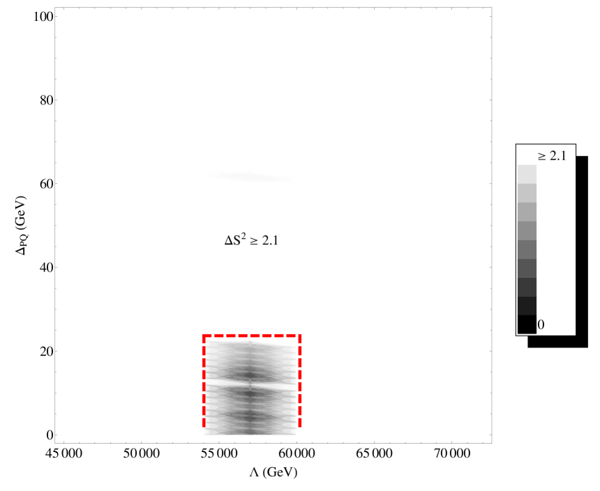
Figure 24: Density plot of $\Delta S_{(D)}^{2}$ defined by the signature list in table 4 of subsection 4.1 between a two messenger F-theory GUT model with $\Lambda=8\times 10^{4}$ GeV and $\Delta_{PQ}=104$ GeV and three messenger F-theory GUTs. Using a rough notion of distinguishability compatible with a chi-square measure, models with $\Delta S_{(D)}^{2}>2.1$ are distinguishable from this “LHC point” at the $99\%$ level for $13$ signals. Note that $\Delta S_{(D)}^{2}$ possesses a local minimum, even though the number of messengers is incorrect. This illustrates that distinguishing $N_{5}=2$ and $N_{5}=3$ is more subtle with limited luminosity.

Nevertheless, this analysis does establish that it is indeed possible to distinguish between single and multiple messenger models. Assuming that the discrete parameter $N_{5}$ has been determined, the largest difference between various models is the value of $\Lambda$. Focussing for simplicity on the case of a single messenger model, we find that the value of $\Delta S_{(D)}^{2}$ minimizes at a single value of $\Lambda$. As an explicit example, figure 25 shows the value of $\Delta S_{(D)}^{2}$ between all single messenger F-theory models and a single messenger F-theory GUT model with $\Lambda=1.44\times 10^{5}$ GeV and $\Delta_{PQ}=164$ GeV. Note in particular that the density plot minimizes at a particular value of $\Lambda$, and that furthermore, there is a lower bound to the value of $\Delta_{PQ}$ in the region where $\Delta S_{(D)}^{2}<2.3$. We therefore conclude that even at $5$ fb^-1, it is possible to distinguish single messenger models from multiple messenger models, and moreover, once the number of messengers has been determined, to extract the value of $\Lambda$, and a crude bound on $\Delta_{PQ}$.

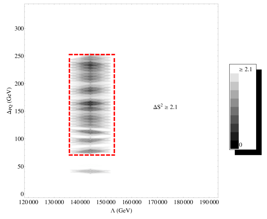
Figure 25: Density plot of $\Delta S_{(D)}^{2}$ defined by the signature list in table 4 of subsection 4.1 between a single messenger F-theory GUT model with $\Lambda=1.44\times 10^{5}$ GeV and $\Delta_{PQ}=164$ GeV and other single messenger F-theory GUTs. Here, we have used a rough notion of distinguishability based on $99\%$ confidence and $13$ signals so that at $\Delta S_{(D)}^{2}>2.3$ we shall say that two models are distinguishable. Note that $\Delta S_{(D)}^{2}$ minimizes near the correct value of $\Lambda$, and that moreover, the value of $\Delta_{PQ}$ can be distinguished as a non-zero value up to $\sim\pm 100$ GeV. The small shaded area just outside the dashed box is absent when SM background is turned off.

4.3 Determining $\Delta_{PQ}$ at $5$ fb^-1 and $50$ fb^-1

To completely distinguish between F-theory GUTs and a generic mGMSB model, we next turn to the determination of $\Delta_{PQ}$. As opposed to the discrete parameter $N_{5}$ and the gaugino mass unification scale $\Lambda$, the dependence of the mass spectrum on the parameter $\Delta_{PQ}$ is somewhat smaller. In particular, in the case of multiple messenger models, the most pronounced effect of the PQ deformation only occurs in a regime of parameter space where the stau is already the NLSP. Since the primary focus of our current analysis is on the more difficult case of a bino NLSP, we shall therefore restrict attention to the single messenger case.

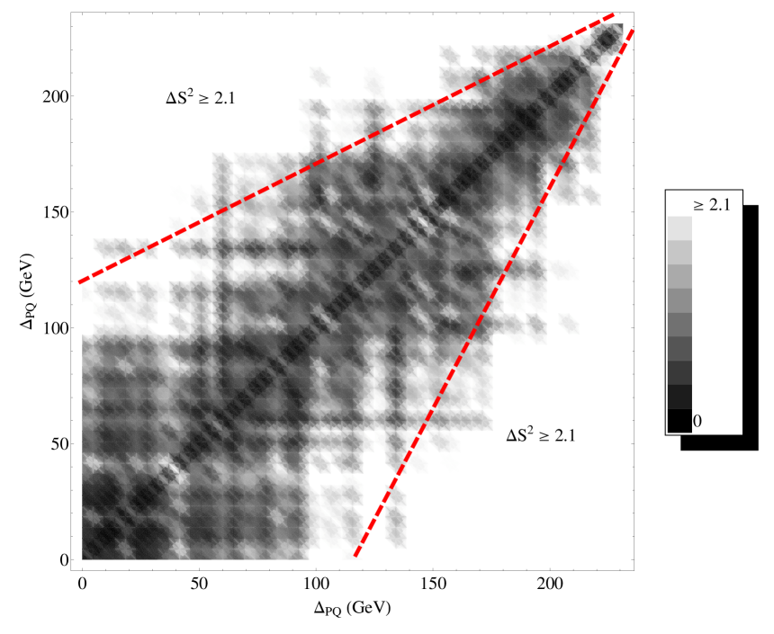
Figure 26: Density plot of $\Delta S_{(D)}^{2}$ defined by the signature list in table 4 of subsection 4.1 at 5 fb^-1 of simulated data comparing F-theory GUTs with $N_{5}=1$ and $\Lambda=1.28\times 10^{5}$ GeV, but with varying values of the PQ deformation parameter. Here, we have used a rough notion of distinguishability based on $99\%$ confidence and $13$ signals so that at $\Delta S_{(D)}^{2}>2.3$ we shall say that two models are distinguishable. This plot illustrates that $\Delta S_{(D)}^{2}$ minimizes in a neighborhood of the region $\Delta^{(1)}_{PQ}=\Delta^{(2)}_{PQ}$. Note in addition that the determination of $\Delta_{PQ}$ becomes more accurate at larger values of the PQ deformation.

In order to determine whether it is possible to extract the value of $\Delta_{PQ}$, we computed the value of $\Delta S_{(D)}^{2}$ between any two F-theory GUT models with the same values for $N_{5}$ and $\Lambda$. As an illustrative example, we considered in detail the case of $N_{5}=1$ and $\Lambda=1.28\times 10^{5}$ GeV. Plotting the value of $\Delta S_{(D)}^{2}$ as a function of the PQ deformation parameter of the two models, $\Delta_{PQ}^{(1)}$ and $\Delta_{PQ}^{(2)}$, we find that at $5$ fb^-1 of simulated data, $\Delta S_{(D)}^{2}$ achieves a minimum over a somewhat broad range of values. See figure 26 for a plot of $\Delta S_{(D)}^{2}$ at $5$ fb^-1 of integrated luminosity. This figure also illustrates that although this range is somewhat broad at low values of $\Delta_{PQ}$, with an error on the order of $\sim\pm 100$ GeV, at larger values of $\Delta_{PQ}$, the region with $\Delta S_{(D)}^{2}<2.1$ occurs over a smaller range of values. We therefore conclude that it is indeed possible to distinguish between models with very low $\Delta_{PQ}$ and very large $\Delta_{PQ}$. Increasing the luminosity allows for further refinements in the determination of $\Delta_{PQ}$. Figure 27 illustrates that as a function of the two PQ deformations, the value of $\Delta S_{(D)}^{2}$ at $50$ fb^-1 allows us to determine the value of $\Delta_{PQ}$ on the order of $\sim\pm 10$ GeV.

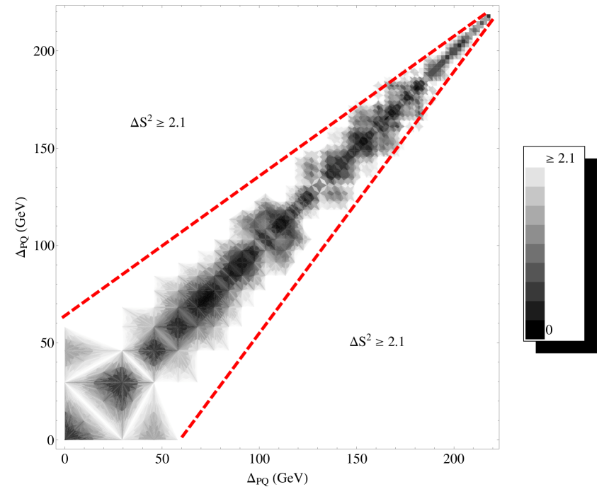
Figure 27: Density plot of $\Delta S_{(D)}^{2}$ defined by the signature list in table 4 of subsection 4.1 at 50 fb^-1 of simulated data comparing F-theory GUTs with $N_{5}=1$ and $\Lambda=1.28\times 10^{5}$ GeV, but with varying values of the PQ deformation parameter. Here, we have used a rough notion of distinguishability based on $99\%$ confidence and $13$ signals so that at $\Delta S_{(D)}^{2}>2.1$ we shall say that two models are distinguishable. This plot illustrates that $\Delta S_{(D)}^{2}$ minimizes in a neighborhood of the region $\Delta^{(1)}_{PQ}=\Delta^{(2)}_{PQ}$. As opposed to the case of 5 fb^-1 of simulated data shown in figure 26, at increased luminosity, it is possible to extract more detailed information about the PQ deformation.

5 Conclusions

In this paper we have analyzed the extent to which with a relatively low integrated luminosity of $5$ fb^-1 how well the LHC can distinguish F-theory GUTs from other scenarios with an MSSM spectrum. Focussing on the case of F-theory GUTs with a bino NLSP, we have used a footprint analysis to determine signatures of potential interest. We have found that collider signatures with multijets plus missing energy, as well as b-jets and taus are typically able to distinguish this scenario from mSUGRA models with small A-terms and from low scale minimal GMSB scenarios. In addition, single messenger F-theory GUTs can be distinguished from mSUGRA models with large A-terms. We have also found that mSUGRA models with large A-terms can potentially mimic the signatures of multiple messenger F-theory GUTs with a bino NLSP. With $5$ fb^-1 of integrated luminosity, we find that these models can only be distinguished from large A-term mSUGRA models in a small range of F-theory GUT parameter space.

Focusing on just F-theory GUTs, we have also examined how well collider signatures can be used to determine the extract the defining parameters of the model, given by the number of messengers $N_{5}$, the characteristic mass scale of minimal gauge mediation $\Lambda$, and the stringy PQ deformation parameter $\Delta_{PQ}$. We have found that it is typically possible to distinguish between single and multiple messenger F-theory GUTs, although due to the similarities in the soft parameters, distinguishing between two and three messenger models appears more challenging. We have also seen that once the number of messengers has been fixed, extracting the value of $\Lambda$ is quite straightforward. More importantly, we have also seen that a distinctively stringy feature of F-theory GUTs corresponding to a deformation away from a minimal gauge mediation scenario has observable consequences. Indeed, with $5$ fb^-1 of integrated luminosity, it is possible to distinguish the value of this parameter up to $\sim\pm 80$ GeV, while for $50$ fb^-1, this distinguishability typically improves to $\sim\pm 10$ GeV.

One of the advantages of the footprint method is that rather than performing a global fit to the data, specifying particular signatures which are sensitive to characteristics of a class of models provides a relatively simple methodology for distinguishing between broad classes of models. Using the footprint as a sieve for various models, we have seen that in tandem with more quantitative measures, it is possible to distinguish F-theory GUTs from other well-motivated models with an MSSM spectrum. On the other hand, it would of course be of interest to analyze a global chi-square fit to a given model by including a large class of binned $P_{T}$ distributions, and other similar observables. Utilizing the entire class of such observables, a given F-theory GUT will define a vector in a very high-dimensional vector space. Performing a fit to such models, it would be important to ascertain the level of resolution expected in parameters such as the PQ deformation.

In this paper we have primarily focussed on signatures obtained which can be obtained from the LHC with low integrated luminosity. Performing a similar study with high luminosity would certainly be very interesting. First, this would allow us to distinguish F-theory GUTs from other models more cleanly, with more available signatures and better statistics. Second, it would also allow us to study the potential for performing mass reconstruction of superpartners. This would provide a more direct verification of the mass spectrum of F-theory GUTs, and would in particular directly probe the effects of the PQ deformation. Of course, for future study, improved signal and background simulation is certainly necessary in order to confront real LHC data.

In addition, while our analysis has primarily focussed on determining a class of signatures which can distinguish F-theory GUTs from other models, our explanation for why these particular signals are effective in discriminating between various models was based on a somewhat heuristic analysis of the spectrum and branching fractions. It would be interesting to perform a more systematic simulation study to determine whether other potentially interesting signatures can be extracted. For example, the angular distribution of electrons and muons (or also the somewhat different case of taus) could potentially provide another window into the physics of F-theory GUTs.

Although we have focussed on the case of F-theory GUTs with a bino NLSP, the case of stau NLSP scenarios is also possible, especially in the case of multiple messenger models. We have focussed on the bino NLSP case because it does not contain as striking a signature as a quasi-stable stau. Nevertheless, it would be interesting to explore in greater detail this regime of F-theory GUTs using the footprint method.

Appendix A: Benchmark mSUGRA Scans

In this Appendix we describe the mSUGRA parameter scan and the mSUGRA models studied in our comparison with F-theory GUTs. We recall that such models are specified by the parameters $M_{1/2}$, $m_{0}$, $A$ and a choice of $\tan\beta$. For simplicity, we have primarily restricted our interest to models where the colored sparticle sector has similar masses to the case of F-theory GUTs. We first describe the scan performed over mSUGRA models with small A-term. We have considered the following range of parameters:

• $M_{1/2}=400-600$

• $m_{0}=M_{1/2}(2.5+\epsilon)$, with $-0.3\lesssim\epsilon\lesssim-0.3$

• $A=0-400$

• $\tan\beta=2-47$.

We note that in the above scan we have correlated the squark mass with the gluino mass, allowing it to have a small amount of variation parameterized by $\epsilon$. In this scan, we have generated $180$ mSUGRA models, which we shall refer to as small A-term mSUGRA models in our comparison with F-theory GUT models.

In the above scan, we have restricted our attention to models with small A-terms. It is also of interest to study mSUGRA models with large A-terms. When the A-term is large, there will be some qualitative differences in the mass spectrum. Most important is the fact that due to the large trilinear couplings, the lightest stau can now have mass in between that of $\tilde{\chi}_{1}^{0}$ and $\tilde{\chi}_{2}^{0}$, much as in F-theory GUTs with a bino NLSP. For this reason, we have also performed a scan over mSUGRA models with large A-term:

• $M_{1/2}=400-600$

• $m_{0}=M_{1/2}(2.5+\epsilon)$, with $-1.5\lesssim\epsilon\lesssim 0.5$

• $A=0-3000$

• $\tan\beta=2-50$,

We have generated a total of $13728$ such models, of which $255$ models satisfy the stau mass condition $m_{\tilde{\chi}_{1}^{0}}<m_{\tilde{\tau}_{1}}<m_{\tilde{\chi}_{2}^{0}}$ and the Higgs mass limit $m_{h}>114$ GeV. Both of these conditions significantly constrain the allowed parameter space. This subset of mSUGRA models are referred to as the large A-term mSUGRA models in our comparison with F-theory GUT models.

Appendix B: Benchmark Low Scale mGMSB With Stau NLSP Scans

For the low scale mGMSB models, we focus on the case with $\tilde{\tau}$ NLSP. In this case, the lightest stau will decay inside the detector giving rise to missing $E_{T}$ signatures. Because of the generic presence of taus in the events, this class of models can in principal mimic F-theory GUTs with a missing $E_{T}$ signal, corresponding to the case of F-theory GUTs with a bino NLSP.

In this Appendix we describe the scan over low messenger scale mGMSB models we have performed. To generate a scan of such models, we vary the parameters $N_{5}$, $\Lambda$, $\tan\beta$ of mGMSB scenarios. For simplicity, we fix the messenger scale $M_{\text{mess}}$ to a low energy scale, since it only changes the sparticle mass spectrum logarithmically. The scan we have performed comprises the following range of parameters:

• $N_{5}=1$

  • $M_{\text{mess}}=2\times 10^{5}$ GeV

  • $\Lambda=(1.2-1.92)\times 10^{5}$ GeV with step size $8\times 10^{3}$ GeV

• $N_{5}=2$

  • $M_{\text{mess}}=1.2\times 10^{5}$ GeV

  • $\Lambda=(6.5-11)\times 10^{4}$ GeV with step size $5\times 10^{3}$ GeV

• $N_{5}=3$

  • $M_{\text{mess}}=1.2\times 10^{5}$ GeV

  • $\Lambda=(4.5-7.2)\times 10^{4}$ GeV with step size $3\times 10^{3}$ GeV

• for all of these cases, $\tan\beta\sim 2-50$ with step size $2$.

In the above scan, the lower limit on $\Lambda$ corresponds to the Higgs mass bound $m_{h}>114$ GeV, and the upper limit corresponds to the discovery limit for $5$ fb^-1. Of the $750$ low scale mGMSB models generated this way, $433$ of these have a stau NLSP.

Appendix C: Signature List

In this Appendix we provide a list of the 103 signatures used in our footprint analysis. Most of the signatures are based on the inclusive $2$ jet and $4$ jet plus missing $E_{T}$ selections as listed in table 1 of subsection 3.1. The counts of events of these two selections are denoted by $\geq 2$jets($P_{T}>150,100$) and $\geq 4$jet($P_{T}>100,50,50,50$) respectively. These two selections are further divided into subsets according to the number of leptons, taus and b-jets. The selection criteria are given below:

• leptons: $0l$, $\geq 1l$, $\geq 2l$, opposite-sign $2l$ (OSDL) and same-sign $2l$ (SSDL).

• taus: $0\tau$, $\geq 1\tau$, $\geq 2\tau$, opposite-sign $2\tau$ (OSDT) and same-sign $2\tau$ (SSDT).

• b-jets: $0b$, $\geq 1b$, $\geq 2b$ and $\geq 3b$

• leptons + b-jets: $0l0b$, $0l\geq 1b$, $0l\geq 2b$, $\geq 1l0b$, $\geq 1l\geq 1b$, $\geq 1l\geq 2b$, $\geq 2l0b$

• taus + b-jets: $0\tau 0b$, $0\tau\geq 1b$, $0\tau\geq 2b$, $\geq 1\tau 0b$, $\geq 1\tau\geq 1b$, $\geq 1\tau\geq 2b$, $\geq 2\tau 0b$

• where we used two different $P_{T}$ cuts for each object:

  • $P_{T}>10$,$40$ GeV for lepton and tau

  • $P_{T}>50$,$100$ GeV for b-jet.

Additional signatures include some variations of the selection criteria (if not specified ${\displaystyle}{\not}E_{T}>100$ GeV and $M_{eff}>1200$), which are listed below:

• $\geq 6$ jets ($P_{T}>100,100,20,20,20,20$), ${\displaystyle}{\not}E_{T}>200$ GeV

• $\geq 6$ jets ($P_{T}>100,100,100,100,20,20$)

• $\geq 1\tau$($P_{T}>40$), $\geq 2$jets($P_{T}>80$)

• $\geq 1\tau$($P_{T}>40$), $\geq 4$jets($P_{T}>40$)

• $\geq 1\tau$($P_{T}<40$), $\geq 4$jets($P_{T}>40$), ${\displaystyle}{\not}E_{T}>150$ GeV

• $\geq 1\tau$($P_{T}<40$), $\geq 4$jets($P_{T}>40$), ${\displaystyle}{\not}E_{T}>150$ GeV

• $\geq 2$jets($P_{T}>350$), ${\displaystyle}{\not}E_{T}>0.2M_{eff}$

• $\geq 4$jets($P_{T}>250,250,150,150$), ${\displaystyle}{\not}E_{T}>0.1M_{eff}$

• $\geq 6$jets($P_{T}>150,150,100,100,50,50$)

The last set of signatures are based on [42], where the base cut is given by ${\displaystyle}{\not}E_{T}>150$ GeV and $M_{eff}>600$ GeV.

• $0l$($P_{T}>20$),$\leq 4$jets($P_{T}>50$), $E_{T}^{miss}>500$ GeV

• $0l$($P_{T}>20$),$\leq 4$jets($P_{T}>50$), $M_{eff}>1500$ GeV

• $\geq 1l$($P_{T}>20$), $\leq 4$jets($P_{T}>50$), ${\displaystyle}{\not}E_{T}>0.2M_{eff}$ and $M_{eff}>1400$ GeV

• $0l$($P_{T}>20$),$\geq 5$jets($P_{T}>50$), $M_{eff}>1200$ GeV

• $0l$($P_{T}>20$),$\geq 5$jets($P_{T}>50$), 4th hardest jet $P_{T}>100$ GeV

• $0l$($P_{T}>20$),$\geq 5$jets($P_{T}>50$), $0.15<r_{\rm jet}<0.5$

• $0l$($P_{T}>20$),$\geq 5$jets($P_{T}>50$), $0.5<r_{\rm jet}<1.0$

• $0l$($P_{T}>20$),$\geq 5$jets($P_{T}>50$), $0.05<E_{T}^{miss}/M_{eff}<0.35$

• $\geq 1l$($P_{T}>20$),$\geq 5$jets($P_{T}>50$), $M_{eff}>1350$ GeV

• $\geq 1l$($P_{T}>20$),$\geq 5$jets($P_{T}>50$), 4th hardest jet $P_{T}>100$ GeV

• $\geq 1l$($P_{T}>20$),$\geq 5$jets($P_{T}>50$), hardest lepton $P_{T}>60$ GeV

• $\geq 1l$($P_{T}>20$),$\geq 5$jets($P_{T}>50$), $0.05<{\displaystyle}{\not}E_{T}/M_{eff}<0.35$

• $\geq 1\tau$($P_{T}>20$),$\geq 5$jets($P_{T}>50$), $M_{eff}>1350$ GeV

• $\geq 1\tau$($P_{T}>20$),$\geq 5$jets($P_{T}>50$), 4th hardest jet $P_{T}>100$ GeV

• $\geq 1\tau$($P_{T}>20$),$\geq 5$jets($P_{T}>50$), hardest tau $P_{T}>60$ GeV

• $\geq 1\tau$($P_{T}>20$),$\geq 5$jets($P_{T}>50$), $0.05<{\displaystyle}{\not}E_{T}/M_{eff}<0.35$

For all $103$ signatures, we have imposed the cut on transverse sphericity $S_{T}>0.2$. In the above signature, the value $r_{\rm jet}$ is given as a function of the jet $P_{T}$’s as:

$$r_{\rm jet}\equiv\frac{P_{T}^{\rm jet3}+P_{T}^{\rm jet4}}{P_{T}^{\rm jet1}+P_{T}^{\rm jet2}},$$ (60)

where $P_{T}^{{\rm jet}i}$ is the transverse momentum of the $i$-th hardest jet in the event. For this signature we require at least three jets with $P_{T}>200$ GeV.

Appendix D: PGS Trigger

In our simulation, we have used the PGS4 default detector configuration and cone jet algorithm with a cone size $0.5$. In addition, the PGS loose b-tagging is used, which corresponds to a tagging probability near $0.5$ in the central region for high energy jets. To reduce the number of SM background events, we choose the PGS triggers with high thresholds:

• Inclusive isolated lepton ($e$,$\mu$) $180$ GeV

• Lepton plus jet ($130$ GeV, $200$ GeV)

• Isolated dileptons ($\mu\mu$,$ee$) $60$ GeV

• Dileptons($\mu\mu$,$ee$) plus jet ($45$ GeV, $150$ GeV)

• Isolated dileptons ($e\mu$) $30$ GeV

• Isolated lepton ($\mu$,$e$) plus isolated tau ($45$ GeV, $60$ GeV)

• Isolated ditau $60$ GeV

• Inclusive isolated photon $80$ GeV

• Isolated diphoton $40$ GeV

• Inclusive ${\displaystyle{\not}E_{T}}$ $200$ GeV

• Inclusive single-jet $1000$ GeV

• Jet plus ${\displaystyle{\not}E_{T}}$ ($300$ GeV, $125$ GeV)

• Accoplanar jet and ${\displaystyle{\not}E_{T}}$ ($150$ GeV, $80$ GeV, $1<\Delta\phi<2$)

• Accoplanar dijets ($400$ GeV, $\Delta\phi<2$)

Appendix E: PQ deformation and Ditau Mass Distribution

In this Appendix we present a general discussion of the prospects of using the ditau mass distribution as an additional means of probing the PQ deformation in F-theory GUTs with a bino NLSP. We find that for given $N_{5}$ and $\Lambda$, the edge of the ditau mass distribution is sensitive to the PQ deformation. Interestingly, for F-theory GUTs with $N_{5}=2,3$, measuring the edge of the ditau mass distribution will uniquely determine the PQ deformation. For the case with $N_{5}=1$, the PQ deformation can be determined up to a two-fold degeneracy.

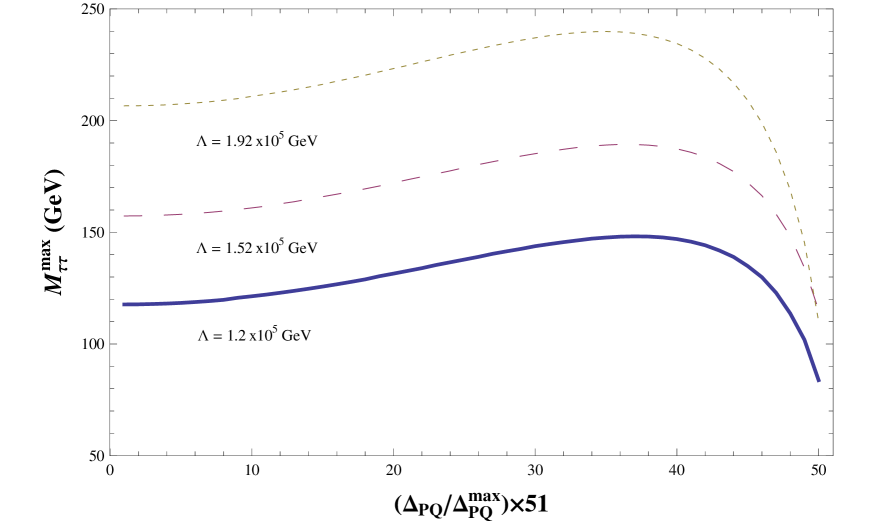
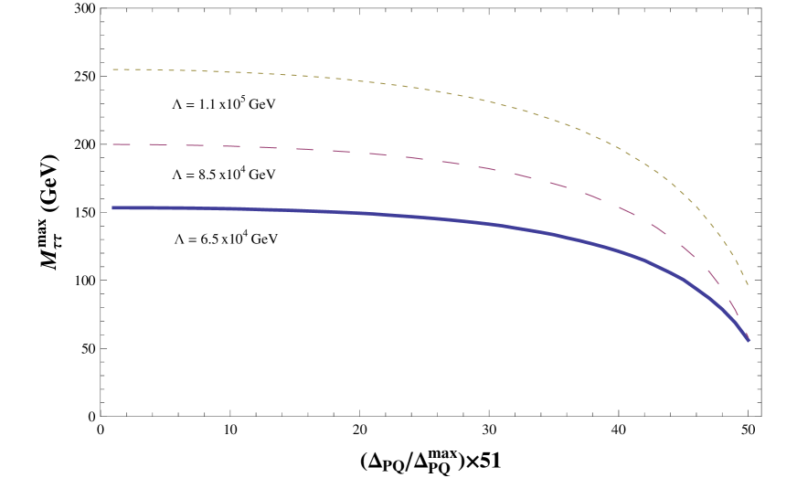
Figure 28: Endpoint of the opposite-sign ditau invariant mass distribution as a function of the PQ deformation parameter $\Delta_{PQ}$ for F-theory GUTs with a bino NLSP. From top to bottom, the two plots are for $N_{5}=1,2$ respectively. The case of $N_{5}=3$ is similar to $N_{5}=2$. Note that in contrast to the case of a single messenger model, for two and three messengers, the endpoint decreases monotonically as a function of $\Delta_{PQ}$.

When the bino is the NLSP, the relative masses of the lightest stau and two lightest neutralinos obey the relation:

$$m_{\widetilde{\chi}_{1}^{(0)}}<m_{\widetilde{\tau}_{1}}<m_{\widetilde{\chi}_{2}^{(0)}}\text{.}$$ (61)

In this case, the decay chain:

$$\widetilde{\chi}_{2}^{(0)}\rightarrow\widetilde{\tau}_{1}^{\pm}\tau^{\mp}\rightarrow\widetilde{\chi}_{1}^{(0)}\tau^{\pm}\tau^{\mp}$$ (62)

will generate events with opposite sign taus. If the $\tau^{+}\tau^{-}$ mass distribution could be measured directly, it would show a sharp kinematical edge

$$(m_{\tau^{+}\tau^{-}}^{\max})^{2}\equiv\frac{\left(m_{\widetilde{\chi}_{2}^{(0)}}^{2}-m_{\widetilde{\tau}_{1}}^{2}\right)\left(m_{\widetilde{\tau}_{1}}^{2}-m_{\widetilde{\chi}_{1}^{(0)}}^{2}\right)}{m_{\widetilde{\tau}_{1}}^{2}}\text{.}$$ (63)

However in practice, this edge structure gets smeared out by the missing neutrino from the tau decay. In addition, there will be a large background under the edge due to the fake taus from jets as well as taus from the chargino decay $\chi_{1}^{\pm}\rightarrow\tilde{\tau}^{\pm}\nu$. In spite of these potential complications, this edge can be experimentally measured with an estimated $10\%$ error for a few tens of fb^-1 integrated luminosity [40].

With this in mind, we now show that the endpoint of the ditau invariant mass distribution is is sensitive to the PQ deformation. Scanning over models with different values of $\Delta_{PQ}$, figure 28 shows that $m_{\tau^{+}\tau^{-}}^{\max}$ is a non-trivial function of $\Delta_{PQ}$. Since the parameter $\Lambda$ and $N_{5}$ are relatively easy to determine, we shall take them as fixed in the following discussion. For the one messenger case, there is one-to-one correspondence between the $m_{\tau^{+}\tau^{-}}^{\max}$ and $\Delta_{PQ}$ in the very large $\Delta_{PQ}$ region, but generally shows a two-fold degeneracy between small and large $\Delta_{PQ}$. In this case, the value of $m_{\tau^{+}\tau^{-}}^{\max}$ cannot by itself be used to determine the PQ deformation, and requires supplementary observables, such as $P_{T}$ distributions, to the resolve the degeneracy. However, for the two and three messenger cases, there is always a one-to-one correspondence between the value of $m_{\tau^{+}\tau^{-}}^{\max}$ and $\Delta_{PQ}$. This makes the ditau invariant mass edge an effective observable for probing the PQ deformation in F-theory GUTs.

In the following, we shall not focus on the concrete extraction of the ditau invariant mass edge from the simulated data. Instead, we focus on the analytic dependence of $m_{\tau^{+}\tau^{-}}^{\max}$ on $\Delta_{PQ}$. As a rough approximation, the PQ deformation can simply be added as an overall shift to $m_{\widetilde{\tau}_{1}}$. Letting $\widehat{m}_{\widetilde{\tau}_{1}}$ denote the lightest stau mass in the absence of the PQ deformation, the endpoint of the ditau invariant mass distribution is given by the approximation:

$$(m_{\tau^{+}\tau^{-}}^{\max})^{2} \sim\frac{\left(m_{\widetilde{\chi}_{2}^{(0)}}^{2}-\widehat{m}_{\widetilde{\tau}_{1}}^{2}+\Delta_{PQ}^{2}\right)\left(\widehat{m}_{\widetilde{\tau}_{1}}^{2}-\Delta_{PQ}^{2}-m_{\widetilde{\chi}_{1}^{(0)}}^{2}\right)}{\widehat{m}_{\widetilde{\tau}_{1}}^{2}-\Delta_{PQ}^{2}}$$ (64)

$$=m_{\widetilde{\chi}_{2}^{(0)}}^{2}+m_{\widetilde{\chi}_{1}^{(0)}}^{2}-\frac{m_{\widetilde{\chi}_{2}^{(0)}}^{2}m_{\widetilde{\chi}_{1}^{(0)}}^{2}}{\widehat{m}_{\widetilde{\tau}_{1}}^{2}-\Delta_{PQ}^{2}}-\left(\widehat{m}_{\widetilde{\tau}_{1}}^{2}-\Delta_{PQ}^{2}\right)$$ (65)

$$=\widehat{m}_{\widetilde{\tau}_{1}}^{2}\left(A-\frac{B}{1-x}-(1-x)\right)$$ (66)

where we have introduced the parameters:

$$A \equiv\frac{m_{\widetilde{\chi}_{2}^{(0)}}^{2}+m_{\widetilde{\chi}_{1}^{(0)}}^{2}}{\widehat{m}_{\widetilde{\tau}_{1}}^{2}}$$ (67)

$$B \equiv\frac{m_{\widetilde{\chi}_{2}^{(0)}}^{2}m_{\widetilde{\chi}_{1}^{(0)}}^{2}}{\widehat{m}_{\widetilde{\tau}_{1}}^{4}}$$ (68)

$$x \equiv\frac{\Delta_{PQ}^{2}}{\widehat{m}_{\widetilde{\tau}_{1}}^{2}}\text{.}$$ (69)

We now determine the behavior of $(m_{\tau^{+}\tau^{-}}^{\max})^{2}$ as a function of $x$ as $x$ ranges from zero ($\Delta_{PQ}=0$) to 1 ($\Delta_{PQ}=\widehat{m}_{\widetilde{\tau}_{1}}$). To this end, we now show that depending on the initial placement of the lightest stau mass, the value of $(m_{\tau^{+}\tau^{-}}^{\max})^{2}$ can either increase, or decrease. Note, however, that at $x=1$, the value of $(m_{\tau^{+}\tau^{-}}^{\max})^{2}$ vanishes. The value of $(m_{\tau^{+}\tau^{-}}^{\max})^{2}$ will increase provided a local maximum is present between $x=0$ and $x=1$. The function $(m_{\tau^{+}\tau^{-}}^{\max})^{2}(x)$ possesses a critical point satisfying the condition:

$$x_{\ast}=1-\sqrt{B}=1-\frac{m_{\widetilde{\chi}_{2}^{(0)}}m_{\widetilde{\chi}_{1}^{(0)}}}{\widehat{m}_{\widetilde{\tau}_{1}}^{2}}\text{.}$$ (70)

Computing the second derivative of $(m_{\tau^{+}\tau^{-}}^{\max})^{2}(x)$ with respect to $x$, it follows that this corresponds to a local maximum for the function. In other words, for $x<x_{\ast}$, $(m_{\tau^{+}\tau^{-}}^{\max})^{2}(x)$ increases, while for $x>x_{\ast}$, $(m_{\tau^{+}\tau^{-}}^{\max})^{2}(x)$ decreases.

This local maximum will only be attained in the physical range of interest when $0<x_{\ast}<1$, or:

$$0<\widehat{m}_{\widetilde{\tau}_{1}}^{2}-m_{\widetilde{\chi}_{2}^{(0)}}m_{\widetilde{\chi}_{1}^{(0)}}<\widehat{m}_{\widetilde{\tau}_{1}}^{2}\text{.}$$ (71)

While the second inequality is indeed always satisfied, the first inequality requires the geometric mean of $m_{\widetilde{\chi}_{2}^{(0)}}$ and $m_{\widetilde{\chi}_{1}^{(0)}}$ to be less than $\widehat{m}_{\widetilde{\tau}_{1}}$. When this inequality is not satisfied so that $x_{\ast}<0$, it follows that $(m_{\tau^{+}\tau^{-}}^{\max})^{2}(x)$ is always a decreasing function over the physically acceptable range of values for $\Delta_{PQ}$. In the case where a local maximum is achieved, there is a potential degeneracy in the location of the endpoint. For large enough values of the PQ deformation, however, there is typically no degeneracy because there is a single local maximum and the endpoint must vanish at the point where the stau and bino masses become degenerate. See figure 28 for plots of the endpoint for representative F-theory GUTs with $N_{5}=1,3$ vector-like pairs of messengers. These plots illustrate that the relative spacing between the lightest stau and the two lightest neutralinos can produce qualitatively different $\Delta_{PQ}$ dependence.

Appendix F: Miscellaneous Plots

In this Appendix we collect additional plots of potential interest.

References

- [1] C. Beasley, J. J. Heckman, and C. Vafa, “GUTs and Exceptional Branes in F-theory - II: Experimental Predictions,” JHEP 01 (2009) 059, arXiv:0806.0102 [hep-th].
- [2] C. Beasley, J. J. Heckman, and C. Vafa, “GUTs and Exceptional Branes in F-theory - I,” JHEP 01 (2009) 058, arXiv:0802.3391 [hep-th].
- [3] J. J. Heckman, J. Marsano, N. Saulina, S. Schäfer-Nameki, and C. Vafa, “Instantons and SUSY breaking in F-theory,” arXiv:0808.1286 [hep-th].
- [4] J. J. Heckman and C. Vafa, “F-theory, GUTs, and the Weak Scale,” arXiv:0809.1098 [hep-th].
- [5] J. J. Heckman and C. Vafa, “From F-theory GUTs to the LHC,” arXiv:0809.3452 [hep-ph].
- [6] J. J. Heckman and C. Vafa, “Flavor Hierarchy From F-theory,” arXiv:0811.2417 [hep-th].
- [7] J. J. Heckman, A. Tavanfar, and C. Vafa, “Cosmology of F-theory GUTs,” arXiv:0812.3155 [hep-th].
- [8] R. Donagi and M. Wijnholt, “Model Building with F-Theory,” arXiv:0802.2969 [hep-th].
- [9] H. Hayashi, R. Tatar, Y. Toda, T. Watari, and M. Yamazaki, “New Aspects of Heterotic–F Theory Duality,” arXiv:0805.1057 [hep-th].
- [10] R. Donagi and M. Wijnholt, “Breaking GUT Groups in F-Theory,” arXiv:0808.2223 [hep-th].
- [11] J. Marsano, N. Saulina, and S. Schäfer-Nameki, “Gauge Mediation in F-Theory GUT Models,” arXiv:0808.1571 [hep-th].
- [12] J. Marsano, N. Saulina, and S. Schäfer-Nameki, “An Instanton Toolbox for F-Theory Model Building,” arXiv:0808.2450 [hep-th].
- [13] M. Wijnholt, “F-Theory, GUTs and Chiral Matter,” arXiv:0809.3878 [hep-th].
- [14] A. Font and L. E. Ibáñez, “Yukawa Structure from U(1) Fluxes in F-theory Grand Unification,” arXiv:0811.2157 [hep-th].
- [15] R. Blumenhagen, V. Braun, T. W. Grimm, and T. Weigand, “GUTs in Type IIB Orientifold Compactifications,” arXiv:0811.2936 [hep-th].
- [16] R. Blumenhagen, “Gauge Coupling Unification in F-theory GUT Models,” arXiv:0812.0248 [hep-th].
- [17] J. L. Bourjaily, “Local Models in F-Theory and M-Theory with Three Generations,” arXiv:0901.3785 [hep-th].
- [18] H. Hayashi, T. Kawano, R. Tatar, and T. Watari, “Codimension-3 Singularities and Yukawa Couplings in F-theory,” arXiv:0901.4941 [hep-th].
- [19] B. Andreas and G. Curio, “From Local to Global in F-Theory Model Building,” arXiv:0902.4143 [hep-th].
- [20] C.-M. Chen and Y.-C. Chung, “A Note on Local GUT Models in F-Theory,” arXiv:0903.3009 [hep-th].
- [21] G. L. Kane, P. Kumar, and J. Shao, “LHC String Phenomenology,” J. Phys. G34 (2007) 1993–2036, hep-ph/0610038.
- [22] G. L. Kane, P. Kumar, and J. Shao, “Unravelling Strings at the LHC,” Phys. Rev. D77 (2008) 116005, arXiv:0709.4259 [hep-ph].
- [23] M. Ibe and R. Kitano, “Sweet Spot Supersymmetry,” JHEP 08 (2007) 016, arXiv:0705.3686 [hep-ph].
- [24] S. P. Martin and J. D. Wells, “Cornering gauge-mediated supersymmetry breaking with quasi-stable sleptons at the Tevatron,” Phys. Rev. D59 (1999) 035008, hep-ph/9805289.
- [25] J. L. Feng and T. Moroi, “Tevatron Signatures of Long-lived Charged Sleptons in Gauge- Mediated Supersymmetry Breaking Models,” Phys. Rev. D58 (1998) 035001, hep-ph/9712499.
- [26] S. Ambrosanio et. al., “SUSY Long-Lived Massive Particles: Detection and Physics at the LHC,” hep-ph/0012192.
- [27] J. R. Ellis, A. R. Raklev, and O. K. Oye, “Gravitino Dark Matter Scenarios with Massive Metastable Charged Sparticles at the LHC,” JHEP 10 (2006) 061, hep-ph/0607261.
- [28] B. C. Allanach, “SOFTSUSY2.0: a program for calculating supersymmetric spectra,” Comput. Phys. Commun. 143 (2002) 305–331, hep-ph/0104145.
- [29] G. F. Giudice and R. Rattazzi, “Theories with Gauge-Mediated Supersymmetry Breaking,” Phys. Rept. 322 (1999) 419–499, hep-ph/9801271.
- [30] T. Sjöstrand, S. Mrenna, and P. Skands, “PYTHIA 6.4 Physics and Manual,” JHEP 05 (2006) 026, hep-ph/0603175.
- [31] M. Muhlleitner, A. Djouadi, and Y. Mambrini, “SDECAY: A Fortran code for the decays of the supersymmetric particles in the MSSM,” Comput. Phys. Commun. 168 (2005) 46–70, hep-ph/0311167.
- [32] B. S. Acharya et. al., “Identifying Multi-Top Events from Gluino Decay at the LHC,” arXiv:0901.3367 [hep-ph].
- [33] B. S. Acharya, K. Bobkov, G. L. Kane, J. Shao, and P. Kumar, “The -MSSM - An Theory motivated model of Particle Physics,” Phys. Rev. D78 (2008) 065038, arXiv:0801.0478 [hep-ph].
- [34] L.-T. Wang and I. Yavin, “A Review of Spin Determination at the LHC,” Int. J. Mod. Phys. A23 (2008) 4647–4668, arXiv:0802.2726 [hep-ph].
- [35] G. L. Kane, A. A. Petrov, J. Shao, and L.-T. Wang, “Initial determination of the spins of the gluino and squarks at LHC,” arXiv:0805.1397 [hep-ph].
- [36] J. Hubisz, J. Lykken, M. Pierini, and M. Spiropulu, “Missing energy look-alikes with 100 pb-1 at the LHC,” Phys. Rev. D78 (2008) 075008, arXiv:0805.2398 [hep-ph].
- [37] M. Burns, K. Kong, K. T. Matchev, and M. Park, “A General Method for Model-Independent Measurements of Particle Spins, Couplings and Mixing Angles in Cascade Decays with Missing Energy at Hadron Colliders,” JHEP 10 (2008) 081, arXiv:0808.2472 [hep-ph].
- [38] O. Gedalia, S. J. Lee, and G. Perez, “Spin Determination via Third Generation Cascade Decays,” arXiv:0901.4438 [hep-ph].
- [39] “PGS, Simple simulation package for generic collider detectors: http://www.physics.ucdavis.edu/conway/research/software/pgs/pgs.html,”.
- [40] The ATLAS Collaboration, G. Aad et. al., “Expected Performance of the ATLAS Experiment - Detector, Trigger and Physics,” arXiv:0901.0512 [hep-ex].
- [41] CMS Collaboration, G. L. Bayatian et. al., “CMS technical design report, volume II: Physics performance,” J. Phys. G34 (2007) 995–1579.
- [42] B. Altunkaynak, P. Grajek, M. Holmes, G. Kane, and B. D. Nelson, “Studying Gaugino Mass Unification at the LHC,” arXiv:0901.1145 [hep-ph].
- [43] N. Arkani-Hamed, G. L. Kane, J. Thaler, and L.-T. Wang, “Supersymmetry and the LHC Inverse Problem,” JHEP 08 (2006) 070, hep-ph/0512190.
- [44] M. Carena, A. Menon, and C. E. M. Wagner, “Minimal Flavor Violation and the Scale of Supersymmetry Breaking,” arXiv:0812.3594 [hep-ph].