The Time-Dependent Schrödinger Equation,
Riccati Equation and Airy Functions

Abstract.

We construct the Green functions (or Feynman’s propagators) for the Schrödinger equations of the form $i\psi_{t}+\frac{1}{4}\psi_{xx}\pm tx^{2}\psi=0$ in terms of Airy functions and solve the Cauchy initial value problem in the coordinate and momentum representations. Particular solutions of the corresponding nonlinear Schrödinger equations with variable coefficients are also found. A special case of the quantum parametric oscillator is studied in detail first. The Green function is explicitly given in terms of Airy functions and the corresponding transition amplitudes are found in terms of a hypergeometric function. The general case of quantum parametric oscillator is considered then in a similar fashion. A group theoretical meaning of the transition amplitudes and their relation with Bargmann’s functions is established.

1. Introduction

In this paper we discuss explicit solutions of the Cauchy initial value problem for the one-dimensional Schrödinger equations

$$i\frac{\partial\psi}{\partial t}+\frac{1}{4}\frac{\partial^{2}\psi}{\partial x^{2}}\pm tx^{2}\psi=0,\qquad\psi\left(x,0\right)=\varphi\left(x\right)$$ (1.1)

with a suitable initial data on the entire real line $\boldsymbol{R}.$ The corresponding Green functions are found in terms of compositions of elementary and Airy functions in the coordinate and momentum representations. It is well-known that the Airy equation describes motion of a quantum particle in the neighborhood of the turning point on the basis of the stationary, or time-independent, Schrödinger equation [15], [38], [73], [41], and [49]. Here we consider an application of these functions to the time-dependent Schrödinger equations for certain parametric oscillator.

It is worth noting that the Green functions for the Schrödinger equation are known explicitly only in a few special cases. An important example of this source is the forced harmonic oscillator originally considered by Richard Feynman in his path integrals approach to the nonrelativistic quantum mechanics [26], [27], [28], [29], and [30]; see also [43]. Since then this problem and its special and limiting cases were discussed by many authors; see Refs. [13], [33], [36], [46], [49], [70] for the simple harmonic oscillator and Refs. [8], [16], [35], [51], [59] for the particle in a constant external field and references therein.

The case of Schrödinger equation with a general variable quadratic Hamiltonian is investigated in Ref. [20]; see also [21], [22], [43], [48], [62], and [63]. Here we present a few examples that are integrable in terms of Airy functions. In this approach, all known exactly solvable quadratic models are classified in terms of solutions of a certain characterization equation. These exactly solvable cases may be of interest in a general treatment of the linear and nonlinear evolution equations; see [12], [17], [18], [19], [39], [42], [47], [64], [69] and references therein. Moreover, these explicit solutions can also be useful when testing numerical methods of solving the time-dependent Schrödinger equations with variable coefficients. The solution of the quantum parametric oscillator problem found in this paper is also relevant.

2. Green Function: Increasing Case

The fundamental solution of the time-dependent Schrödinger equation

$$i\frac{\partial\psi}{\partial t}+\frac{1}{4}\frac{\partial^{2}\psi}{\partial x^{2}}+tx^{2}\psi=0$$ (2.1)

can be found by a familiar substitution [20]

$$\psi=A\left(t\right)e^{iS\left(x,y,t\right)}=\frac{1}{\sqrt{2\pi i\mu\left(t\right)}}e^{i\left(\alpha\left(t\right)x^{2}+\beta\left(t\right)xy+\gamma\left(t\right)y^{2}\right)}.$$ (2.2)

The real-valued functions of time $\alpha\left(t\right),$ $\beta\left(t\right),$ $\gamma\left(t\right)$ satisfy the following system of ordinary differential equations

$$\frac{d\alpha}{dt}-t+\alpha^{2}=0,$$ (2.3)

$$\frac{d\beta}{dt}+\alpha\beta=0,$$ (2.4)

$$\frac{d\gamma}{dt}+\frac{1}{4}\beta^{2}=0,$$ (2.5)

where the first equation is the special Riccati nonlinear differential equation; see, for example, [32], [34], [50], [57], [58], [72] and references therein.

The substitution

$$\alpha=\frac{\mu^{\prime}}{\mu},\qquad\alpha^{\prime}=\frac{\mu^{\prime\prime}}{\mu}-\left(\frac{\mu^{\prime}}{\mu}\right)^{2},$$ (2.6)

which according to Ref. [50] goes back to Jean le Round d’Alembert [23], results in the second order linear equation

$$\mu^{\prime\prime}-t\mu=0.$$ (2.7)

The initial conditions for the corresponding Green function are $\mu\left(0\right)=0$ and $\mu^{\prime}\left(0\right)=1/2.$ It is well-known that Eq. (2.7) can be solved in terms of Airy functions which are studied in detail; see, for example, [1], [3], [50], [53], [67], [72] and references therein. A different definition of these functions that is convenient for our purposes in this paper is given in the Appendix A.

We choose $\mu_{0}=\left(1/2\right)a\left(t\right)$ and the required Green function solution of the system is given by

$$\alpha_{0}=\frac{a^{\prime}\left(t\right)}{a\left(t\right)},\qquad\beta_{0}=-\frac{2}{a\left(t\right)},\qquad\gamma_{0}=\frac{b\left(t\right)}{a\left(t\right)},$$ (2.8)

where the Airy functions $a\left(t\right)=ai\left(t\right)$ and $b\left(t\right)=bi\left(t\right)$ are defined by (12) and (12), respectively. Indeed,

$$\frac{d\beta_{0}}{dt}=-2\left(a^{-1}\right)^{\prime}=2\frac{a^{\prime}}{a^{2}}=-\alpha_{0}\beta_{0},$$ (2.9)

and

$$\frac{d\gamma_{0}}{dt}=\left(\frac{b}{a}\right)^{\prime}=\frac{b^{\prime}a-ba^{\prime}}{a^{2}}=\frac{W\left(a,b\right)}{a^{2}}=-\frac{1}{4}\beta_{0}^{2}.$$ (2.10)

Thus, the Green function has the following closed form

$$G\left(x,y,t\right)=\frac{1}{\sqrt{\pi ia\left(t\right)}}\exp\left(i\frac{a^{\prime}\left(t\right)x^{2}-2xy+b\left(t\right)y^{2}}{a\left(t\right)}\right),\qquad t>0$$ (2.11)

in terms of elementary and Airy functions.

It is worth noting that a more general particular solution has the form

$$\psi=K\left(x,y,t\right)=\frac{1}{\sqrt{2\pi i\mu\left(t\right)}}\ e^{i\left(\alpha\left(t\right)x^{2}+\beta\left(t\right)xy+\gamma\left(t\right)y^{2}\right)},$$ (2.12)

where $\mu=c_{1}a\left(t\right)+c_{2}b\left(t\right)$ with $\mu\left(0\right)=c_{2}\neq 0,$ $\mu^{\prime}\left(0\right)=c_{1}$ and

$$\alpha=\frac{c_{1}a^{\prime}\left(t\right)+c_{2}b^{\prime}\left(t\right)}{c_{1}a\left(t\right)+c_{2}b\left(t\right)},\qquad\alpha\left(0\right)=\frac{c_{1}}{c_{2}},$$ (2.13)

$$\beta=\frac{c_{2}\beta\left(0\right)}{c_{1}a\left(t\right)+c_{2}b\left(t\right)},$$ (2.14)

$$\gamma=\gamma\left(0\right)-\frac{c_{2}\beta^{2}\left(0\right)a\left(t\right)}{4\left(c_{1}a\left(t\right)+c_{2}b\left(t\right)\right)}.$$ (2.15)

This can be easily verified by a direct substitution into the system (2.3)–(2.5).

3. Initial Value Problem: Increasing Case

The solution of the Cauchy initial value problem

$$i\frac{\partial\psi}{\partial t}+\frac{1}{4}\frac{\partial^{2}\psi}{\partial x^{2}}+tx^{2}\psi=0,\qquad\psi\left(x,0\right)=\varphi\left(x\right)$$ (3.1)

is given by the superposition principle in an integral form

$$\psi\left(x,t\right)=\int_{-\infty}^{\infty}G\left(x,y,t\right)\ \varphi\left(y\right)\ dy,$$ (3.2)

where one should justify interchange differentiation and integration for a suitable initial function $\varphi$ on $\boldsymbol{R};$ a rigorous proof is given in Ref. [63].

The special case $\varphi\left(y\right)=K\left(z,y,0\right)$ of the time evolution operator (3.2) is

$$K\left(x,y,t\right)=\int_{-\infty}^{\infty}G\left(x,z,t\right)\ K\left(z,y,0\right)\ dz$$ (3.3)

and its inversion is given by

$$G\left(x,y,t\right)=\mu\left(0\right)\left|\beta\left(0\right)\right|\int_{-\infty}^{\infty}K\left(x,z,t\right)\ K^{\ast}\left(y,z,0\right)\ dz,$$ (3.4)

where the star denotes the complex conjugate. The familiar Euler–Gaussian–Fresnel integral [14] and [55],

$$\int_{-\infty}^{\infty}e^{i\left(az^{2}+2bz\right)}\,dz=\sqrt{\frac{\pi i}{a}}\,e^{-ib^{2}/a},\qquad\mathop{\mathrm{I}m}a\geq 0,$$ (3.5)

allows to obtain the following transformation [63]

$$\mu\left(t\right)=2\mu\left(0\right)\mu_{0}\left(t\right)\left(\alpha\left(0\right)+\gamma_{0}\left(t\right)\right),$$ (3.6)

$$\alpha\left(t\right)=\alpha_{0}\left(t\right)-\frac{\beta_{0}^{2}\left(t\right)}{4\left(\alpha\left(0\right)+\gamma_{0}\left(t\right)\right)},$$ (3.7)

$$\beta\left(t\right)=-\frac{\beta\left(0\right)\beta_{0}\left(t\right)}{2\left(\alpha\left(0\right)+\gamma_{0}\left(t\right)\right)},$$ (3.8)

$$\gamma\left(t\right)=\gamma\left(0\right)-\frac{\beta^{2}\left(0\right)}{4\left(\alpha\left(0\right)+\gamma_{0}\left(t\right)\right)}$$ (3.9)

and its inverse

$$\mu_{0}\left(t\right)=\frac{2\mu\left(t\right)}{\mu\left(0\right)\beta^{2}\left(0\right)}\left(\gamma\left(0\right)-\gamma\left(t\right)\right),$$ (3.10)

$$\alpha_{0}\left(t\right)=\alpha\left(t\right)+\frac{\beta^{2}\left(t\right)}{4\left(\gamma\left(0\right)-\gamma\left(t\right)\right)},$$ (3.11)

$$\beta_{0}\left(t\right)=-\frac{\beta\left(0\right)\beta\left(t\right)}{2\left(\gamma\left(0\right)-\gamma\left(t\right)\right)},$$ (3.12)

$$\gamma_{0}\left(t\right)=-\alpha\left(0\right)+\frac{\beta^{2}\left(0\right)}{4\left(\gamma\left(0\right)-\gamma\left(t\right)\right)}$$ (3.13)

in the cases (3.3) and (3.4), respectively. Direct calculation shows, once again, that our solutions (2.8) and (2.13)–(2.15) do satisfy these transformation rules. It is worth noting that the transformation (3.10)–(3.13) allows to derive our Green function from any regular solution of the system (2.3)–(2.5).

4. Oscillatory Case

A time-dependent Schrödinger equation

$$i\frac{\partial\psi}{\partial t}+\frac{1}{4}\frac{\partial^{2}\psi}{\partial x^{2}}-tx^{2}\psi=0$$ (4.1)

can be solved in a similar fashion by the substitution (2.2) with

$$\frac{d\alpha}{dt}+t+\alpha^{2}=0,$$ (4.2)

$$\frac{d\beta}{dt}+\alpha\beta=0,$$ (4.3)

$$\frac{d\gamma}{dt}+\frac{1}{4}\beta^{2}=0.$$ (4.4)

Here $\mu_{0}=-\left(1/2\right)a\left(-t\right)$ and

$$\alpha_{0}=-\frac{a^{\prime}\left(-t\right)}{a\left(-t\right)},\qquad\beta_{0}=\frac{2}{a\left(-t\right)},\qquad\gamma_{0}=-\frac{b\left(-t\right)}{a\left(-t\right)}.$$ (4.5)

The Green function is

$$G\left(x,y,t\right)=\frac{1}{\sqrt{-\pi ia\left(-t\right)}}\exp\left(-i\frac{a^{\prime}\left(-t\right)-2xy+b\left(-t\right)y^{2}}{a\left(-t\right)}\right),\qquad t>0$$ (4.6)

and the solution of the initial value problem is given by the integral (3.2).

A more general particular solution has the form (2.12), where $\mu=c_{1}a\left(-t\right)+c_{2}b\left(-t\right)$ with $\mu\left(0\right)=c_{2}\neq 0,$ $\mu^{\prime}\left(0\right)=-c_{1}$ and

$$\alpha=-\frac{c_{1}a^{\prime}\left(-t\right)+c_{2}b^{\prime}\left(-t\right)}{c_{1}a\left(-t\right)+c_{2}b\left(-t\right)},\qquad\alpha\left(0\right)=-\frac{c_{1}}{c_{2}},$$ (4.7)

$$\beta=\frac{c_{2}\beta\left(0\right)}{c_{1}a\left(-t\right)+c_{2}b\left(-t\right)},$$ (4.8)

$$\gamma=\gamma\left(0\right)-\frac{c_{2}\beta^{2}\left(0\right)a\left(-t\right)}{4\left(c_{1}a\left(-t\right)+c_{2}b\left(-t\right)\right)}.$$ (4.9)

This can be easily verified by a direct substitution into the system (4.2)–(4.4) or with the aid of the transformations (3.6)–(3.9) and (3.10)–(3.13). We leave further details to the reader.

5. Momentum Representation

The Schrödinger equation (2.1) takes the form

$$i\frac{\partial\psi}{\partial t}-t\frac{\partial^{2}\psi}{\partial x^{2}}-\frac{1}{4}x^{2}\psi=0$$ (5.1)

in the momentum representation; see, for example, Ref. [22] for more details. The substitution (2.2) results in

$$\frac{d\alpha}{dt}+\frac{1}{4}-4t\alpha^{2}=0,$$ (5.2)

$$\frac{d\beta}{dt}-4t\alpha\beta=0,$$ (5.3)

$$\frac{d\gamma}{dt}-t\beta^{2}=0.$$ (5.4)

The Riccati equation (5.2) by the standard substitution

$$\alpha=-\frac{1}{4t}\frac{\mu^{\prime}}{\mu}$$ (5.5)

is transformed to the second order linear equation

$$\mu^{\prime\prime}-\frac{1}{t}\mu^{\prime}-t\mu=0,$$ (5.6)

whose linearly independent solutions are the derivatives of Airy functions $a^{\prime}\left(t\right)$ and $b^{\prime}\left(t\right).$

We choose $\mu_{0}=-2b^{\prime}\left(t\right)$ and the required solution of the system is

$$\alpha_{0}=-\frac{b\left(t\right)}{4b^{\prime}\left(t\right)},\qquad\beta_{0}=\frac{1}{2b^{\prime}\left(t\right)},\qquad\gamma_{0}=-\frac{a^{\prime}\left(t\right)}{4b^{\prime}\left(t\right)}.$$ (5.7)

The Green function is given by

$$G\left(x,y,t\right)=\frac{1}{\sqrt{-4\pi ib^{\prime}\left(t\right)}}\exp\left(\frac{b\left(t\right)x^{2}-2xy+a^{\prime}\left(t\right)y^{2}}{4ib^{\prime}\left(t\right)}\right),\qquad t>0.$$ (5.8)

A more general particular solution has the form (2.12), where $\mu=c_{1}a^{\prime}\left(t\right)+c_{2}b^{\prime}\left(t\right),$ $\mu\left(0\right)=c_{1}\neq 0$ and

$$\alpha=-\frac{1}{4}\frac{c_{1}a\left(t\right)+c_{2}b\left(t\right)}{c_{1}a^{\prime}\left(t\right)+c_{2}b^{\prime}\left(t\right)},\qquad\alpha\left(0\right)=-\frac{c_{1}}{4c_{2}},$$ (5.9)

$$\beta=\frac{c_{1}\beta\left(0\right)}{c_{1}a^{\prime}\left(t\right)+c_{2}b^{\prime}\left(t\right)},$$ (5.10)

$$\gamma=\gamma\left(0\right)+\frac{c_{1}\beta^{2}\left(0\right)b^{\prime}\left(t\right)}{c_{1}a^{\prime}\left(t\right)+c_{2}b^{\prime}\left(t\right)}.$$ (5.11)

This can be verified, once again, by a direct substitution into the system (5.2)–(5.4) or with the aid of the transformations (3.6)–(3.9) and (3.10)–(3.13).

The oscillatory case is similar. The Schrödinger equation (4.1) in the momentum representation has the form

$$i\frac{\partial\psi}{\partial t}+t\frac{\partial^{2}\psi}{\partial x^{2}}-\frac{1}{4}x^{2}\psi=0$$ (5.12)

and

$$\frac{d\alpha}{dt}+\frac{1}{4}+4t\alpha^{2}=0,$$ (5.13)

$$\frac{d\beta}{dt}+4t\alpha\beta=0,$$ (5.14)

$$\frac{d\gamma}{dt}+t\beta^{2}=0.$$ (5.15)

Here

$$\alpha=\frac{1}{4t}\frac{\mu^{\prime}}{\mu}$$ (5.16)

and

$$\mu^{\prime\prime}-\frac{1}{t}\mu^{\prime}+t\mu=0.$$ (5.17)

The corresponding solutions are

$$\mu_{0}=2b^{\prime}\left(-t\right),\quad\alpha_{0}=\frac{b\left(-t\right)}{4b^{\prime}\left(-t\right)},\quad\beta_{0}=-\frac{1}{2b^{\prime}\left(-t\right)},\quad\gamma_{0}=\frac{a^{\prime}\left(-t\right)}{4b^{\prime}\left(-t\right)}$$ (5.18)

and

$$\mu=c_{1}a^{\prime}\left(-t\right)+c_{2}b^{\prime}\left(-t\right),\qquad\mu\left(0\right)=c_{1}\neq 0,$$ (5.19)

$$\alpha=\frac{1}{4}\frac{c_{1}a\left(-t\right)+c_{2}b\left(-t\right)}{c_{1}a^{\prime}\left(-t\right)+c_{2}b^{\prime}\left(-t\right)},\qquad\alpha\left(0\right)=\frac{c_{2}}{4c_{1}},$$ (5.20)

$$\beta=\frac{c_{1}\beta\left(0\right)}{c_{1}a^{\prime}\left(-t\right)+c_{2}b^{\prime}\left(-t\right)},$$ (5.21)

$$\gamma=\gamma\left(0\right)-\frac{c_{1}\beta^{2}\left(0\right)b^{\prime}\left(-t\right)}{c_{1}a^{\prime}\left(-t\right)+c_{2}b^{\prime}\left(-t\right)}.$$ (5.22)

The Green function is given by

$$G\left(x,y,t\right)=\frac{1}{\sqrt{4\pi ib^{\prime}\left(-t\right)}}\exp\left(i\frac{b\left(-t\right)x^{2}-2xy+a^{\prime}\left(-t\right)y^{2}}{4b^{\prime}\left(-t\right)}\right),\qquad t>0.$$ (5.23)

We leave further details to the reader.

6. Gauge Transformation

The time-dependent Schrödinger equation

$$i\frac{\partial\psi}{\partial t}=\left(\frac{1}{4}\left(p-A\left(x,t\right)\right)^{2}+V\left(x,t\right)\right)\psi,$$ (6.1)

where $p=i^{-1}\partial/\partial x$ is the linear momentum operator, with the help of the gauge transformation

$$\psi=e^{-if\left(x,t\right)}\psi^{\prime}$$ (6.2)

can be transformed into a similar form

$$i\frac{\partial\psi^{\prime}}{\partial t}=\left(\frac{1}{4}\left(p-A^{\prime}\left(x,t\right)\right)^{2}+V^{\prime}\left(x,t\right)\right)\psi^{\prime}$$ (6.3)

with the new vector and scalar potentials given by

$$A^{\prime}=A+\frac{\partial f}{\partial x},\qquad V^{\prime}=V-\frac{\partial f}{\partial t}.$$ (6.4)

Here we consider the one-dimensional case only; see Refs. [41] and [49] for more details.

An interesting special case of the gauge transformation related to this paper is given by

$$A=0,\qquad V=-tx^{2},\qquad f=-\frac{x^{2}}{t}$$ (6.5)

$$A^{\prime}=-\frac{2x}{t},\qquad V^{\prime}=-tx^{2}-\frac{x^{2}}{t^{2}},$$ (6.6)

when the new Hamiltonian is

$$H^{\prime} = \frac{1}{4}\left(p-A^{\prime}\right)^{2}+V^{\prime}=\frac{1}{4}\left(p+\frac{2x}{t}\right)^{2}-tx^{2}-\frac{x^{2}}{t^{2}}$$

$$= \frac{1}{4}\left(p^{2}+\frac{2}{t}\left(px+xp\right)+\frac{4x^{2}}{t^{2}}\right)-tx^{2}-\frac{x^{2}}{t^{2}}$$

$$= -\frac{1}{4}\frac{\partial^{2}}{\partial x^{2}}-\frac{i}{2t}\left(2x\frac{\partial}{\partial x}+1\right)-tx^{2},$$

and equation (2.1) takes the form

$$i\frac{\partial\psi}{\partial t}+\frac{1}{4}\frac{\partial^{2}\psi}{\partial x^{2}}+tx^{2}\psi+\frac{i}{2t}\left(2x\frac{\partial\psi}{\partial x}+\psi\right)=0$$ (6.8)

with a singular variable coefficient at the origin. Substitution (2.2) results in

$$\frac{d\alpha}{dt}-t+\frac{2}{t}\alpha+\alpha^{2}=0,$$ (6.9)

$$\frac{d\beta}{dt}+\left(\alpha+\frac{1}{t}\right)\beta=0,$$ (6.10)

$$\frac{d\gamma}{dt}+\frac{1}{4}\beta^{2}=0,$$ (6.11)

where

$$\alpha=\frac{\mu^{\prime}}{\mu}-\frac{1}{t},\qquad\mu^{\prime\prime}-t\mu=0.$$ (6.12)

As a result one can conclude that the time-dependent Schrödinger equation (6.8) has a solution of the form

$$\psi\left(x,t\right)=e^{-ix^{2}/t}\int_{-\infty}^{\infty}G\left(x,y,t\right)\ \varphi\left(y\right)\ dy,$$ (6.13)

where the Green function $G\left(x,y,t\right)$ is given by (2.11). This solution is not continuous when $t\rightarrow 0^{+}$ but it does satisfy the following modified initial condition

$$\lim_{t\rightarrow 0^{+}}e^{ix^{2}/t}\psi\left(x,t\right)=\varphi\left(x\right),$$ (6.14)

which reveals the structure of the singularity of the corresponding wave function at the origin. We leave further details to the reader.

7. Particular Solutions of Nonlinear Schrödinger Equations

One can find solutions of the corresponding nonlinear Schrödinger equations following Refs. [20] and [22]. For example, consider the case

$$i\frac{\partial\psi}{\partial t}+\frac{1}{4}\frac{\partial^{2}\psi}{\partial x^{2}}+tx^{2}\psi=h\left(t\right)\left|\psi\right|^{2s}\psi,\qquad s\geq 0$$ (7.1)

and look for a particular solution of the form

$$\psi=\psi\left(x,t\right)=K_{h}\left(x,y,t\right)=\frac{e^{i\phi}}{\sqrt{\mu\left(t\right)}}\ e^{i\left(\alpha\left(t\right)x^{2}+\beta\left(t\right)xy+\gamma\left(t\right)y^{2}+\kappa\left(t\right)\right)},\qquad\phi=\text{constant}.$$ (7.2)

Then equations (2.3)–(2.5) hold with the general solution given by (2.13)–(2.15). In addition,

$$\frac{d\kappa}{dt}=-\frac{h\left(t\right)}{\mu^{s}\left(t\right)},\qquad\kappa\left(t\right)=\kappa\left(0\right)-\int_{0}^{t}\frac{h\left(\tau\right)}{\mu^{s}\left(\tau\right)}\ d\tau.$$ (7.3)

The last integral can be explicitly evaluated in some special cases, say, when $h\left(t\right)=\lambda\mu^{\prime}\left(t\right):$

$$\kappa\left(t\right)=\left\{\begin{array}[]{ll}\kappa\left(0\right)-\dfrac{\lambda}{1-s}\left(\mu^{1-s}\left(t\right)-\mu^{1-s}\left(0\right)\right),&\text{when }s\neq 1,\vskip 12.0pt plus 4.0pt minus 4.0pt\\ \kappa\left(0\right)-\lambda\ln\left(\dfrac{\mu\left(t\right)}{\mu\left(0\right)}\right),&\text{when }s=1.\end{array}\right.$$ (7.4)

Here $\mu\left(0\right)\neq 0;$ see [20] and [22] for more details. An example of a discontinuity of the initial data can be constructed by the method of Ref. [22]. Other cases are investigated in a similar fashion.

8. Quantum Parametric Oscillator and Airy Functions

The time-dependent Schrödinger equation for a parametric oscillator can be written in the form

$$i\hslash\frac{\partial\Psi}{\partial t}=H\Psi$$ (8.1)

with the Hamiltonian

$$H=\frac{p^{2}}{2m}+\frac{m\omega^{2}\left(t\right)}{2}x^{2},\qquad p=\frac{\hslash}{i}\frac{\partial}{\partial x},$$ (8.2)

where $\hslash$ is the Planck constant, $m$ is the mass of the particle, $\omega\left(t\right)$ is the time-dependent oscillation frequency. The initial value problem of the form

$$i\hslash\frac{\partial\Psi}{\partial t}=-\frac{\hslash^{2}}{2m}\frac{\partial^{2}\Psi}{\partial x^{2}}+\frac{m\omega^{2}}{2}\left(\omega t+\delta\right)x^{2}\ \Psi,\qquad\Psi\left(x,0\right)=\Phi\left(x\right)$$ (8.3)

can be solved by the technique from the previous sections in terms of Airy functions. The substitution

$$\Psi\left(x,t\right)=\varepsilon^{1/2}\psi\left(\xi,\tau\right)$$ (8.4)

with

$$\tau=\omega t+\delta,\qquad\xi=\varepsilon x,\qquad\varepsilon=\sqrt{\frac{m\omega}{2\hslash}}$$ (8.5)

results in

$$i\frac{\partial\psi}{\partial\tau}+\frac{1}{4}\frac{\partial^{2}\psi}{\partial\xi^{2}}-\tau\xi^{2}\psi=0,\qquad\psi\left(\xi,\delta\right)=\varphi\left(\xi\right)=\varepsilon^{-1/2}\Phi\left(x\right).$$ (8.6)

The Green function has the form

$$G\left(x,y,t\right)=\sqrt{\frac{m\omega}{4\pi i\hslash\mu\left(\tau\right)}}\exp\left(i\dfrac{m\omega}{2\hslash}\left(\alpha\left(\tau\right)x^{2}+\beta\left(\tau\right)xy+\gamma\left(\tau\right)y^{2}\right)\right)$$ (8.7)

with $\tau=\omega t+\delta,$ where $\mu\left(\delta\right)=0,$ $\mu^{\prime}\left(\delta\right)=-\left(1/2\right)W\left(ai,bi\right)=1/2$ and

$$\mu\left(\tau\right) = \frac{1}{2}\left(ai\left(-\delta\right)bi\left(-\tau\right)-bi\left(-\delta\right)ai\left(-\tau\right)\right),$$ (8.8)

$$\alpha\left(\tau\right) = -\frac{ai^{\prime}\left(-\tau\right)bi\left(-\delta\right)-ai\left(-\delta\right)bi^{\prime}\left(-\tau\right)}{ai\left(-\tau\right)bi\left(-\delta\right)-ai\left(-\delta\right)bi\left(-\tau\right)},$$ (8.9)

$$\beta\left(\tau\right) = \frac{2}{ai\left(-\tau\right)bi\left(-\delta\right)-ai\left(-\delta\right)bi\left(-\tau\right)},$$ (8.10)

$$\gamma\left(\tau\right) = -\frac{ai^{\prime}\left(-\delta\right)bi\left(-\tau\right)-ai\left(-\tau\right)bi^{\prime}\left(-\delta\right)}{ai\left(-\tau\right)bi\left(-\delta\right)-ai\left(-\delta\right)bi\left(-\tau\right)}.$$ (8.11)

This can be derived with the aid of transformation (3.10)–(3.13). Thus

$$\mu\sim\frac{1}{2}\omega t,\qquad\alpha\sim\frac{1}{\omega t},\qquad\beta\sim-\frac{2}{\omega t},\qquad\gamma\sim\frac{1}{\omega t}$$ (8.12)

as $t\rightarrow 0^{+}$ and the corresponding asymptotic formula is

$$G\left(x,y,t\right)\sim\sqrt{\frac{m}{2\pi i\hslash t}}\exp\left(\frac{im\left(x-y\right)^{2}}{2\hslash t}\right),\qquad t\rightarrow 0^{+},$$ (8.13)

where expression on the right-hand side is a familiar free particle propagator. The solution of the initial value problem (8.3) is given by

$$\Psi\left(x,t\right)=\int_{-\infty}^{\infty}G\left(x,y,t\right)\ \Phi\left(y\right)\ dy.$$ (8.14)

We leave the calculation details to the reader and consider an application.

The time-dependent quadratic potential of the form

$$V\left(x,t\right)=\left\{\begin{array}[]{ll}\dfrac{1}{2}m\omega_{0}^{2}\ x^{2},&t\leq 0\vskip 6.0pt plus 2.0pt minus 2.0pt,\\ \dfrac{1}{2}m\omega^{2}\left(\omega t+\delta\right)\ x^{2},&0\leq t\leq T\vskip 6.0pt plus 2.0pt minus 2.0pt,\\ \dfrac{1}{2}m\omega_{1}^{2}\ x^{2},&t\geq T\vskip 6.0pt plus 2.0pt minus 2.0pt\end{array}\right.$$ (8.15)

describes a parametric oscillator that changes its frequency from $\omega_{0}$ to $\omega_{1}$ during the time interval $T.$ The continuity at $t=0$ and $t=T$ defines the transition parameters $\omega$ and $\delta$ as follows

$$\omega=\left(\frac{\omega_{1}^{2}-\omega_{0}^{2}}{T}\right)^{1/3},\qquad\delta=\omega_{0}^{2}\left(\frac{T}{\omega_{1}^{2}-\omega_{0}^{2}}\right)^{2/3}$$ (8.16)

in terms of the initial $\omega_{0}$ and terminal $\omega_{1}$ oscillator frequencies. This model is integrable in terms of Airy functions with the help of the Green function found in this section as follows.

When $t<0$ the normalized wave function for a state with the definite energy $E_{n}^{\left(0\right)}=\hslash\omega_{0}\left(n+1/2\right)$ is [41], [49]:

$$\Psi_{n}^{\left(0\right)}\left(x,t\right)=\frac{e^{-i\omega_{0}\left(n+1/2\right)t}}{\sqrt{2^{n}n!}}\left(\frac{m\omega_{0}}{\pi\hslash}\right)^{1/4}\exp\left(-\frac{m\omega_{0}}{2\hslash}x^{2}\right)\ H_{n}\left(\sqrt{\frac{m\omega_{0}}{\hslash}}\ x\right),$$ (8.17)

where $H_{n}\left(\xi\right)$ are the Hermite polynomials [1], [3], [4], [52], [53], [56], [67], and [68]. When $0\leq t\leq T$ the corresponding transition wave function is given by the time evolution operator

$$\Psi_{n}\left(x,t\right)=U\left(t\right)\Psi_{n}^{\left(0\right)}=\int_{-\infty}^{\infty}G\left(x,y,t\right)\ \Psi_{n}^{\left(0\right)}\left(y,0\right)\ dy$$ (8.18)

with the Green function (8.7)–(8.11). Finally, for $t\geq T$ the wave function is a linear combination

$$\Psi_{n}\left(x,t\right)=\sum_{k=0}^{\infty}c_{kn}\left(T\right)\ \Psi_{k}^{\left(1\right)}\left(x,t\right)$$ (8.19)

of the eigenfunctions

$$\Psi_{k}^{\left(1\right)}\left(x,t\right)=\frac{e^{-i\omega_{1}\left(k+1/2\right)\left(t-T\right)}}{\sqrt{2^{k}k!}}\left(\frac{m\omega_{1}}{\pi\hslash}\right)^{1/4}\exp\left(-\frac{m\omega_{1}}{2\hslash}x^{2}\right)\ H_{k}\left(\sqrt{\frac{m\omega_{1}}{\hslash}}\ x\right)$$ (8.20)

corresponding to the new eigenvalues $E_{k}^{\left(1\right)}=\hslash\omega_{1}\left(k+1/2\right)$ with $k=0,1,2,...\ .$ Thus function $c_{kn}\left(T\right)$ gives the quantum mechanical amplitude that the oscillator initially in state $\left(\omega_{0},n\right)$ is found at time $T$ in state $\left(\omega_{1},k\right).$

For the transition period $0\leq t\leq T$ use the integral

$$\int_{-\infty}^{\infty}e^{-\lambda^{2}\left(x-y\right)^{2}}H_{n}\left(ay\right)\ dy=\frac{\sqrt{\pi}}{\lambda^{n+1}}\left(\lambda^{2}-a^{2}\right)^{n/2}H_{n}\left(\frac{\lambda ax}{\left(\lambda^{2}-a^{2}\right)^{1/2}}\right),\quad\mathop{\mathrm{R}e}\lambda^{2}>0,$$ (8.21)

which is equivalent to Eq. (30) on page 195 of Vol. 2 of Ref. [24] (the Gauss transform of Hermite polynomials), or Eq. (17) on page 290 of Vol. 2 of Ref. [25]. The initial wave function evolves in the following manner

$$\Psi_{n}\left(x,t\right) = i^{n}\left(\frac{m\omega_{0}}{\pi\hslash}\right)^{1/4}\sqrt{\frac{\omega}{i\mu 2^{n+1}n!\left(\omega_{0}-i\gamma\omega\right)}}\left(\frac{\omega_{0}+i\gamma\omega}{\omega_{0}-i\gamma\omega}\right)^{n/2}$$

$$\times\exp\left(i\frac{m\omega}{2\hslash}\left(\alpha-\frac{\omega^{2}\beta^{2}\gamma}{4\left(\omega_{0}^{2}+\gamma^{2}\omega^{2}\right)}\right)x^{2}\right)$$

$$\times\exp\left(-\frac{m\omega_{0}\omega^{2}\beta^{2}x^{2}}{8\hslash\left(\omega_{0}^{2}+\gamma^{2}\omega^{2}\right)}\right)\ H_{n}\left(\sqrt{\frac{m\omega_{0}}{4\hslash\left(\omega_{0}^{2}+\gamma^{2}\omega^{2}\right)}}\ \omega\beta x\right),$$

where the time-dependent coefficients $\mu,$ $\alpha,$ $\beta,$ and $\gamma$ are given by equations (8.8)–(8.11) in terms of Airy functions with the argument $\tau=\omega t+\delta$ during the time interval $0\leq t\leq T.$ The asymptotics (8.12) imply that $\Psi_{n}\left(x,t\right)\rightarrow\Psi_{n}^{\left(0\right)}\left(x,0\right)$ as $t\rightarrow 0^{+}$ with the choice of principal branch of the radicals. A direct integration shows that

$$\int_{-\infty}^{\infty}\left|\Psi_{n}\left(x,t\right)\right|^{2}\ dx=1,\qquad 0\leq t\leq T$$ (8.23)

by the familiar orthogonality relation of the Hermite polynomials. The normalization of the wave function holds also, of course, due to the unitarity of the time evolution operator.

Then in view of the orthogonality of eigenfunctions (8.20) the transition amplitudes are

$$c_{kn}\left(T\right)=\int_{-\infty}^{\infty}\left(\Psi_{k}^{\left(1\right)}\left(x,T\right)\right)^{\ast}\Psi_{n}\left(x,T\right)\ dx,$$ (8.24)

where one can use another classical integral evaluated by Bailey:

$$\int_{-\infty}^{\infty}e^{-\lambda^{2}x^{2}}H_{m}\left(ax\right)H_{n}\left(bx\right)\ dx$$ (8.25)

$$\quad=\frac{2^{m+n}}{\lambda^{m+n+1}}\Gamma\left(\frac{m+n+1}{2}\right)\left(a^{2}-\lambda^{2}\right)^{m/2}\left(b^{2}-\lambda^{2}\right)^{n/2}$$

$$\qquad\times~{}_{2}F_{1}\left(\begin{array}[]{c}-m,\quad-n\\ \dfrac{1}{2}\left(1-m-n\right)\end{array};\dfrac{1}{2}\left(1-\frac{ab}{\sqrt{\left(a^{2}-\lambda^{2}\right)\left(b^{2}-\lambda^{2}\right)}}\right)\right),\quad\mathop{\mathrm{R}e}\lambda^{2}>0,$$ (8.28)

if $m+n$ is even; the integral vanishes by symmetry if $m+n$ is odd; see Refs. [10] and [44] and references therein for earlier works on these integrals, their special cases and extensions.

The end result is $c_{kn}\left(T\right)=0,$ if $k+n$ is odd, and

$$c_{kn}\left(T\right) = i^{n}\Gamma\left(\frac{k+n+1}{2}\right)\left(\frac{\omega_{0}\omega_{1}}{\pi^{2}}\right)^{1/4}\sqrt{\frac{2^{k+n}}{i\mu k!n!\left(\omega_{0}-i\gamma\omega\right)}}\left(\frac{\omega_{0}+i\gamma\omega}{\omega_{0}-i\gamma\omega}\right)^{n/2}$$ (8.32)

$$\times\left(\frac{\omega_{1}}{\omega}-\frac{\omega_{0}\omega\beta^{2}}{4\left(\omega_{0}^{2}+\gamma^{2}\omega^{2}\right)}+i\left(\alpha-\frac{\omega^{2}\beta^{2}\gamma}{4\left(\omega_{0}^{2}+\gamma^{2}\omega^{2}\right)}\right)\right)^{k/2}$$

$$\times\left(\frac{\omega_{0}\omega\beta^{2}}{4\left(\omega_{0}^{2}+\gamma^{2}\omega^{2}\right)}-\frac{\omega_{1}}{\omega}+i\left(\alpha-\frac{\omega^{2}\beta^{2}\gamma}{4\left(\omega_{0}^{2}+\gamma^{2}\omega^{2}\right)}\right)\right)^{n/2}$$

$$\times\left(\frac{\omega_{1}}{\omega}+\frac{\omega_{0}\omega\beta^{2}}{4\left(\omega_{0}^{2}+\gamma^{2}\omega^{2}\right)}-i\left(\alpha-\frac{\omega^{2}\beta^{2}\gamma}{4\left(\omega_{0}^{2}+\gamma^{2}\omega^{2}\right)}\right)\right)^{-\left(k+n+1\right)/2}$$

$$\times~{}_{2}F_{1}\left(\begin{array}[]{c}-k,\quad-n\\ \dfrac{1}{2}\left(1-k-n\right)\end{array};\quad\frac{1}{2}\left(1+i\zeta\right)\right),$$

where

$$\zeta=\frac{\omega\beta\sqrt{\omega_{0}\omega_{1}}}{\sqrt{\left(\alpha\omega_{0}-\gamma\omega_{1}\right)^{2}\omega^{2}+\left(\omega_{0}\omega_{1}+\alpha\gamma\omega^{2}-\beta^{2}\omega^{2}/4\right)^{2}}},$$ (8.33)

if $k+n$ is even. The terminating hypergeometric function is transformed as follows

$${}_{2}F_{1}\left(\begin{array}[]{c}-k,\quad-n\\ \dfrac{1}{2}\left(1-k-n\right)\end{array};\quad\frac{1}{2}\left(1+i\zeta\right)\right)\vskip 6.0pt plus 2.0pt minus 2.0pt$$ (8.36)

$$\ =\left\{\begin{array}[]{ll}\dfrac{\left(1/2\right)_{r}\left(1/2\right)_{s}}{\left(1/2\right)_{r+s}}\ _{2}F_{1}\left(\begin{array}[]{c}-r,\quad-s\vskip 6.0pt plus 2.0pt minus 2.0pt\\ 1/2\end{array};\quad-\zeta^{2}\right),\vskip 6.0pt plus 2.0pt minus 2.0pt&\text{if }k=2r,\ n=2s,\vskip 6.0pt plus 2.0pt minus 2.0pt\\ -\dfrac{\left(3/2\right)_{r}\left(3/2\right)_{s}}{\left(3/2\right)_{r+s}}\ i\zeta~{}_{2}F_{1}\left(\begin{array}[]{c}-r,\quad-s\vskip 6.0pt plus 2.0pt minus 2.0pt\\ 3/2\end{array};\quad-\zeta^{2}\right),&\text{if }k=2r+1,\ n=2s+1.\end{array}\right.$$ (8.43)

It is valid in the entire complex plane; the details are given in Appendix B. The transformation (8.36) completes evaluation of the Bailey integral (8.25).

Our function $c_{kn}\left(T\right)$ gives explicitly the quantum mechanical amplitude that the oscillator initially in state $\left(\omega_{0},n\right)$ is found at time $T$ in state $\left(\omega_{1},k\right).$ The unitarity of the time evolution operator implies the discrete orthogonality relation

$$\sum_{k=0}^{\infty}c_{kn}^{\ast}\left(T\right)\ c_{kp}\left(T\right)=\delta_{np}$$ (8.44)

for ${}_{2}F_{1}$ functions under consideration. The well-known orthogonal systems at this level are Jacobi, Kravchuk, Meixner and Meixner–Pollaczek polynomials; see, for example, [2], [3], [4], [5], [6], [7], [9], [24], [37], [52], [53], [65], [66], [67], [68], and references therein. This particular ${}_{2}F_{1}$ orthogonal system is reduced by the transformation (8.36) to the Meixner polynomials. A group theoretical interpretation of the transition amplitudes and their relation with Bargmann’s functions is discussed in section 10.

In the limit $T\rightarrow 0^{+},$ when the oscillator frequency changes instantaneously from $\omega_{0}$ to $\omega_{1},$ the transition amplitudes are essentially simplified. As a result $c_{kn}\left(0\right)=0,$ if $k+n$ is odd, and

$$c_{kn}\left(0\right) = i^{n}\Gamma\left(\frac{k+n+1}{2}\right)\left(\frac{\omega_{0}\omega_{1}}{\pi^{2}}\right)^{1/4}\sqrt{\frac{2^{k+n+1}}{k!n!\left(\omega_{0}+\omega_{1}\right)}}\left(\frac{\omega_{1}-\omega_{0}}{\omega_{1}+\omega_{0}}\right)^{\left(k+n\right)/2}$$ (8.47)

$$\times~{}_{2}F_{1}\left(\begin{array}[]{c}-k,\quad-n\\ \dfrac{1}{2}\left(1-k-n\right)\end{array};\quad\frac{1}{2}\left(1+2i\frac{\sqrt{\omega_{0}\omega_{1}}}{\left|\omega_{0}-\omega_{1}\right|}\right)\right),$$

if $k+n$ is even. The discrete orthogonality relation (8.44) and transformation (8.36) hold. The limit $\omega_{1}\rightarrow\omega_{0}$ is interesting from the view point of perturbation theory.

If the oscillator is in the ground state $\left(\omega_{0},0\right)$ before the start of interaction, the transition probability of finding the oscillator in the $n$th excited energy eigenstate $\left(\omega_{1},n\right)$ with the new frequency is given by $\left|c_{2k+1,0}\left(T\right)\right|^{2}=0$ and

$$\left|c_{2k,0}\left(T\right)\right|^{2} = \frac{\left|\beta\right|\omega\sqrt{\omega_{0}\omega_{1}}}{\sqrt{\left(\alpha\omega_{0}+\gamma\omega_{1}\right)^{2}\omega^{2}+\left(\omega_{0}\omega_{1}-\alpha\gamma\omega^{2}+\beta^{2}\omega^{2}/4\right)^{2}}}\$$

$$\times\frac{\left(1/2\right)_{k}}{k!}\left(\frac{\left(\alpha\omega_{0}-\gamma\omega_{1}\right)^{2}\omega^{2}+\left(\omega_{0}\omega_{1}+\alpha\gamma\omega^{2}-\beta^{2}\omega^{2}/4\right)^{2}}{\left(\alpha\omega_{0}+\gamma\omega_{1}\right)^{2}\omega^{2}+\left(\omega_{0}\omega_{1}-\alpha\gamma\omega^{2}+\beta^{2}\omega^{2}/4\right)^{2}}\right)^{k},$$

where $k=0,1,2,...\$and $\sum_{k=0}^{\infty}\left|c_{2k,0}\left(T\right)\right|^{2}=1$ with the help of binomial theorem. If the oscillator is in the first excited state $\left(\omega_{0},1\right),$ the transition probability of finding the oscillator in the $n$th excited state $\left(\omega_{1},n\right)$ is given by $\left|c_{2k,1}\left(T\right)\right|^{2}=0$ and

$$\left|c_{2k+1,1}\left(T\right)\right|^{2} = \left(\frac{\beta^{2}\omega^{2}\omega_{0}\omega_{1}}{\left(\alpha\omega_{0}+\gamma\omega_{1}\right)^{2}\omega^{2}+\left(\omega_{0}\omega_{1}-\alpha\gamma\omega^{2}+\beta^{2}\omega^{2}/4\right)^{2}}\right)^{3/2}$$

$$\times\frac{\left(3/2\right)_{k}}{k!}\left(\frac{\left(\alpha\omega_{0}-\gamma\omega_{1}\right)^{2}\omega^{2}+\left(\omega_{0}\omega_{1}+\alpha\gamma\omega^{2}-\beta^{2}\omega^{2}/4\right)^{2}}{\left(\alpha\omega_{0}+\gamma\omega_{1}\right)^{2}\omega^{2}+\left(\omega_{0}\omega_{1}-\alpha\gamma\omega^{2}+\beta^{2}\omega^{2}/4\right)^{2}}\right)^{k},$$

where $k=0,1,2,...\$and $\sum_{k=0}^{\infty}\left|c_{2k+1,1}\left(T\right)\right|^{2}=1.$ These probabilities can be recognized as two special cases of the negative binomial distribution, or Pascal distribution, which gives the normalized weight function for the Meixner polynomials of a discrete variable [3], [4],[24], [52], [53], and [68].

In a similar fashion, the probability that the oscillator initially in eigenstate $\left(\omega_{0},n\right)$ is found at time $T$ after the transition in state $\left(\omega_{1},k\right)$ is given by $\left|c_{kn}\left(T\right)\right|^{2}=0,$ if $k+n$ is odd, and

$$\left|c_{kn}\left(T\right)\right|^{2} = \frac{\left|\beta\right|\omega\sqrt{\omega_{0}\omega_{1}}}{\sqrt{\left(\alpha\omega_{0}+\gamma\omega_{1}\right)^{2}\omega^{2}+\left(\omega_{0}\omega_{1}-\alpha\gamma\omega^{2}+\beta^{2}\omega^{2}/4\right)^{2}}}$$ (8.53)

$$\times\frac{2^{k+n}}{k!n!\pi}\Gamma^{2}\left(\frac{k+n+1}{2}\right)$$

$$\times\left(\frac{\left(\alpha\omega_{0}-\gamma\omega_{1}\right)^{2}\omega^{2}+\left(\omega_{0}\omega_{1}+\alpha\gamma\omega^{2}-\beta^{2}\omega^{2}/4\right)^{2}}{\left(\alpha\omega_{0}+\gamma\omega_{1}\right)^{2}\omega^{2}+\left(\omega_{0}\omega_{1}-\alpha\gamma\omega^{2}+\beta^{2}\omega^{2}/4\right)^{2}}\right)^{\left(k+n\right)/2}$$

$$\times\left|~{}_{2}F_{1}\left(\begin{array}[]{c}-k,\quad-n\\ \dfrac{1}{2}\left(1-k-n\right)\end{array};\quad\frac{1}{2}\left(1+i\zeta\right)\right)\right|^{2},$$

if $k+n$ is even. The transformation (8.36) is, of course, valid but the square of the hypergeometric function can be simplified to a single positive sum with the help of the quadratic transformation (13.1) followed by the Clausen formula (13.14):

$$\left|~{}_{2}F_{1}\left(\begin{array}[]{c}-k,\quad-n\\ \dfrac{1}{2}\left(1-k-n\right)\end{array};\quad\frac{1}{2}\left(1+i\zeta\right)\right)\right|^{2}$$ (8.56)

$$\qquad=~{}_{3}F_{2}\left(\begin{array}[]{c}-k,\quad-n,\quad-\left(k+n\right)/2\vskip 6.0pt plus 2.0pt minus 2.0pt\\ \left(1-k-n\right)/2,\quad-k-n\end{array};\quad z\right)$$ (8.59)

with

$$z=\frac{\left(\alpha\omega_{0}+\gamma\omega_{1}\right)^{2}\omega^{2}+\left(\omega_{0}\omega_{1}-\alpha\gamma\omega^{2}+\beta^{2}\omega^{2}/4\right)^{2}}{\left(\alpha\omega_{0}-\gamma\omega_{1}\right)^{2}\omega^{2}+\left(\omega_{0}\omega_{1}+\alpha\gamma\omega^{2}-\beta^{2}\omega^{2}/4\right)^{2}}.$$ (8.60)

More details are given in the next section.

Thus we have determined a complete dynamics of the quantum parametric oscillator transition from the initial state with the frequency $\omega_{0}$ to the terminal one with the frequency $\omega_{1}$ by explicitly solving the time-dependent Schrödinger equation with variable potential (8.15) at all times.

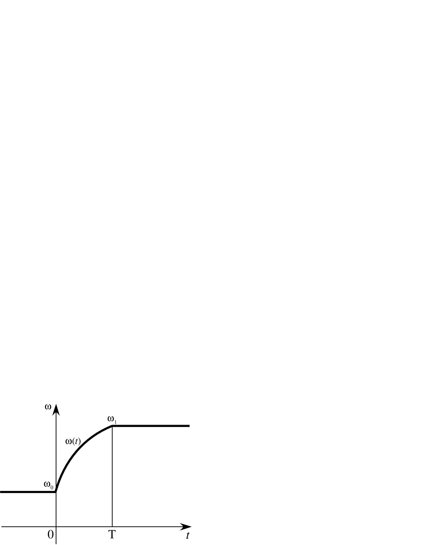
Figure 1. The parametric oscillator frequency.

9. Quantum Parametric Oscillator: General Case

The general case of the parametric oscillator with a variable frequency of the form:

$$\omega\left(t\right)=\left\{\begin{array}[]{ll}\omega_{0},&t\leq 0\vskip 6.0pt plus 2.0pt minus 2.0pt,\\ \omega\left(t\right),&0\leq t\leq T\vskip 6.0pt plus 2.0pt minus 2.0pt,\\ \omega_{1},&t\geq T\vskip 6.0pt plus 2.0pt minus 2.0pt\end{array}\right.\qquad\omega_{0}=\omega\left(0\right),\quad\omega\left(T\right)=\omega_{1}$$ (9.1)

(see Figure 1) can be investigated in a similar fashion. By the method of Ref. [20] the corresponding transition Green function is given by

$$G\left(x,y,t\right)=\frac{1}{\sqrt{2\pi i\mu\left(t\right)}}\exp\left(i\frac{m}{2\hslash}\left(\alpha\left(t\right)x^{2}+\beta\left(t\right)xy+\gamma\left(t\right)y^{2}\right)\right),\qquad 0\leq t\leq T,$$ (9.2)

where $\mu=\mu\left(t\right)$ is a solution of the equation of motion for the classical parametric oscillator [40], [45]:

$$\mu^{\prime\prime}+\omega^{2}\left(t\right)\mu=0,$$ (9.3)

that satisfies the initial conditions $\mu\left(0\right)=0$ and $\mu^{\prime}\left(0\right)=$ $\hslash/m.$ The coefficients of the quadratic form are

$$\alpha\left(t\right)=\frac{\mu^{\prime}\left(t\right)}{\mu\left(t\right)},\qquad\beta\left(t\right)=-\frac{2\hslash}{m\mu\left(t\right)},$$ (9.4)

$$\gamma\left(t\right)=\frac{\hslash^{2}}{m^{2}}\left(\frac{1}{\mu\left(t\right)\mu^{\prime}\left(t\right)}-\int_{0}^{t}\frac{\omega^{2}\left(\tau\right)}{\left(\mu^{\prime}\left(\tau\right)\right)^{2}}\ d\tau\right).$$ (9.5)

The asymptotics (8.13) hold as $t\rightarrow 0^{+};$ see Ref. [63] for more details.

A similar calculation gives the wave function (8.18) during the transition period $0<t\leq T$ as follows

$$\Psi_{n}\left(x,t\right) = \left(\dfrac{\hslash\omega_{0}}{\pi m}\right)^{1/4}\frac{1}{\sqrt{\mu\ 2^{n}n!\left(\gamma+i\omega_{0}\right)}}\left(\frac{\gamma-i\omega_{0}}{\gamma+i\omega_{0}}\right)^{n/2}$$

$$\times\exp\left(i\frac{m}{2\hslash}\left(\alpha-\frac{\beta^{2}\gamma}{4\left(\gamma^{2}+\omega_{0}^{2}\right)}\right)x^{2}\right)$$

$$\times\exp\left(-\frac{m\omega_{0}\beta^{2}x^{2}}{8\hslash\left(\gamma^{2}+\omega_{0}^{2}\right)}\right)\ H_{n}\left(\sqrt{\dfrac{m\omega_{0}}{4\hslash\left(\gamma^{2}+\omega_{0}^{2}\right)}}\ \beta x\right).$$

It satisfies the normalization condition (8.23). The continuity property $\Psi_{n}\left(x,t\right)\rightarrow\Psi_{n}^{\left(0\right)}\left(x,0\right)$ holds as $t\rightarrow 0^{+}$ for the principal branch of the radicals.

The transition amplitudes (8.24) are $c_{kn}\left(T\right)=0,$ if $k+n$ is odd, and

$$c_{kn}\left(T\right) = \Gamma\left(\frac{k+n+1}{2}\right)\left(\frac{\omega_{0}\omega_{1}}{\pi^{2}}\right)^{1/4}\sqrt{\frac{2^{k+n+1}\hslash}{\mu\ k!n!\left(\gamma+i\omega_{0}\right)m}}\left(\frac{\gamma-i\omega_{0}}{\gamma+i\omega_{0}}\right)^{n/2}$$ (9.10)

$$\times\left(\omega_{1}-\frac{\omega_{0}\beta^{2}}{4\left(\gamma^{2}+\omega_{0}^{2}\right)}+i\left(\alpha-\frac{\beta^{2}\gamma}{4\left(\gamma^{2}+\omega_{0}^{2}\right)}\right)\right)^{k/2}$$

$$\times\left(-\omega_{1}+\frac{\omega_{0}\beta^{2}}{4\left(\gamma^{2}+\omega_{0}^{2}\right)}+i\left(\alpha-\frac{\beta^{2}\gamma}{4\left(\gamma^{2}+\omega_{0}^{2}\right)}\right)\right)^{n/2}$$

$$\times\left(\omega_{1}+\frac{\omega_{0}\beta^{2}}{4\left(\gamma^{2}+\omega_{0}^{2}\right)}-i\left(\alpha-\frac{\beta^{2}\gamma}{4\left(\gamma^{2}+\omega_{0}^{2}\right)}\right)\right)^{-\left(k+n+1\right)/2}$$

$$\times~{}_{2}F_{1}\left(\begin{array}[]{c}-k,\quad-n\\ \dfrac{1}{2}\left(1-k-n\right)\end{array};\quad\frac{1}{2}\left(1+i\zeta\right)\right),$$

where

$$\zeta=\frac{\beta\sqrt{\omega_{0}\omega_{1}}}{\sqrt{\left(\alpha\omega_{0}-\gamma\omega_{1}\right)^{2}+\left(\omega_{0}\omega_{1}+\alpha\gamma-\beta^{2}/4\right)^{2}}},$$ (9.11)

if $k+n$ is even. The transformation (8.36) is applied and the unitarity of the time evolution operator implies once again the discrete orthogonality relation (8.44) for the ${}_{2}F_{1}$ functions. Their relations with Meixner polynomials and Bargmann’s functions are discussed in section 10.

For the oscillator initially in the ground state $\left(\omega_{0},0\right)$ the transition probability of finding the oscillator in the $n$th excited energy eigenstate $\left(\omega_{1},n\right)$ with the new frequency is given by $\left|c_{2k+1,0}\left(T\right)\right|^{2}=0$ and

$$\left|c_{2k,0}\left(T\right)\right|^{2} = \frac{\left|\beta\right|\sqrt{\omega_{0}\omega_{1}}}{\sqrt{\left(\alpha\omega_{0}+\gamma\omega_{1}\right)^{2}+\left(\omega_{0}\omega_{1}-\alpha\gamma+\beta^{2}/4\right)^{2}}}$$

$$\times\frac{\left(1/2\right)_{k}}{k!}\left(\frac{\left(\alpha\omega_{0}-\gamma\omega_{1}\right)^{2}+\left(\omega_{0}\omega_{1}+\alpha\gamma-\beta^{2}/4\right)^{2}}{\left(\alpha\omega_{0}+\gamma\omega_{1}\right)^{2}+\left(\omega_{0}\omega_{1}-\alpha\gamma+\beta^{2}/4\right)^{2}}\right)^{k},$$

where $k=0,1,2,...\$and $\sum_{k=0}^{\infty}\left|c_{2k,0}\left(T\right)\right|^{2}=1.$ For the oscillator initially in the first excited state $\left(\omega_{0},1\right)$ the transition probability of finding the oscillator in the $n$th excited state $\left(\omega_{1},n\right)$ is given by $\left|c_{2k,1}\left(T\right)\right|^{2}=0$ and

$$\left|c_{2k+1,1}\left(T\right)\right|^{2} = \left(\frac{\beta^{2}\omega_{0}\omega_{1}}{\left(\alpha\omega_{0}+\gamma\omega_{1}\right)^{2}+\left(\omega_{0}\omega_{1}-\alpha\gamma+\beta^{2}/4\right)^{2}}\right)^{3/2}$$

$$\times\frac{\left(3/2\right)_{k}}{k!}\left(\frac{\left(\alpha\omega_{0}-\gamma\omega_{1}\right)^{2}+\left(\omega_{0}\omega_{1}+\alpha\gamma-\beta^{2}/4\right)^{2}}{\left(\alpha\omega_{0}+\gamma\omega_{1}\right)^{2}+\left(\omega_{0}\omega_{1}-\alpha\gamma+\beta^{2}/4\right)^{2}}\right)^{k},$$

where $k=0,1,2,...\$and $\sum_{k=0}^{\infty}\left|c_{2k,0}\left(T\right)\right|^{2}=1.$ Once again, these probabilities are two special cases of the negative binomial distribution, which gives the normalized weight function for the Meixner polynomials of a discrete variable [3], [4], [24], [52], [53], and [68].

In a similar fashion, the probability that the oscillator initially in eigenstate $\left(\omega_{0},n\right)$ is found at time $T$ after the transition in state $\left(\omega_{1},k\right)$ is given by $\left|c_{kn}\left(T\right)\right|^{2}=0,$ if $k+n$ is odd, and

$$\left|c_{kn}\left(T\right)\right|^{2} = \frac{\left|\beta\right|\sqrt{\omega_{0}\omega_{1}}}{\sqrt{\left(\alpha\omega_{0}+\gamma\omega_{1}\right)^{2}+\left(\omega_{0}\omega_{1}-\alpha\gamma+\beta^{2}/4\right)^{2}}}$$ (9.17)

$$\times\frac{2^{k+n}}{k!n!\pi}\Gamma^{2}\left(\frac{k+n+1}{2}\right)$$

$$\times\left(\frac{\left(\alpha\omega_{0}-\gamma\omega_{1}\right)^{2}+\left(\omega_{0}\omega_{1}+\alpha\gamma-\beta^{2}/4\right)^{2}}{\left(\alpha\omega_{0}+\gamma\omega_{1}\right)^{2}+\left(\omega_{0}\omega_{1}-\alpha\gamma+\beta^{2}/4\right)^{2}}\right)^{\left(k+n\right)/2}$$

$$\times\left|~{}_{2}F_{1}\left(\begin{array}[]{c}-k,\quad-n\\ \dfrac{1}{2}\left(1-k-n\right)\end{array};\quad\frac{1}{2}\left(1+i\zeta\right)\right)\right|^{2},$$

if $k+n$ is even. The transformation (8.36) is valid once again but the square of the hypergeometric function can be simplified to a single positive sum with the help of a quadratic transformation (13.1) followed by the Clausen formula (13.14):

$$\left|~{}_{2}F_{1}\left(\begin{array}[]{c}-k,\quad-n\\ \dfrac{1}{2}\left(1-k-n\right)\end{array};\quad\frac{1}{2}\left(1+i\zeta\right)\right)\right|^{2}$$ (9.20)

$$\qquad=\left({}_{2}F_{1}\left(\begin{array}[]{c}-k/2,\quad-n/2\vskip 6.0pt plus 2.0pt minus 2.0pt\\ \left(1-k-n\right)/2\end{array};\quad 1+\zeta^{2}\right)\right)^{2}$$ (9.23)

$$\qquad=~{}_{3}F_{2}\left(\begin{array}[]{c}-k,\quad-n,\quad-\left(k+n\right)/2\vskip 6.0pt plus 2.0pt minus 2.0pt\\ \left(1-k-n\right)/2,\quad-k-n\end{array};\quad z\right),$$ (9.26)

where

$$z=1+\zeta^{2}=\frac{\left(\alpha\omega_{0}+\gamma\omega_{1}\right)^{2}+\left(\omega_{0}\omega_{1}-\alpha\gamma+\beta^{2}/4\right)^{2}}{\left(\alpha\omega_{0}-\gamma\omega_{1}\right)^{2}+\left(\omega_{0}\omega_{1}+\alpha\gamma-\beta^{2}/4\right)^{2}}.$$ (9.27)

Thus substituting (9.20)–(9.27) into (9.17) one gets the final representation of the probability $\left|c_{kn}\left(T\right)\right|^{2}$ in terms of a positive terminating $~{}_{3}F_{2}$ generalized hypergeometric function.

For an arbitrary initial data in $L^{2}\left(\boldsymbol{R}\right):$

$$\Psi^{\left(0\right)}\left(x,0\right)=\sum_{n=0}^{\infty}c_{n}^{\left(0\right)}\ \Psi_{n}^{\left(0\right)}\left(x,0\right),\qquad\sum_{n=0}^{\infty}\left|c_{n}^{\left(0\right)}\right|^{2}=1,$$ (9.28)

the wave function after the transition is given by

$$\Psi^{\left(1\right)}\left(x,T\right) = \int_{-\infty}^{\infty}G\left(x,y,T\right)\ \Psi^{\left(0\right)}\left(y,0\right)\ dy$$

$$= \sum_{n=0}^{\infty}c_{n}^{\left(0\right)}\int_{-\infty}^{\infty}G\left(x,y,T\right)\ \Psi_{n}^{\left(0\right)}\left(y,0\right)\ dy$$

$$= \sum_{n=0}^{\infty}c_{n}^{\left(0\right)}\Psi_{n}\left(y,T\right)=\sum_{n=0}^{\infty}c_{k}^{\left(1\right)}\Psi_{k}^{\left(1\right)}\left(x,T\right)$$

with

$$c_{k}^{\left(1\right)}=\sum_{n=0}^{\infty}c_{kn}\left(T\right)\ c_{n}^{\left(0\right)}$$ (9.30)

by (8.19). A group theoretical interpretation will be given in the next section. The orthogonality property of the transition amplitudes (8.44) implies the conservation law of the total probability

$$\sum_{k=0}^{\infty}\left|c_{k}^{\left(1\right)}\right|^{2}=\sum_{n=0}^{\infty}\left|c_{n}^{\left(0\right)}\right|^{2}=1,$$ (9.31)

which follows, of course, from the conservation of the norm of the wave function during the transition.

Thus we have solved the problem of parametric oscillator in nonrelativistic quantum mechanics provided that the solution of the corresponding classical problem (9.3) is known. A more convenient form of the transition amplitudes (9.10) will be given in the next section in terms of Bargmann’s functions. Moreover, the quantum forced parametric oscillator can be investigated by the methods of Refs. [20], [43] and [48]. We leave the details to the reader.

10. Group Theoretical Meaning of Transition Amplitudes

The group theoretical properties of the harmonic oscillator wave functions are investigated in detail. In addition to the well-known relation with the Heisenberg–Weyl algebra of the creation and annihilation operators, the $n$-dimensional oscillator wave functions form a basis of the irreducible unitary representation of the Lie algebra of the noncompact group $SU\left(1,1\right)$ corresponding to the discrete positive series $\mathcal{D}_{+}^{j};$ see [31], [48], [52] and [60]. In this paper we are dealing with the one-dimensional case only.

Define the creation and annihilation operators:

$$a^{\dagger}\left(\omega\right)=\sqrt{\frac{m}{2\hslash\omega}}\left(\omega x-\frac{\hslash}{m}\frac{\partial}{\partial x}\right),\qquad a\left(\omega\right)=\sqrt{\frac{m}{2\hslash\omega}}\left(\omega x+\frac{\hslash}{m}\frac{\partial}{\partial x}\right),$$ (10.1)

respectively, with the commutator:

$$a\left(\omega\right)a^{\dagger}\left(\omega\right)-a^{\dagger}\left(\omega\right)a\left(\omega\right)=1$$ (10.2)

and the Hamiltonian:

$$H\left(\omega\right)=\frac{\hslash\omega}{2}\left(a\left(\omega\right)a^{\dagger}\left(\omega\right)+a^{\dagger}\left(\omega\right)a\left(\omega\right)\right).$$ (10.3)

Their actions on “stationary” oscillator wave functions,

$$\Psi_{n}\left(x\right)=\left(\frac{m\omega}{\pi\hslash}\right)^{1/4}\frac{1}{\sqrt{2^{n}n!}}\exp\left(-\frac{m\omega}{2\hslash}x^{2}\right)\ H_{n}\left(\sqrt{\frac{m\omega}{\hslash}}\ x\right),$$ (10.4)

are given by

$$a\Psi_{n}=\sqrt{n}\ \Psi_{n-1},\qquad a^{\dagger}\Psi_{n}=\sqrt{n+1}\ \Psi_{n+1}.$$ (10.5)

Introducing operators

$$J_{+}\left(\omega\right) =\frac{1}{2}\left(a^{\dagger}\left(\omega\right)\right)^{2},\qquad J_{-}\left(\omega\right)=\frac{1}{2}\left(a\left(\omega\right)\right)^{2},$$ (10.6)

$$J_{0}\left(\omega\right) =\frac{1}{4}\left(a\left(\omega\right)a^{\dagger}\left(\omega\right)+a^{\dagger}\left(\omega\right)a\left(\omega\right)\right)=\frac{1}{2\hslash\omega}H\left(\omega\right),$$ (10.7)

one can easily verify the following commutation relations:

$$\left[J_{0},J_{\pm}\right]=\pm J_{\pm},\qquad\left[J_{+},J_{-}\right]=-2J_{0}.$$ (10.8)

For the Hermitian operators

$$J_{x}=\frac{1}{2}\left(J_{+}+J_{-}\right),\qquad J_{y}=\frac{1}{2i}\left(J_{+}-J_{-}\right),\qquad J_{z}=J_{0},$$ (10.9)

we get

$$\left[J_{x},J_{y}\right]=-iJ_{z},\qquad\left[J_{y},J_{z}\right]=iJ_{x},\qquad\left[J_{z},J_{x}\right]=iJ_{y}.$$ (10.10)

These commutation rules are valid for the infinitesimal operators of the non-compact group $SU\left(1,1\right);$ see, for example, [11], [31], [48], [52], [60], and [71] for more details.

One can use a different notation for the oscillator wave functions (10.4) as follows:

$$\psi_{j\lambda}=\left\{\begin{array}[]{ll}\Psi_{2n}\left(x\right),\vskip 6.0pt plus 2.0pt minus 2.0pt&\text{if }j=-3/4\text{ and }\lambda=n+1/4,\\ \Psi_{2n+1}\left(x\right),&\text{if }j=-1/4\text{ and }\lambda=n+3/4,\end{array}\right.$$ (10.11)

where $n=0,1,2,\ ...\$and the inequality $\lambda\geq j+1$ holds. The operators $J_{\pm}$ and $J_{0}$ have an explicit form

$$J_{\pm}=\frac{1}{2}\left(\frac{m\omega}{\hslash}x^{2}-\frac{H}{\hslash\omega}\mp\frac{1}{2}\mp x\frac{\partial}{\partial x}\right),\qquad J_{0}=\frac{H}{2\hslash\omega}$$ (10.12)

and their actions on the oscillator wave functions are given by

$$J_{\pm}\psi_{j\lambda}=\sqrt{\left(\lambda\mp j\right)\left(\lambda\pm j\pm 1\right)}\ \psi_{j,\lambda\pm 1},\qquad J_{0}\psi_{j\lambda}=\lambda\psi_{j\lambda},$$ (10.13)

whence

$$J^{2}\psi_{j\lambda}=j\left(j+1\right)\psi_{j\lambda}$$ (10.14)

with $J^{2}=J_{0}^{2}+J_{0}-J_{-}J_{+}=J_{0}^{2}-J_{0}-J_{+}J_{-}\ .$ These relations coincide with the formulas that define the action of the infinitesimal operators $J_{\pm}$ and $J_{0}$ of the Lie group $SU\left(1,1\right)$ on a basis $\left|j,\lambda\right\rangle$ of the irreducible representation $\mathcal{D}_{+}^{j}$ belonging to the discrete positive series in an abstract Hilbert space [11]. Thus the even and odd wave functions $\Psi_{n}\left(x\right)$ of the one-dimensional harmonic oscillator form, respectively, bases for the two irreducible representations $\mathcal{D}_{+}^{j}$ of the algebra $SU\left(1,1\right)$ with the moments $j=-3/4$ for the even values of $n$ and $j=-1/4$ for odd $n.$ It corresponds to the double valued representations of the group $SU\left(1,1\right),$ or quadruple valued representations of the $SO\left(2,1\right);$ see [52] and [60] for more details. It is important for the purpose of this paper that these group theoretical properties are valid “instantaneously”, when $\omega=\omega\left(t\right)$ is an arbitrary function of time.

As a result of an elementary, but rather tedious, calculation our transition amplitudes (9.10) can be rewritten in the form

$$c_{kn}\left(T\right)=T_{\lambda\lambda^{\prime}}^{j}\left(\theta,\tau,\varphi\right)$$ (10.15)

with the new $SU\left(1,1\right)$ quantum numbers

$$j=-\frac{3}{4},\qquad\lambda=r+\frac{1}{4},\qquad\lambda^{\prime}=s+\frac{1}{4},$$ (10.16)

if $k=2r,$ $n=2s,$ and

$$j=-\frac{1}{4},\qquad\lambda=r+\frac{3}{4},\qquad\lambda^{\prime}=s+\frac{3}{4},$$ (10.17)

if $k=2r+1,$ $n=2s+1.$ The matrix elements $T_{\lambda\lambda^{\prime}}^{j}\left(\theta,\tau,\varphi\right)$ are the so-called Bargmann functions, or the generalized spherical harmonics of $SU\left(1,1\right)$ [11], [52] and [71]:

$$T_{\lambda\lambda^{\prime}}^{j}\left(\theta,\tau,\varphi\right)=e^{-i\lambda\theta}t_{\lambda\lambda^{\prime}}^{j}\left(\tau\right)e^{-i\lambda^{\prime}\varphi}.$$ (10.18)

Here

$$t_{\lambda\lambda^{\prime}}^{j}\left(\tau\right)=\frac{\left(-1\right)^{\lambda-j-1}}{\Gamma\left(2j+2\right)}\sqrt{\frac{\Gamma\left(\lambda+j+1\right)\Gamma\left(\lambda^{\prime}+j+1\right)}{\left(\lambda-j-1\right)!\left(\lambda^{\prime}-j-1\right)!}}\ \left(\sinh\frac{\tau}{2}\right)^{-2j-2}\left(\tanh\frac{\tau}{2}\right)^{\lambda+\lambda^{\prime}}$$ (10.19)

$$\ \ \ \ \qquad\qquad\times\ \ _{2}F_{1}\left(\begin{array}[]{c}-\lambda+j+1,\ -\lambda^{\prime}+j+1\vskip 6.0pt plus 2.0pt minus 2.0pt\\ 2j+2\end{array};\ -\frac{1}{\sinh^{2}\left(\tau/2\right)}\right)$$ (10.22)

and the corresponding angles are given by

$$\tan\theta = \frac{2\alpha\omega_{0}^{2}\omega_{1}+2\gamma\omega_{1}\left(\alpha\gamma-\beta^{2}/4\right)}{\left(\alpha\omega_{0}+\gamma\omega_{1}\right)\left(\alpha\omega_{0}-\gamma\omega_{1}\right)-\left(\omega_{0}\omega_{1}+\alpha\gamma-\beta^{2}/4\right)\left(\omega_{0}\omega_{1}-\alpha\gamma+\beta^{2}/4\right)},$$ (10.23)

$$\tan\varphi = \frac{-2\gamma\omega_{0}\omega_{1}^{2}-2\alpha\omega_{0}\left(\alpha\gamma-\beta^{2}/4\right)}{\left(\alpha\omega_{0}+\gamma\omega_{1}\right)\left(\alpha\omega_{0}-\gamma\omega_{1}\right)+\left(\omega_{0}\omega_{1}+\alpha\gamma-\beta^{2}/4\right)\left(\omega_{0}\omega_{1}-\alpha\gamma+\beta^{2}/4\right)}$$ (10.24)

for two Euclidean rotations, and

$$\tanh^{2}\left(\frac{\tau}{2}\right)=\frac{\left(\alpha\omega_{0}-\gamma\omega_{1}\right)^{2}+\left(\omega_{0}\omega_{1}+\alpha\gamma-\beta^{2}/4\right)^{2}}{\left(\alpha\omega_{0}+\gamma\omega_{1}\right)^{2}+\left(\omega_{0}\omega_{1}-\alpha\gamma+\beta^{2}/4\right)^{2}}$$ (10.25)

for the hyperbolic one. The branch of the radical is taken such that

$$\frac{1}{\sinh\left(\tau/2\right)}=\frac{\beta\omega_{0}\omega_{1}}{\sqrt{\left(\alpha\omega_{0}-\gamma\omega_{1}\right)^{2}+\left(\omega_{0}\omega_{1}+\alpha\gamma-\beta^{2}/4\right)^{2}}}.$$ (10.26)

The following symmetry holds: if $\alpha\leftrightarrow\gamma$ and $\omega_{0}\leftrightarrow\omega_{1},$ then $\theta\leftrightarrow\varphi.$ It interchanges the initial and terminal oscillator states.

Our formulas (10.15)–(10.26) give a clear group theoretical interpretation of the transition amplitudes for the parametric oscillator in quantum mechanics:

$$c_{kn}\left(T\right) = \left\langle\Psi_{k}^{\left(1\right)}\left|U\left(T\right)\Psi_{n}^{\left(0\right)}\right.\right\rangle$$

$$= \left\langle\psi_{j\lambda}^{\left(1\right)}\left|T\left(\theta,\tau,\varphi\right)\psi_{j\lambda^{\prime}}^{\left(0\right)}\right.\right\rangle$$

$$= \left\langle\psi_{j\lambda}^{\left(1\right)}\left|e^{-i\theta J_{0}\left(\omega_{1}\right)}e^{-i\left(\tau+\ln\left(\omega_{1}/\omega_{0}\right)\right)J_{y}}e^{-i\varphi J_{0}\left(\omega_{0}\right)}\psi_{j\lambda^{\prime}}^{\left(0\right)}\right.\right\rangle$$

$$= e^{-i\lambda\theta}\left\langle\psi_{j\lambda}^{\left(1\right)}\left|e^{-i\left(\tau+\ln\left(\omega_{1}/\omega_{0}\right)\right)J_{y}}\psi_{j\lambda^{\prime}}^{\left(0\right)}\right.\right\rangle e^{-i\lambda^{\prime}\varphi}$$

$$= T_{\lambda\lambda^{\prime}}^{j}\left(\theta,\tau,\varphi\right),$$

if $k+n$ is even, in terms of the generalized spherical harmonics of the $SU\left(1,1\right)$ algebra for the discrete positive series $\mathcal{D}_{+}^{j}$ with $j=-3/4$ and $j=-1/4$ for the even and odd oscillator functions respectively. Formula (9.30) gives a transformation of the “coordinates” of a wave function from the old basis to the new one.

The time evolution operator has a familiar form

$$U\left(t\right)=T\left(\theta,\tau,\varphi\right)=e^{-i\theta J_{0}\left(\omega\right)}e^{-i\left(\tau+\ln\left(\omega/\omega_{0}\right)\right)J_{y}}e^{-i\varphi J_{0}\left(\omega_{0}\right)}$$ (10.28)

in terms of the corresponding infinitesimal operators, where

$$-iJ_{y}=\frac{1}{4}+\frac{1}{2}x\frac{\partial}{\partial x}.$$ (10.29)

The action of the hyperbolic rotation operator, or Lorentz boost, on a wave function is given by

$$e^{-i\tau J_{y}}\psi\left(x\right)=e^{\tau/4}\psi\left(e^{\tau/2}x\right).$$ (10.30)

Therefore,

$$t_{\lambda\lambda^{\prime}}^{j}\left(\tau\right) = \left\langle\psi_{j\lambda}^{\left(1\right)}\left|e^{-i\tau J_{y}}\psi_{j\lambda^{\prime}}^{\left(1\right)}\right.\right\rangle$$

$$= e^{\tau/4}\int_{-\infty}^{\infty}\Psi_{k}^{\left(1\right)}\left(x\right)\ \Psi_{n}^{\left(1\right)}\left(e^{\tau/2}x\right)\ dx,$$

if $k+n$ is even, which gives an integral representation for the Bargmann function under consideration; cf. [52].

Thus the $SU\left(1,1\right)$ symmetry suggests the following algebraic form

$$U\left(t\right) = \exp\left(\frac{i\theta}{2\hslash\omega}\left(\frac{\hslash^{2}}{2m}\frac{\partial^{2}}{\partial x^{2}}-\frac{m\omega^{2}}{2}x^{2}\right)\right)$$

$$\times\exp\left(\frac{\tau+\ln\left(\omega/\omega_{0}\right)}{2}\left(\frac{1}{2}+x\frac{\partial}{\partial x}\right)\right)$$

$$\times\exp\left(\frac{i\varphi}{2\hslash\omega_{0}}\left(\frac{\hslash^{2}}{2m}\frac{\partial^{2}}{\partial x^{2}}-\frac{m\omega_{0}^{2}}{2}x^{2}\right)\right)$$

of the time evolution operator, where the group parameters $\theta,$ $\tau,$ $\varphi$ are governed by the oscillator transition dynamics through formulas (10.23)–(10.26) back to the classical equation of motion for the parametric oscillator (9.3).

It is worth noting that Bargmann’s functions are studied in detail. The functions $t_{\lambda\lambda^{\prime}}^{j}\left(\tau\right)$ are related to the Meixner polynomials — the unitarity property of the Bargmann functions,

$$\sum_{\lambda^{\prime\prime}=j+1}^{\infty}t_{\lambda\lambda^{\prime\prime}}^{j}\left(\tau\right)t_{\lambda^{\prime}\lambda^{\prime\prime}}^{j}\left(\tau\right)=\delta_{\lambda\lambda^{\prime}},$$ (10.33)

gives the discrete orthogonality relation of these polynomials. A connection with a finite set of Jacobi polynomials orthogonal on an infinite interval is also relevant. All basic facts about the functions $T_{\lambda\lambda^{\prime}}^{j}\left(\theta,\tau,\varphi\right)$ can be derived from the well-known properties of the Meixner and Jacobi polynomials; see Refs. [52], [61], and [71] for more details.

11. Summary

The time-dependent Schrödinger equations with variable coefficients

$$i\frac{\partial\psi}{\partial t}+\frac{1}{4}\frac{\partial^{2}\psi}{\partial x^{2}}\pm tx^{2}\psi=0$$ (11.1)

have the Green functions of the form

$$G\left(x,y,t\right)=\frac{1}{\sqrt{\pm\pi ia\left(\pm t\right)}}\exp\left(\pm i\frac{a^{\prime}\left(\pm t\right)-2xy+b\left(\pm t\right)y^{2}}{a\left(\pm t\right)}\right),\qquad t>0,$$ (11.2)

where $a\left(t\right)=ai\left(t\right)$ and $b\left(t\right)=bi\left(t\right)$ are solutions of the Airy equation $\mu^{\prime\prime}-t\mu=0$ that satisfy the initial conditions $a\left(0\right)=b^{\prime}\left(0\right)=0$ and $a^{\prime}\left(0\right)=b\left(0\right)=1;$ see Appendix A below for construction of these solutions.

In the momentum representation the corresponding Schrödinger equations with variable coefficients

$$i\frac{\partial\psi}{\partial t}\mp t\frac{\partial^{2}\psi}{\partial x^{2}}-\frac{1}{4}x^{2}\psi=0$$ (11.3)

have the Green functions of the form

$$G\left(x,y,t\right)=\frac{1}{\sqrt{\mp 4\pi ib^{\prime}\left(\pm t\right)}}\exp\left(\mp i\frac{b\left(\pm t\right)-2xy+a^{\prime}\left(\pm t\right)y^{2}}{4b^{\prime}\left(\pm t\right)}\right),\qquad t>0,$$ (11.4)

where $a^{\prime}\left(t\right)=ai^{\prime}\left(t\right)$ and $b^{\prime}\left(t\right)=bi^{\prime}\left(t\right)$ are solutions of the equation $\mu^{\prime\prime}-\left(1/t\right)\mu^{\prime}-t\mu=0$ that satisfy the initial conditions $a^{\prime}\left(0\right)=1$ and $b^{\prime}\left(0\right)=0;$ see Appendix A for further properties of these functions.

Solution of the corresponding Cauchy initial value problem is given by the time evolution operator as follows

$$\psi\left(x,t\right)=\int_{-\infty}^{\infty}G\left(x,y,t\right)\ \varphi\left(y\right)\ dy,\qquad\psi\left(x,0\right)=\varphi\left(x\right)$$ (11.5)

for a suitable function $\varphi$ on $\boldsymbol{R};$ see Ref. [63] for more details. Additional integrable cases are given with the help of the gauge transformation.

Particular solutions of the corresponding nonlinear Schrödinger equations are obtained by the methods of Refs. [20] and [22]. A special case of the quantum parametric oscillator with the Hamiltonian of the form (8.3) is studied in detail. The Green function is explicitly evaluated in terms of Airy functions by equations (8.7)–(8.11) and the corresponding transition amplitudes are given in terms of a hypergeometric function by formula (8.32). A discrete orthogonality relation for certain ${}_{2}F_{1}$ functions is derived from the fundamentals of quantum physics. It is identified then as orthogonality property of special Meixner polynomials with the help of a quadratic transformation. An extension to the general case of parametric oscillator in quantum mechanics is also given. Relation of the transition amplitudes with unitary irreducible representations of the Lorentz group $SU\left(1,1\right)$ is established. Further extension to the quantum forced parametric oscillator is left to the reader.

We dedicate this paper to Professor Richard Askey on his 75th birthday for his outstanding contributions to the area of classical analysis, special functions and their numerous applications, and mathematical education.

12. Appendix A: Solutions of Airy Equation

Bessel functions are defined as

$$J_{\nu}\left(z\right)=\left(\frac{z}{2}\right)^{\nu}\sum_{k=0}^{\infty}\frac{\left(-z^{2}/4\right)^{k}}{k!\Gamma\left(\nu+k+1\right)}$$ (12.1)

and the modified Bessel functions are

$$I_{\nu}\left(z\right)=\left(\frac{z}{2}\right)^{\nu}\sum_{k=0}^{\infty}\frac{\left(z^{2}/4\right)^{k}}{k!\Gamma\left(\nu+k+1\right)}.$$ (12.2)

For an extensive theory of these functions, see Refs. [1], [3], [53], [56], [67], [72] and references therein.

The Airy functions satisfy the second order differential equation

$$u^{\prime\prime}-tu=0.$$ (12.3)

Their standard definitions are

$$Ai\left(t\right) = \frac{\sqrt{t}}{3}\left(I_{-1/3}\left(z\right)-I_{1/3}\left(z\right)\right),$$ (12.4)

$$Bi\left(t\right) = \sqrt{\frac{t}{3}}\left(I_{-1/3}\left(z\right)+I_{1/3}\left(z\right)\right)$$ (12.5)

and

$$Ai\left(-t\right) = \frac{\sqrt{t}}{3}\left(J_{-1/3}\left(z\right)+J_{1/3}\left(z\right)\right),$$ (12.6)

$$Bi\left(-t\right) = \sqrt{\frac{t}{3}}\left(J_{-1/3}\left(z\right)-J_{1/3}\left(z\right)\right)$$ (12.7)

with $z=\left(2/3\right)t^{3/2}.$ The Wronskian is equal to

$$W\left(Ai\left(t\right),Bi\left(t\right)\right)=\frac{1}{\pi}$$ (12.8)

and the derivatives are given by

$$Ai^{\prime}\left(t\right) = \frac{\sqrt{t}}{3}\left(I_{2/3}\left(z\right)-I_{-2/3}\left(z\right)\right),$$ (12.9)

$$Bi^{\prime}\left(t\right) = \sqrt{\frac{t}{3}}\left(I_{2/3}\left(z\right)+I_{-2/3}\left(z\right)\right)$$ (12.10)

and

$$Ai^{\prime}\left(-t\right) = \frac{t}{3}\left(J_{2/3}\left(z\right)-J_{-2/3}\left(z\right)\right),$$ (12.11)

$$Bi^{\prime}\left(-t\right) = \frac{t}{\sqrt{3}}\left(J_{2/3}\left(z\right)+J_{-2/3}\left(z\right)\right)$$ (12.12)

with $z=\left(2/3\right)t^{3/2}.$

In this paper we use the following pair of linearly independent solutions

$$a\left(t\right) = ai\left(t\right)=\frac{1}{3^{2/3}}\Gamma\left(\frac{1}{3}\right)t^{1/2}I_{1/3}\left(\frac{2}{3}t^{3/2}\right)$$

$$= t\sum_{k=0}^{\infty}\frac{\left(t^{3}/9\right)^{k}}{k!\left(4/3\right)_{k}}=\sum_{k=0}^{\infty}3^{k}\left(\frac{2}{3}\right)_{k}\frac{t^{3k+1}}{\left(3k+1\right)!}$$

$$= t+\frac{t^{4}}{2^{2}3}+\frac{t^{7}}{2^{3}3^{2}7}+...$$

and

$$b\left(t\right) = bi\left(t\right)=\frac{1}{3^{1/3}}\Gamma\left(\frac{2}{3}\right)t^{1/2}I_{-1/3}\left(\frac{2}{3}t^{3/2}\right)$$

$$= \sum_{k=0}^{\infty}\frac{\left(t^{3}/9\right)^{k}}{k!\left(2/3\right)_{k}}=\sum_{k=0}^{\infty}3^{k}\left(\frac{1}{3}\right)_{k}\frac{t^{3k}}{\left(3k\right)!}$$

$$= 1+\frac{t^{3}}{6}+\frac{t^{6}}{2^{2}3^{2}5}+...$$

with $a\left(0\right)=b^{\prime}\left(0\right)=0,$ $a^{\prime}\left(0\right)=b\left(0\right)=1.$ Their relations with the standard Airy functions $Ai\left(t\right)$ and $Bi\left(t\right)$ are

$$\left(\begin{array}[]{c}a\left(t\right)\\ b\left(t\right)\end{array}\right)=\frac{1}{2}\left(\begin{array}[]{cc}-3^{1/3}\Gamma\left(1/3\right)&3^{-1/6}\Gamma\left(1/3\right)\\ 3^{2/3}\Gamma\left(2/3\right)&3^{1/6}\Gamma\left(2/3\right)\end{array}\right)\left(\begin{array}[]{c}Ai\left(t\right)\\ Bi\left(t\right)\end{array}\right)$$ (12.15)

with the inverse

$$\left(\begin{array}[]{c}Ai\left(t\right)\\ Bi\left(t\right)\end{array}\right)=\frac{1}{\pi}\left(\begin{array}[]{cc}-3^{1/6}\Gamma\left(2/3\right)&3^{-1/6}\Gamma\left(1/3\right)\\ 3^{2/3}\Gamma\left(2/3\right)&3^{1/3}\Gamma\left(1/3\right)\end{array}\right)\left(\begin{array}[]{c}a\left(t\right)\\ b\left(t\right)\end{array}\right)$$ (12.16)

and the Wronskian is

$$W\left(a\left(t\right),b\left(t\right)\right)=-1.$$ (12.17)

The derivatives are given by

$$a^{\prime}\left(t\right) = ai^{\prime}\left(t\right)=\frac{1}{3^{2/3}}\Gamma\left(\frac{1}{3}\right)tI_{-2/3}\left(\frac{2}{3}t^{3/2}\right)$$

$$= \sum_{k=0}^{\infty}\frac{\left(t^{3}/9\right)^{k}}{k!\left(1/3\right)_{k}}=\sum_{k=0}^{\infty}3^{k}\left(\frac{2}{3}\right)_{k}\frac{t^{3k}}{\left(3k\right)!}$$

$$= 1+\frac{t^{3}}{3}+\frac{t^{6}}{2^{3}3^{2}}+...$$

and

$$b^{\prime}\left(t\right) = bi^{\prime}\left(t\right)=\frac{1}{3^{1/3}}\Gamma\left(\frac{2}{3}\right)tI_{2/3}\left(\frac{2}{3}t^{3/2}\right)$$

$$= \frac{t^{2}}{2}\sum_{k=0}^{\infty}\frac{\left(t^{3}/9\right)^{k}}{k!\left(5/3\right)_{k}}=\sum_{k=0}^{\infty}3^{k}\left(\frac{4}{3}\right)_{k}\frac{t^{3k+2}}{\left(3k+2\right)!}$$

$$= \frac{t^{2}}{2}+\frac{t^{5}}{2^{2}3\cdot 5}+...$$

with the Wronskian

$$W\left(a^{\prime}\left(t\right),b^{\prime}\left(t\right)\right)=t.$$ (12.20)

More facts about the Airy functions can be found in Refs. [1], [53], and [54].

13. Appendix B: Some Transformations of Hypergeometric Functions

We derive the transformation formulas (8.36) as follows. In the even case $k=2r$ and $n=2s,$ use the quadratic transformation [3], [56]:

$${}_{2}F_{1}\left(\begin{array}[]{c}a,\quad b\\ a+b+\dfrac{1}{2}\end{array};\ 4z\left(1-z\right)\right)=\ _{2}F_{1}\left(\begin{array}[]{c}2a,\quad 2b\\ a+b+\dfrac{1}{2}\end{array};\ z\right)$$ (13.1)

followed by a transformation:

$$\ {}_{2}F_{1}\left(\begin{array}[]{c}a,\ -r\\ c\end{array};\ z\right)=\frac{\left(c-a\right)_{r}}{\left(c\right)_{r}}\ \ _{2}F_{1}\left(\begin{array}[]{c}a,\quad-r\\ 1+a-c-r\end{array};\ 1-z\right),$$ (13.2)

where $\left(a\right)_{r}=a\left(a+1\right)...\left(a+r-1\right)=\Gamma\left(a+r\right)/\Gamma\left(a\right),$ for the terminating hypergeometric function. The reflection formula for gamma function:

$$\Gamma\left(z\right)\Gamma\left(1-z\right)=\frac{\pi}{\sin\pi z}$$ (13.3)

allows to complete the proof.

In the odd case $k=2r+1$ and $n=2s+1,$ one can use the quadratic transformation (13.1) for pure imaginary values of $\zeta$ with $0<\left(\mathop{\mathrm{I}m}\zeta\right)^{2}<2,$ when the series converges. Apply the familiar transformation [3], [53], [56]:

$$\ {}_{2}F_{1}\left(\begin{array}[]{c}a,\ b\\ c\end{array};\ z\right)=\left(1-z\right)^{c-a-b}\ _{2}F_{1}\left(\begin{array}[]{c}c-a,\quad c-b\\ c\end{array};\ z\right)$$ (13.4)

to get back to a terminating hypergeometric function. The end result, namely,

$${}_{2}F_{1}\left(\begin{array}[]{c}-2r-1,\ -2s-1\vskip 6.0pt plus 2.0pt minus 2.0pt\\ -r-s-1/2\end{array};\ \dfrac{1}{2}\left(1+i\zeta\right)\right)$$ (13.7)

$$\quad=\ _{2}F_{1}\left(\begin{array}[]{c}-r-1/2,\ -s-1/2\vskip 6.0pt plus 2.0pt minus 2.0pt\\ -r-s-1/2\end{array};\ 1+\zeta^{2}\right)$$ (13.10)

$$\quad\quad=-i\zeta\ _{2}F_{1}\left(\begin{array}[]{c}-r,\ -s\vskip 6.0pt plus 2.0pt minus 2.0pt\\ -r-s-1/2\end{array};\ 1+\zeta^{2}\right),$$ (13.13)

is valid by analytic continuation in the entire complex plane. Our choice of the branch of the radical corresponds to the correct special value at $r=s=0.$ Use the transformation (13.2) and reflection formula (13.3) in order to complete the proof.

The Clausen formula [3]:

$$\left[{}_{2}F_{1}\left(\begin{array}[]{c}a,\quad b\\ a+b+\dfrac{1}{2}\end{array};\ z\right)\right]^{2}=\ _{3}F_{2}\left(\begin{array}[]{c}2a,\quad 2b,\quad a+b\\ a+b+\dfrac{1}{2},\quad 2a+2b\end{array};\ z\right)$$ (13.14)

and the duplication formula for gamma function:

$$\Gamma\left(2z\right)=\frac{2^{2z-1}}{\sqrt{\pi}}\Gamma\left(z\right)\Gamma\left(z+\frac{1}{2}\right)$$ (13.15)

have been used in sections 8 and 9.

Acknowledgment. We thank Professor Richard Askey for motivation, valuable discussions and encouragement.

References

• [1] M. Abramowitz and I. A. Stegan, Handbook of Mathematical Functions, Dover Publications, New York, 1972.
• [2] G. E. Andrews and R. A. Askey, Classical orthogonal polynomials, in: “Polynômes orthogonaux et applications”, Lecture Notes in Math. 1171, Springer-Verlag, 1985, pp. 36–62.
• [3] G. E. Andrews, R. A. Askey, and R. Roy, Special Functions, Cambridge University Press, Cambridge, 1999.
• [4] R. A. Askey, Orthogonal Polynomials and Special Functions, CBMS–NSF Regional Conferences Series in Applied Mathematics, SIAM, Philadelphia, Pennsylvania, 1975.
• [5] R. A. Askey, Continuous Hahn polynomials, J. Phys. A: Math. Gen. 18 (1985), L1017–L1019.
• [6] R. A. Askey and J. A. Wilson, A set of hypergeometric orthogonal polynomials, SIAM J. Math. Anal. 13 (1982), 651–655.
• [7] R. A. Askey and J. A. Wilson, Some basic hypergeometric orthogonal polynomials that generalize Jacobi polynomials, Memoirs Amer. Math. Soc., Number 319 (1985).
• [8] G. P. Arrighini and N. L. Durante, More on the quantum propagator of a particle in a linear potential, Am. J. Phys. 64 (1996) # 8, 1036–1041.
• [9] N. M. Atakishiyev and S. K. Suslov, The Hahn and Meixner polynomials of imaginary argument and some of their applications, J. Phys. A: Math. Gen. 18 (1985), 1583–1596.
• [10] W. N. Bailey, Some integrals involving Hermite polynomials, J. London Math. Soc. 23 (1948) # 4, 291–297.
• [11] V. Bargmann, Irreducible unitary representations of the Lorentz group, Annals of Mathematics (2) 48 (1947), 568–640.
• [12] H. Bateman, Partial Differential Equations of Mathematical Physics, Dover, New York, 1944.
• [13] L. A. Beauregard, Propagators in nonrelativistic quantum mechanics, Am. J. Phys. 34 (1966), 324–332.
• [14] N. N. Bogoliubov and D. V. Shirkov, Introduction to the Theory of Quantized Fields, third edition, John Wiley & Sons, New York, Chichester, Brisbane, Toronto, 1980.
• [15] L. Brillouin, La mécanique ondulatoire de Schrödinger: une méthode générale de resolution par approximations successives, Comptes Rendes de l’Académie des Sciences, Ser. A 183 (1926), 24–26.
• [16] L. S. Brown and Y. Zhang, Path integral for the motion of a particle in a linear potential, Am. J. Phys. 62 (1994) # 9, 806–808.
• [17] J. R. Cannon, The One-Dimensional Heat Equation, Encyclopedia of Mathematics and Its Applications, Vol. 32, Addison–Wesley Publishing Company, Reading etc, 1984.
• [18] T. Cazenave, Semilinear Schrödinger Equations, Courant Lecture Notes in Mathematics, Vol. 10, American Mathematical Society, Providence, Rhode Island, 2003.
• [19] T. Cazenave and A. Haraux, An Introduction to Semilinear Evolution Equations, Oxford Lecture Series in Mathematics and Its Applications, Vol. 13, Oxford Science Publications, Claredon Press, Oxford, 1998.
• [20] R. Cordero-Soto, R. M. Lopez, E. Suazo, and S. K. Suslov, Propagator of a charged particle with a spin in uniform magnetic and perpendicular electric fields, Lett. Math. Phys. 84 (2008) #2–3, 159–178.
• [21] R. Cordero-Soto, E. Suazo, and S. K. Suslov, Models of damped oscillators in quantum mechanics, under preparation.
• [22] R. Cordero-Soto and S. K. Suslov, The time inversion for modified oscillators, arXiv:0808.3149v9 [math-ph] 8 Mar 2009.
• [23] Jean le Round d’Alembert, Equation $z^{\prime}=\varphi\left(x\right)z,z\left(a\right)=z\left(b\right)=0,y=z^{\prime}/z$, 1763 Histoire de ľAcademie de Berlin, 1770, Vol. 19, p. 224 et seq.
• [24] A. Erdélyi, Higher Transcendental Functions, Vols. I–III, A. Erdélyi, ed., McGraw–Hill, 1953.
• [25] A. Erdélyi, Tables of Integral Transforms, Vols. I–II, A. Erdélyi, ed., McGraw–Hill, 1954.
• [26] R. P. Feynman, The Principle of Least Action in Quantum Mechanics, Ph. D. thesis, Princeton University, 1942; reprinted in: “Feynman’s Thesis – A New Approach to Quantum Theory”, (L. M. Brown, Editor), World Scientific Publishers, Singapore, 2005, pp. 1–69.
• [27] R. P. Feynman, Space-time approach to non-relativistic quantum mechanics, Rev. Mod. Phys. 20 (1948) # 2, 367–387; reprinted in: “Feynman’s Thesis – A New Approach to Quantum Theory”, (L. M. Brown, Editor), World Scientific Publishers, Singapore, 2005, pp. 71–112.
• [28] R. P. Feynman, The theory of positrons, Phys. Rev. 76 (1949) # 6, 749–759.
• [29] R. P. Feynman, Space-time approach to quantum electrodynamics, Phys. Rev. 76 (1949) # 6, 769–789.
• [30] R. P. Feynman and A. R. Hibbs, Quantum Mechanics and Path Integrals, McGraw–Hill, New York, 1965.
• [31] G. F. Filippov, V. I. Ovcharenko, and Yu. F. Smirnov, Theory of Collective Excitation of Atomic Nuclei, Naukova Dumka, Kiev, 1981 [in Russian].
• [32] S. Fraga, J. M. García de la Vega, and E. S. Fraga, The Schrödinger and Riccati Equation, Lecture Notes in Chemistry, Vol. 70, Springer–Verlag, Berlin, New York, 1999.
• [33] K. Gottfried and T.-M. Yan, Quantum Mechanics: Fundamentals, second edition, Springer–Verlag, Berlin, New York, 2003.
• [34] D. R. Haaheim and F. M. Stein, Methods of solution of the Riccati differential equation, Mathematics Magazine 42 (1969) #2, 233–240.
• [35] B. R. Holstein, The linear potential propagator, Am. J. Phys. 65 (1997) #5, 414–418.
• [36] B. R. Holstein, The harmonic oscillator propagator, Am. J. Phys. 67 (1998) #7, 583–589.
• [37] R. Koekoek and R. F. Swarttouw, The Askey scheme of hypergeometric orthogonal polynomials and its $q$-analogues, Report 94–05, Delft University of Technology, 1994.
• [38] H. A. Kramers, Wellenmechanik und halbzählige Quantisierung, Zeitschrift der Physik 39 (1926), 828–840.
• [39] O. A. Ladyženskaja, V. A. Solonnikov, and N. N. Ural’ceva, Linear and Quasilinear Equations of Parabolic Type, Translations of Mathematical Monographs, Vol. 23, American Mathematical Sociaty, Providence, Rhode Island, 1968. (pp. 318, 356)
• [40] L. D. Landau and E. M. Lifshitz, Mechanics, Pergamon Press, Oxford, 1976.
• [41] L. D. Landau and E. M. Lifshitz, Quantum Mechanics: Nonrelativistic Theory, Pergamon Press, Oxford, 1977.
• [42] E. E. Levi, Sulle equazioni lineari totalmente ellittiche alle derivate parziali, Rend. Circ. Mat. Palermo 24 (1907) , 275–317.
• [43] R. M. Lopez and S. K. Suslov, The Cauchy problem for a forced harmonic oscillator, arXiv:0707.1902v8 [math-ph] 27 Dec 2007.
• [44] R. D. Lord, Some integrals involving Hermite polynomials, J. London Math. Soc. 24 (1948) # 2, 101–112.
• [45] W. Magnus and S. Winkler, Hill’s Equation, Dover Publications, New York, 1966.
• [46] V. P. Maslov and M. V. Fedoriuk, Semiclassical Approximation in Quantum Mechanics, Reidel, Dordrecht, Boston, 1981.
• [47] I. V. Melinikova and A. Filinkov, Abstract Cauchy problems: Three Approaches, Chapman&Hall/CRC, Boca Raton, London, New York, Washington, D. C., 2001.
• [48] M. Meiler, R. Cordero-Soto, and S. K. Suslov, Solution of the Cauchy problem for a time-dependent Schrödinger equation, J. Math. Phys. 49 (2008) #7, 072102: 1–27; published on line 9 July 2008, URL: http://link.aip.org/link/?JMP/49/072102; see also arXiv: 0711.0559v4 [math-ph] 5 Dec 2007.
• [49] E. Merzbacher, Quantum Mechanics, third edition, John Wiley & Sons, New York, 1998.
• [50] A. M. Molchanov, The Riccati equation $y^{\prime}=x+y^{2}$ for the Airy function, [in Russian], Dokl. Akad. Nauk 383 (2002) #2, 175–178.
• [51] P. Nardone, Heisenberg picture in quantum mechanics and linear evolutionary systems, Am. J. Phys. 61 (1993) # 3, 232–237.
• [52] A. F. Nikiforov, S. K. Suslov, and V. B. Uvarov, Classical Orthogonal Polynomials of a Discrete Variable, Springer–Verlag, Berlin, New York, 1991.
• [53] A. F. Nikiforov and V. B. Uvarov, Special Functions of Mathematical Physics, Birkhäuser, Basel, Boston, 1988.
• [54] F. W. J. Olver, Asymptotics and Special Functions, Academic Press, New York, 1974.
• [55] J. D. Paliouras and D. S. Meadows, Complex Variables for Scientists and Engineers, second edition, Macmillan Publishing Company, New York and London, 1990.
• [56] E. D. Rainville, Special Functions, The Macmillan Company, New York, 1960.
• [57] E. D. Rainville, Intermediate Differential Equations, Wiley, New York, 1964.
• [58] S. S. Rajah and S. D. Maharaj, A Riccati equation in radiative stellar collapse, J. Math. Phys. 49 (2008) #1, 012501: 1–9; published on line 23 January 2008.
• [59] R. W. Robinett, Quantum mechanical time-development operator for the uniformly accelerated particle, Am. J. Phys. 64 (1996) #6, 803–808.
• [60] Yu. F. Smirnov and K. V. Shitikova, The method of K harmonics and the shell model, Soviet Journal of Particles & Nuclei 8 (1977) #4, 344–370.
• [61] Yu. F. Smirnov, S. K. Suslov, and A. M. Shirokov, Clebsch-Gordan coefficients and Racah coefficients for the $SU\left(2\right)$ and $SU\left(1,1\right)$ groups as the discrete analogues of the Pöschl–Teller potential wavefunctions, J. Phys. A: Math. Gen. 17 (1984), 2157–2175.
• [62] E. Suazo, and S. K. Suslov, An integral form of the nonlinear Schrödinger equation with wariable coefficients, arXiv:0805.0633v2 [math-ph] 19 May 2008.
• [63] E. Suazo and S. K. Suslov, Cauchy problem for Schrödinger equation with variable quadratic Hamiltonians, under preparation.
• [64] E. Suazo, S. K. Suslov, and J. M. Vega, The Riccati differential equation and a diffusion-type equation, arXiv:0807.4349v4 [math-ph] 8 Aug 2008.
• [65] S. K. Suslov, Matrix elements of Lorentz boosts and the orthogonality of Hahn polynomials on a contour, Sov. J. Nucl. Phys. 36 (1982) #4, 621–622.
• [66] S. K. Suslov, The Hahn polynomials in the Coulomb problem, Sov. J. Nucl. Phys. 40 (1984) #1, 79–82.
• [67] S. K. Suslov and B. Trey, The Hahn polynomials in the nonrelativistic and relativistic Coulomb problems, J. Math. Phys. 49 (2008) #1, 012104: 1–51; published on line 22 January 2008, URL: http://link.aip.org/link/?JMP/49/012104.
• [68] G. Szegő, Orthogonal Polynomials, Amer. Math. Soc. Colloq. Publ., Vol. 23, Rhode Island, 1939.
• [69] T. Tao, Nonlinear Dispersive Equations: Local and Global Analysis, CBMS regional conference series in mathematics, 2006.
• [70] N. S. Thomber and E. F. Taylor, Propagator for the simple harmonic oscillator, Am. J. Phys. 66 (1998) # 11, 1022–1024.
• [71] N. Ya. Vilenkin, Special Functions and the Theory of Group Representations, American Mathematical Society, Providence, 1968.
• [72] G. N. Watson, A Treatise on the Theory of Bessel Functions, Second Edition, Cambridge University Press, Cambridge, 1944.
• [73] G. Wentzel, Eine Verallgemeinerung der Quantenbedingungen für die Zwecke der Wellenmechanik, Zeitschrift der Physik 38 (1926), 518–529.