Long-range correlations in a simple stochastic model of coupled transport

Abstract

We study coupled transport in the nonequilibrium stationary state of a model consisting of independent random walkers, moving along a one-dimensional channel, which carry a conserved energy-like quantity, with density and temperature gradients imposed by reservoirs at the ends of the channel. In our model, walkers interact with other walkers at the same site by sharing energy at each time step, but the amount of energy carried does not affect the motion of the walkers. We find that already in this simple model long-range correlations arise in the nonequilibrium stationary state which are similar to those observed in more realistic models of coupled transport. We derive an analytical expression for the source of these correlations, which we use to obtain semi-analytical results for the correlations themselves assuming a local-equilibrium hypothesis. These are in very good agreement with results from direct numerical simulations.

1 Introduction

Two related outstanding problems at the heart of nonequilibrium statistical mechanics are the structure of the probability distribution function in the stationary state, and the derivation of macroscopic transport laws, such as Fourier’s law of heat conduction, from microscopic dynamics, for systems which are maintained out of equilibrium by the imposition of thermodynamic fluxes [1, 2, 3].

For certain classes of stochastic mass-transport equations, known as zero-range processes, in which the dynamics of mass leaving a site depends only on the occupation number at that site, the stationary-state distribution is known to factorise into the product of single-site distributions under certain conditions, which enables many analytical results to be obtained [4]. However, for more complicated models, this distribution no longer factorises. In this case, the appropriate characterisation of the stationary-state distribution becomes a central goal for the description of these systems. Furthermore, the fact that the distribution does not factorise implies the existence of spatial correlations between different sites, as has been discussed in many previous works [5, 6]. These spatial correlations in nonequilibrium states have been studied at a mescoscopic level using fluctuating hydrodynamics [6]. Generically, they tend to be long-range, spanning the whole length of the system, rather than decaying exponentially as in equilibrium systems away from critical points.

From a microscopic point of view, the correlations arising in nonequilibrium stationary states have already been studied in many simple models, including a stochastic master equation describing heat flow [7], oscillators which exchange energy [8], lattice-gases with exclusion [9] [10], and lattice-gas cellular automata [11]. Also, exact results for all correlation functions were found using matrix technique for the symmetric simple exclusion process: see e.g. [12] for a recent review, where the relation of long-range correlations to a non-local free energy functional is also discussed. An approximation of the invariant measure using Gaussians in a suitably rotated coordinate system has recently been obtained [13, 14]; and related analytical results were previously found by Suárez et al. [11], for the case where transport is by particles with exclusion, but with a single conserved quantity.

In particular, long-range correlations in the so-called “random-halves” model [15] of coupled matter and heat transport were recently studied in [16], principally heuristically and numerically. The model we study in this paper can be considered to be a simplified version of the random-halves model, still containing two explicitly conserved quantities. The simplification enables us to obtain an explicit expression for the source of the correlations in the nonequilibrium stationary state of the system.

Although our model suppresses much of the physical meaning of the second conserved quantity, in addition to mass, which in [16] can really be viewed as corresponding to energy, we emphasise that the structure of the spatial correlations that we observe for this energy-like quantity is remarkably similar to that found in [16].

In this paper, we study the equilibrium and nonequilibrium stationary states of the model. In regards to the nonequilibrium stationary state, we obtain the transport equations for the energy and mass, and we obtain the equation satisfied by the spatial energy correlations that arise in the model. This equation has a non-closed form. To close the hierarchy, we make a local equilibrium assumption, which enables an analytical evaluation of the form of the correlation source terms. We are then left with an approximate discrete Poisson equation with source terms for the correlations. We find very good agreement between the solution of this equation with numerical simulations of the system.

2 Coupled transport model

In this section we introduce the model of transport which we study. It is, perhaps, one of the simplest stochastic models exhibiting coupled transport. The transported quantities are particles (mass), and a second quantity, which is locally conserved, which the particles carry with them when they move. For simplicity of exposition, we refer to this second quantity as “energy”, although we emphasise that it does not necesarily have the physical characteristics of an energy, since the motion of the walkers is independent of the value of the energy which they carry.

Specifically, the model consists of independent random walkers moving on a one-dimensional chain of $L$ sites. The system is open, and is in contact with particle and energy baths at each end of the chain, which at each time step supply or remove particles from the system with a given rate and energy distribution corresponding to their density and temperature, respectively.

The walkers move synchronously in discrete time: at each time step, each walker independently attempts to jump to one of its two neighbouring sites, or remains at the same site. If a walker successfully jumps, then it carries with it an amount of energy $s$ from the total amount of energy $E$ at its previous site.

After all particles have attempted their jumps, the total energy at each site, that is, the sum of the individual energies of the walkers at that site, is redistributed among all the particles at that site, in a “random” (microcanonical) way, which we specify below. We thus have a complete (infinite) separation of time-scales: energy equilibration at each site is completed before the particles move again. This separation of time scales is, in part, what enables us to proceed with the analysis of the system. Further, it ensures that we can always use a local equilibrium hypothesis, in the sense that all thermodynamic quantities are always well defined at every site and that they are related to each other according to the usual (equilibrium) thermodynamic relations.

As mentioned above, our model is related to the recently-introduced random-halves model [15, 16], designed to model, rather faithfully, the Hamiltonian dynamics underlying the transport phenomena observed in [17, 18]. In the random-halves model, each particle jumps to a neighbouring site with a rate which is proportional to the square root of its kinetic energy, and which is a factor $\delta$ times the rate at which a particle exchanges a random fraction of its energy with a reservoir located at its current position.

Taking the limit $\delta\to 0$ in the random-halves model corresponds to our limit of infinite separation of time-scales, the other particles at that site acting as the reservoir. However, the random-halves model includes extra effects which our model cannot account for: for example, in the random-halves model, it is possible to have sites with particles at very low energy, and since the jump rate is energy dependent, these particles may remain a long time at that site unless other very energetic particles arrive there. Nonetheless, as we shall see, these kind of effects do not appear to affect the qualitative results on correlations.

Although we do not consider it in this work, it should be noted that if we make the jump probabilities $p$ and $q$ very small (of order $1/N$, where $N$ represents the number of particles in the system) we effectively recover single-particle motion, as in continuous-time dynamics, that is, on average, only one particle moves at each time step. Furthermore, in this case we could unambiguously consider jumping probabilities that are functions of the energy of the single moving particle, which could yield a model closer to that considered in [16]. However, such modifications render the system intractable, and do not appear to be a necessary ingredient for the presence of long-range correlations in the nonequilibrium stationary states.

2.1 Master equation

We now proceed to specify the model precisely. We consider an arbitrary number of random walkers which can occupy sites on a finite one-dimensional chain of sites, labelled by $i\in\{1,\ldots,L\}$. The system is open, and is in contact with particle and energy baths at sites $0$ and $L+1$. The baths have mean particle densities $\rho_{0}$ and $\rho_{L+1}$, and are at temperatures $T_{0}$ and $T_{L+1}$. This means that the number of particles available in each bath is drawn from a Poisson distribution with mean $\rho_{0}$ and $\rho_{L+1}$, respectively, at each time step, and the energy $E$ carried by each particle leaving a bath at temperature $T$ has a Boltzmann distribution at that temperature, $P(E)=\frac{1}{T}e^{-E/T}$.

Let $n_{i}$ and $E_{i}$ be the number of particles and the total energy at site $i$ at time $t+1$, and $m_{i}$ and $e_{i}$ the corresponding quantities at time $t$. The walkers can jump to the right with probability $p$, jump to the left with probability $q$, or remain where they are with probability $r:=1-(p+q)$. The number of walkers which jump right from site $i$ at a given time step is a random variable denoted $l^{+}_{i}$, and similarly, the number jumping left from that site is $l^{-}_{i}$. All walkers jump simultaneously.

Each walker carries a certain amount of energy with it when it jumps. After each step, the new total energy $E_{i}$ at a site $i$ is distributed randomly among the $n_{i}$ walkers at that site, according to a “microcanonical distribution”. The total amount of energy carried by the walkers which move from site $i$ to the right is denoted by $s^{+}_{i}$, and to the left by $s^{-}_{i}$.

The master equation describing the time evolution of this system is then given by

$$\eqalign{P_{t+1}(n_{1},E_{1};n_{2},E_{2};\ldots;n_{L},E_{L})=\\ \sum_{\{m_{i}\}}\sum_{\{l_{i}^{\pm}\}}\int_{\{e_{i}\}}\textrm{d}\,e_{i}\int_{\{s_{i}^{\pm}\}}\textrm{d}\,s_{i}^{\pm}\,P_{t}(m_{1},e_{1};m_{2},e_{2};\ldots;m_{L},e_{L})\\ \times\prod_{i}\delta\left(n_{i}-[m_{i}+(l^{+}_{i-1}+l^{-}_{i+1})-(l^{+}_{i}+l^{-}_{i})]\right)\\ \times\prod_{i}\delta\left(E_{i}-[e_{i}+(s^{+}_{i-1}+s^{-}_{i+1})-(s^{+}_{i}+s^{-}_{i})]\right)\\ \times\prod_{i}\mathbb{P}\left(\left.s^{+}_{i},s^{-}_{i}\right|l^{+}_{i},l^{-}_{i},m_{i},e_{i}\right)\times\prod_{i}\mathbb{P}\left(\left.l^{+}_{i},l^{-}_{i}\right|m_{i}\right).}$$ (2.6)

The delta functions reflect the fact that the new occupation numbers and energies are obtained from the old ones by the movements at that time step. The conditional probabilities appearing in the last line of this equation denote the probability densities for the number of walkers and total energy moving left and right, and are given by

$$\mathbb{P}\left(\left.l^{+}_{i},l^{-}_{i}\right|m_{i}\right):=\left({\begin{array}[]{c}m_{i}\\ l^{+}_{i}\\ \end{array}}\right)\left({\begin{array}[]{c}m_{i}-l^{+}_{i}\\ l^{-}_{i}\\ \end{array}}\right)\,p^{l^{+}_{i}}q^{l^{-}_{i}}r^{m_{i}-l^{+}_{i}-l^{-}_{i}}$$ (2.11)

$$\eqalign{\mathbb{P}\left(\left.s^{+}_{i},s^{-}_{i}\right|l^{+}_{i},l^{-}_{i},m_{i},e_{i}\right):=\\ \frac{\Gamma(m_{i})}{\Gamma(l^{+}_{i})\Gamma(l^{-}_{i})\Gamma(m_{i}-l^{+}_{i}-l^{-}_{i})}(s^{+}_{i})^{l^{+}_{i}-1}(s^{-}_{i})^{l^{-}_{i}-1}\frac{(e_{i}-s^{+}_{i}-s^{-}_{i})^{m_{i}-l^{+}_{i}-l^{-}_{i}-1}}{e_{i}^{m_{i}-1}}.}$$ (2.14)

The first is a trinomial distribution which gives the probability of moving exactly $l^{+}_{i}$ particles to the right and $l^{-}_{i}$ to the left, out of the $m_{i}$ particles at site $i$. The second “multivariate beta distribution” is chosen to reflect the partitioning of the energy amongst the $l^{+}_{i}$, $l^{-}_{i}$ and the remaining $m_{i}-l^{+}_{i}-l^{-}_{i}$ particles, under the assumption that within each site the particles behave as a $2$-dimensional ideal gas.

The “ideality” of the gas at each site is manifested by the fact that the distribution can be written exactly in terms of products of appropriate phase space volumes, while the value of the exponents reflects the fact that the gas is 2-dimensional; details are given in the Appendix. This particular distribution was chosen because it yields slightly simpler expressions (than, say, 1 or 3 dimensional ideal gases) and is closer to the intrinsic 2-dimensional nature of various previous models for coupled transport.

2.2 Equilibrium state

It is known [19] that many non-interacting walkers, even when subjected to a density gradient, attain a stationary state which factorises: the probability of having occupation numbers $\mathbf{n}:=(n_{1},\ldots,n_{L})$ is given by the following product of Poisson distributions at each site:

$$P(\mathbf{n})=\prod_{i=1}^{L}P(n_{i}),$$ (2.15)

where

$$P(n_{i})=\frac{e^{-\rho_{i}}\rho_{i}^{n_{i}}}{n_{i}!},$$ (2.16)

with $\rho_{i}$ the mean occupation number at site $i$. The $\rho_{i}$ satisfy a discrete diffusion equation, which in the stationary state becomes $\rho_{i}=p\rho_{i-1}+q\rho_{i+1}+r\rho_{i}$, and which can be solved in terms of the boundary conditions.

Suppose now that there is no gradient of temperature imposed at the boundaries of our model for coupled transport, i.e. $T_{0}=T_{L+1}=T$. Then it turns out the joint probability distribution of having energy $E_{i}$ and $n_{i}$ particles at sites $i=1,2...$ is also given by a factorised distribution:

$$P(\mathbf{E};\mathbf{n})=\prod_{i=1}^{L}P(n_{i})P(E_{i}|n_{i}),$$ (2.17)

where the conditional probability of have energy $E$ at a site with $n$ particles is given by

$$P(E|n)=\frac{\beta^{n}E^{n-1}e^{-\beta E}}{\Gamma(n)},$$ (2.18)

where $\beta:=1/T$. (We take units such that the Boltzmann constant $k_{B}=1$ throughout the paper.) This distribution can be interpreted as $\Omega(E,n)e^{-\beta E}/Z(\beta,n)$, where $\Omega(E,n)$ is the volume of phase space accesible to a 2-dimensional ideal gas of $n$ particles at total energy $E$, and $Z(\beta,n)$ is the partition function.

The mean energy for this equilibrium distribution is $\left\langle E|n\right\rangle=n/\beta$, so that in equilibrium the mean energy at a site with mean concentration $\rho$ is $\rho/\beta=\rho T$. Since the distribution of energy is that of a system with temperature $T$, we can unambiguously identify $\beta$ with the inverse temperature.

That the distribution factorises in equilibrium can be verified by assuming that the solution has a form as given in (2.17) as an ansatz. It then transpires that the only way it can do so is if the temperature profile is flat. Hence, in the presence of a temperature gradient the joint distribution $P(\mathbf{E};\mathbf{n})$ of all energies and positions does not factorise, and thus spatial correlations are present.

3 Thermodynamics

In this section we study the thermodynamic properties of the system. This is straightforward since, by construction, at each time step the system reaches a microcanonical equilibrium at each site $i$, characterized by the number of particles, $n_{i}$, and the energy, $E_{i}$, found at that site.

Since we are assuming that at each site the particles are a 2-dimensional ideal gas, and accounting for the indistinguishability of the particles, the classical entropy at each site is given by

$$S_{i}=n_{i}\ln\left(\frac{VE_{i}}{n_{i}^{2}}\right)+n_{i}s_{i},$$ (3.1)

where $V$ is the volume (actually, the area) available for the gas at each site, which we take as unity ($V=1$), and $s_{i}$ is a constant, in the sense that it is independent of the thermodynamic variables, though it may vary from one site to another (see Appendix).

Having the fundamental relation (3.1), we can proceed to obtain the equations of state for the intensive variables in the entropy representation [20]:

$$\frac{1}{T_{i}}=\left(\frac{\partial S_{i}}{\partial E_{i}}\right)_{N_{i}}=\frac{n_{i}}{E_{i}}$$ (3.2)

and

$$\frac{-\mu_{i}}{T_{i}}=\left(\frac{\partial S_{i}}{\partial N_{i}}\right)_{E_{i}}=\ln\left(\frac{E_{i}}{n_{i}^{2}}\right)+\nu_{i},$$ (3.3)

where $\nu_{i}:=s_{i}-2$ is a constant, which again may have different values at different sites. These expressions will be useful further on, in connection with the Onsager relations and the use of the local equilibrium hypthesis.

3.1 Concentration and energy profiles

We now consider the case in which the system is forced out of equilibrium by imposing concentration and/or temperature differences at the boundaries, that is, by imposing $\rho_{0}\neq\rho_{L+1}$ and/or $T_{0}\neq T_{L+1}$. If we do so, then the system will eventually attain a nonequilibrium stationary state, with well-defined concentration and mean energy profiles, $\rho_{i}$ and $\left\langle E_{i}\right\rangle$, as a function of the position $i$ in the system. Related profiles have been studied in detail for random-halves and other stochastic models in [15, 21].

The transport equations can be easily derived by recalling that the total energy $E_{i}$ at site $i$ at time $t+1$ is given by the energy $e_{i}$ that was there at time $t$, plus the energy brought in by the walkers that arrived in that time step, minus the amount taken by the walkers that left:

$$E_{i}=e_{i}+(s^{+}_{i-1}+s^{-}_{i+1})-(s^{+}_{i}+s^{-}_{i}).$$ (3.4)

Taking means, we obtain

$$\left\langle E_{i}\right\rangle=\left\langle e_{i}\right\rangle+p\left\langle e_{i-1}\right\rangle+q\left\langle e_{i+1}\right\rangle-p\left\langle e_{i}\right\rangle-q\left\langle e_{i}\right\rangle=p\left\langle e_{i-1}\right\rangle+q\left\langle e_{i+1}\right\rangle+r\left\langle e_{i}\right\rangle.$$ (3.5)

A similar equation holds for particle transport. In the stationary state, $\left\langle E_{i}\right\rangle=\left\langle e_{i}\right\rangle$, and hence the stationary profiles satisfy

$$\left\langle n_{i}\right\rangle =p\left\langle n_{i-1}\right\rangle+r\left\langle n_{i}\right\rangle+q\left\langle n_{i+1}\right\rangle;$$ (3.6)

$$\left\langle E_{i}\right\rangle =p\left\langle E_{i-1}\right\rangle+r\left\langle E_{i}\right\rangle+q\left\langle E_{i+1}\right\rangle.$$ (3.7)

We denote by $\rho_{i}:=\left\langle n_{i}\right\rangle$ the stationary mean occupation number at site $i$, and by $T_{i}:=\left\langle E_{i}\right\rangle/\rho_{i}$ the local temperature there.

3.2 Thermodynamic fluxes and forces

The mean energy and particle fluxes between sites $i$ and $i+1$ are given by

$$J_{u} =p\left\langle E_{i}\right\rangle-q\left\langle E_{i+1}\right\rangle=p\rho_{i}T_{i}-q\rho_{i+1}T_{i+1},$$ (3.8a)

$$J_{\rho} =p\rho_{i}-q\rho_{i+1}.$$ (3.8b)

To obtain the continuum (diffusive) limit, we first express $\rho_{i}$, $T_{i}$, $\rho_{i+1}$ and $T_{i+1}$ as Taylor series around position $x=(i+1/2)\,\delta x$, where $\delta x$ is the distance between neighbouring sites on the chain. Next, we transform $\rho\to c\,\delta x$, $J_{u}\to j_{u}\,\delta t$ and $J_{\rho}\to j_{\rho}\,\delta t$, where $\delta t$ is the time interval between succesive steps, so the quantities $c$, $j_{u}$ and $j_{\rho}$ are a proper density and fluxes, respectively. These operations yield

$$j_{u}\,\delta t =(p-q)\,cT\,\delta x -\textstyle\frac{1}{2}(p+q)(\delta x)^{2}\,\nabla(cT)+\mathcal{O}(\delta x^{3})$$ (3.8ia)

$$j_{\rho}\,\delta t =(p-q)\,c\,\delta x -\textstyle\frac{1}{2}(p+q)(\delta x)^{2}\,\nabla c+\mathcal{O}(\delta x^{3}).$$ (3.8ib)

The continuum limit is achieved by dividing through by $\delta t$ and taking the limit in which $\delta t$, $\delta x$ and $p-q$ tend to $0$, in such a way that the ratios $(\delta x)^{2}/\delta t$ and $(p-q)/\delta x$ remain finite. Thus, we can define the drift velocity

$$v:=\lim_{\delta t\to 0,\,\delta x\to 0}(p-q)\,\delta x/\delta t$$ (3.8ij)

and the diffusion constant

$$D:=\textstyle\frac{1}{2}\displaystyle\lim_{\delta t\to 0,\,\delta x\to 0}(p+q)\,(\delta x)^{2}/\delta t,$$ (3.8ik)

in terms of which the above equations become

$$j_{u} =-D\,\nabla(cT)+vcT$$ (3.8ila)

$$j_{\rho} =-D\,\nabla c+vc.$$ (3.8ilb)

These should be compared with

$$j_{u} =L_{11}\nabla(1/T)+L_{12}\nabla(-\mu/T)$$ (3.8ilma)

$$j_{\rho} =L_{21}\nabla(1/T)+L_{22}\nabla(-\mu/T)$$ (3.8ilmb)

from the theory of linear thermodynamics [20, 22]. Using (3.2) and (3.3), we obtain

$$j_{u} =-L_{11}(\nabla T)/T^{2}+L_{12}\left[(\nabla T)/T-(\nabla c)/c+\nabla\nu\right]$$ (3.8ilmna)

$$j_{\rho} =-L_{21}(\nabla T)/T^{2}+L_{22}\left[(\nabla T)/T-(\nabla c)/c+\nabla\nu\right].$$ (3.8ilmnb)

Setting $\nabla T=\nabla c=0$, we find

$$L_{12}\nabla\nu=vcT\qquad{\rm and}\qquad L_{22}\nabla\nu=vc.$$ (3.8ilmno)

If instead we set $\nabla T=\nabla\nu=0$, then

$$L_{12}/c=DT\qquad\mathrm{and}\qquad L_{22}/c=D.$$ (3.8ilmnp)

Finally, if we set $\nabla c=\nabla\nu=0$, then

$$L_{11}/T^{2}-L_{12}/T=Dc\qquad\mathrm{and}\qquad L_{22}/T-L_{21}/T^{2}=0.$$ (3.8ilmnq)

From these equations, we obtain:

$$L_{11}=2DT^{2}c; \qquad L_{12}=L_{21}=DTc;$$ (3.8ilmnr)

$$L_{22}=Dc; \qquad\nabla\nu=v/D.$$ (3.8ilmns)

Thus the Onsager reciprocal relations [22] are satisfied, and $\nu_{i}$ is determined as an external potential due to the overall current generated by the bias.

While these results are satisfactory, it should be noted that we made a rather cavalier use of (3.2) and (3.3), namely, we identified the temperature at site $i$ as the quantity $\left\langle E_{i}\right\rangle/\left\langle n_{i}\right\rangle$, whereas (3.2) tells us that the local temperature is actually the stochastic variable $T_{i}=E_{i}/n_{i}$; furthermore, we substituted the remaining $n_{i}$ in (3.3) by $c_{i}\,\delta x=\rho_{i}=\left\langle n_{i}\right\rangle$. These substitutions are, of course, not generally valid; however, they can be justified when the fluctuations in energy and number of particles are small compared to their mean values.

4 Spatial correlations of the energy

We now turn to the main consideration of the paper, the origin of the spatial correlations between the values of energy at different sites, which develop due to the imposition of a temperature gradient. To this end, we denote by $C_{i,j}:=\left\langle E_{i}E_{j}\right\rangle-\left\langle E_{i}\right\rangle\left\langle E_{j}\right\rangle$ the stationary-state energy correlations between sites $i$ and $j$. To simplify the notation, we use the difference operators $\Delta_{(i)}$ and $\Delta_{(j)}$ which act on functions of two variables $C_{i,j}$ as

$$[\Delta_{(i)}C]_{i,j}:=pC_{i-1,j}+rC_{i,j}+qC_{i+1,j}\ ;$$ (3.8ilmna)

$$[\Delta_{(j)}C]_{i,j}:=pC_{i,j-1}+rC_{i,j}+qC_{i,j+1}\ .$$ (3.8ilmnb)

4.1 Exact equation for stationary-state energy correlations

Using the above notation, it follows from the previous section that the evolution equation for the average energy is $\left\langle E_{i}\right\rangle=\Delta_{(i)}\left\langle e_{i}\right\rangle$, and thus

$$\left\langle E_{i}\right\rangle\left\langle E_{j}\right\rangle=\Delta_{(i)}\Delta_{(j)}\left[\left\langle e_{i}\right\rangle\left\langle e_{j}\right\rangle\right],$$ (3.8ilmnc)

so that this part of the correlations $C_{i,j}$ factorises.

It remains to evaluate $\left\langle E_{i}E_{j}\right\rangle$. To do so, we rewrite it quantity in terms of the energies $e_{i}$ and $e_{j}$ at sites $i$ and $j$ before the move, and the amounts of energy moving in each direction from each site:

$$\left\langle E_{i}E_{j}\right\rangle=\left\langle\left[e_{i}+(s^{+}_{i-1}+s^{-}_{i+1})-(s^{+}_{i}+s^{-}_{i})\right].\left[e_{j}+(s^{+}_{j-1}+s^{-}_{j+1})-(s^{+}_{j}+s^{-}_{j})\right]\right\rangle.$$ (3.8ilmnd)

We expand the product and consider the resulting terms, which are means of products of two random variables, of the form $\left\langle s^{+}_{i-1}s^{+}_{j+1}\right\rangle$. According to the master equation (2.6), these random variables are independent if their indices are different, giving, for example, $\left\langle s^{+}_{i-1}s^{+}_{j+1}\right\rangle=\left\langle s^{+}_{i-1}\right\rangle\left\langle s^{+}_{j+1}\right\rangle$ if $i-1\neq j+1$. In particular, this is the case for every pair of products provided $\left|i-j\right|>2$.

If, on the other hand, $|i-j|\leq 2$, then there are terms in the product for which the indices are the same: for example, if $j=i+1$, then $s^{-}_{i+1}=s^{-}_{j}$. In this case, the mean of the product is no longer the product of the means, and we must calculate it explicitly. For example, we have

$$\left\langle s^{+}_{i}|e_{i},l^{+}_{i},m_{i}\right\rangle=\frac{l^{+}_{i}}{m_{i}}e_{i};\qquad\left\langle s^{+}_{i}{}^{2}|e_{i},l^{+}_{i},m_{i}\right\rangle=\frac{l^{+}_{i}(l^{+}_{i}+1)e_{i}^{2}}{m_{i}(m_{i}+1)}.$$ (3.8ilmne)

We must then average the expressions over the trinomial distribution for the $l^{+}_{i}$ and $l^{-}_{i}$ given $m$. Note that the right-hand side of the second equation is not the square of the first equation – a correction term has arisen. These corrections are what eventually give rise to the long-range energy correlations.

We finally obtain, after some messy algebra, which we confirmed via a computer algebra package, the following exact equation for the spatial correlations $C_{i,j}$ in the stationary state:

$$C_{i,j}=\Delta_{(i)}\Delta_{(j)}C_{i,j}+2\lambda_{ij},$$ (3.8ilmnf)

with $\lambda_{ij}$ a symmetric matrix given by

$$\lambda_{ij}=\cases{p(1-p)\kappa_{i-1}+r(1-r)\kappa_{i}+q(1-q)\kappa_{i+1}&if $j=i$;\\ -pr\kappa_{i}-qr\kappa_{i+1}&if $j=i+1$;\\ -pq\kappa_{i+1}&if $j=i+2$;\\ 0&otherwise,}$$ (3.8ilmng)

where we have defined

$$\kappa_{i}:=\left\langle\frac{e_{i}^{2}}{m_{i}+1}\right\rangle.$$ (3.8ilmnh)

Equation (3.8ilmnf) is essentially a discrete Poisson equation, with source terms $2\lambda_{ij}$.

The boundary conditions are $C_{i,j}=0$ whenever $i$ or $j$ is equal to $0$ or $L+1$, since the stochastic reservoirs at positions $0$ and $L+1$ are independent of all other quantities in the system (and of each other). The exceptions to this are $C_{0,0}$ and $C_{L+1,L+1}$, which are given by the variances of the distributions in the reservoirs.

The above equations may be simplified by introducing

$$g_{i,j}:=C_{i,j}-2\delta_{ij}\kappa_{i},$$ (3.8ilmni)

where $\delta_{ij}$ is the Kronecker delta, which is $1$ when $i=j$ and $0$ otherwise. Substituting this expression in (3.8ilmnf) gives that $g_{i,j}$ satisfies the following simpler equation:

$$g_{i,j}=\Delta_{(i)}\Delta_{(j)}g_{i,j}+2\mu_{i}\delta_{ij},$$ (3.8ilmnj)

with source terms

$$\mu_{i}:=p\kappa_{i-1}+q\kappa_{i+1}+(r-1)\kappa_{i}.$$ (3.8ilmnk)

Note that the only source terms in (3.8ilmnj) are now on the diagonal. The boundary conditions are $g_{i,j}=0$ when $i=0$, $i=L+1$, $j=0$ or $j=L+1$. We thus have a discrete Poisson equation in a square, with zero boundary conditions and a line source term on the diagonal.

We can test this equation in the simplest case: that in which there is no energy (temperature) gradient. In this case, the reservoirs are at the same temperature $\beta:=\beta_{0}=\beta_{L+1}$, so that in fact the temperature is constant throughout the system, $\beta_{i}=\beta$ for all $i$. Under these conditions, we know that the energy distribution factorises, hence there must be no energy cross-correlations. Indeed, in this case we can evaluate $\kappa_{i}$ exactly to obtain $\kappa_{i}=\rho_{i}/\beta^{2}$, and (3.8ilmnk) then gives

$$\mu_{i}=\frac{1}{\beta^{2}}\left[p\rho_{i-1}+q\rho_{i+1}+(r-1)\rho_{i}\right]=0,$$ (3.8ilmnl)

since the $\rho_{i}$ satisfy precisely this discrete equation. Thus, in the absence of a temperature gradient, the $g_{i,j}$ satisfy $g_{i,j}=\Delta_{(i)}\Delta_{(j)}g_{i,j}$ for all $i$ and $j$, with no source terms. The zero boundary conditions then imply that $g_{i,j}$ is identically zero.

Substituting this result back into (3.8ilmni), we obtain in this constant temperature case

$$C_{i,j}=2\delta_{ij}\kappa_{i}=2\frac{\rho_{i}}{\beta^{2}}\delta_{ij}.$$ (3.8ilmnm)

The term $2\delta_{ij}\kappa_{i}$ can thus be regarded as the contribution to the energy correlation matrix which arises simply because $C_{i,i}$ necessarily has a non-zero on-site value, given by

$$C_{i,i}=\left\langle E_{i}^{2}\right\rangle-\left\langle E_{i}\right\rangle^{2}=2\kappa_{i}=\frac{2\rho_{i}}{\beta^{2}}.$$ (3.8ilmnn)

Referring back to the definition (3.8ilmni) of $g_{i,j}$, we see that this quantity can thus be viewed as containing the long-range part of the correlations, resulting from the imposition of temperature gradients. This is similar to results of previous work in the case of a single transported quantity [7, 11].

We remark that the physical meaning of the terms $\kappa_{i}=\left\langle e_{i}^{2}/(m_{i}+1)\right\rangle$, which form the source terms of the long-range correlations, and thus in some sense are what gives rise to these correlations, is not very clear.

4.2 Local thermodynamic equilibrium approximation

The previous calculation is exact; however, to make further progress, we must make an approximation in order to evaluate the terms $\kappa_{i}$ appearing in the expression for the source $\mu_{i}$ of the long-range part of the correlations when the system is in a nonequilibrium stationary state. To do so, we will assume that local thermodynamic equilibrium is attained at each site. By this we mean the assumption that the marginal distribution of the energy at each site $i$ is given by $P(E_{i}|n_{i})$, with the distribution (2.18) which is found at equilibrium. This is an uncontrolled approximation; however, we will see later that it is in very good agreement with the numerical results. Note that $\kappa_{i}$ involves only data at site $i$, and thus indeed depends only on the marginal distribution at that site. Such a local thermodynamic equilibrium assumption has recently been proved correct for the random-halves model, in the limit when the number of sites goes to $\infty$, so that the temperature gradient goes to zero [23].

Under the hypothesis of local thermodynamic equilibrium, we can use (2.18) to calculate $\kappa_{i}=\left\langle E_{i}^{2}/(m_{i}+1)\right\rangle$, obtaining

$$\kappa_{i}=\frac{\rho_{i}}{\beta_{i}^{2}}=\rho_{i}T_{i}^{2}.$$ (3.8ilmno)

We will use this approximate analytical form for $\kappa_{i}$ in the remainder of the analytical development.

From the above discussion, we see that the contributions to the onsite correlations $C_{i,i}$ split into two parts:

$$C_{i,i}=g_{i,i}+2\kappa_{i}.$$ (3.8ilmnp)

We can regard $2\kappa_{i}$ as a pure local contribution, and $g_{i,i}$ as the onsite part of the long-range contribution. Within the local equilibrium approximation, we then obtain

$$g_{i,i}=C_{i,i}-2\rho_{i}T_{i}^{2}.$$ (3.8ilmnq)

The equations for the profiles of mean concentration and mean energy can be written as follows:

$$p\rho_{i-1}+q\rho_{i+1}+(r-1)\rho_{i} =0;$$ (3.8ilmnr)

$$p\rho_{i-1}T_{i-1}+q\rho_{i+1}T_{i+1}+(r-1)\rho_{i}T_{i} =0.$$ (3.8ilmns)

For brevity, we introduce the linear operator $\mathcal{L}_{i}[f]:=pf_{i-1}+qf_{i+1}+(r-1)f_{i}=(\Delta_{(i)}-1)f$. The equations for the profiles then become $\mathcal{L}_{i}[\rho]=0$ and $\mathcal{L}_{i}[\rho T]=0$.

The correlation source is $\mu_{i}=\mathcal{L}_{i}[\kappa]=\mathcal{L}_{i}[\rho T^{2}]$, where the latter equality again assumes the local thermodynamic equilibrium approximation. Substituting $\mathcal{L}_{i}[\rho]=0$ and $\mathcal{L}_{i}[\rho T]=0$ into the expression for $\mathcal{L}_{i}[\rho T^{2}]$, we obtain that the source term $\mu_{i}$ in the local thermodynamic equilibrium approximation is given by

$$\mu_{i}=\mathcal{L}_{i}[\rho T^{2}]=\textstyle\frac{1}{2}(T_{i+1}-T_{i-1})\left[p\rho_{i-1}(T_{i}-T_{i-1})+q\rho_{i+1}(T_{i+1}-T_{i})\right].$$ (3.8ilmnt)

In the continuum diffusion limit, we have

$$\mathcal{L}[f]\simeq\left[Df^{\prime\prime}-vf^{\prime}\right]\,\delta t,$$ (3.8ilmnu)

with $v$, $D$ are defined in equations (3.8ij) and (3.8ik), respectively, and $\rho=c\,\delta x$ as before. Then the source of correlations $\mu(x)$ reduces to

$$\mu(x)\simeq\mathcal{L}[\rho T^{2}]\simeq 2Dc(x)[T^{\prime}(x)]^{2}\,\delta t\,\delta x,$$ (3.8ilmnv)

as can also be verified directly from the continuum expressions. We remark that precisely a quadratic dependence on the local temperature gradient of short-range energy correlations was found numerically for the random-halves model [16].

It should be noted that only the energy has long-range correlations: a calculation similar to the above shows that the density correlations $\left\langle n_{i}n_{j}\right\rangle$ and the density–energy cross-correlations $\left\langle E_{i}n_{j}\right\rangle$ are both diagonal.

5 Numerical results

In this section, we present comparisons of the energy correlations as obtained from direct simulations of the microscopic random-walk dynamics, with the approximate analytical results derived in the previous section.

5.1 Numerical method

The boundary conditions in the numerical simulations are as follows. At each time step, the number of particles $n_{0}$ at the left bath is chosen from a Poisson distribution with mean $\rho_{0}$, and each of those particles is assigned an energy $E$ with probability $1/T_{0}e^{-E/T_{0}}$. The same is done at the right bath with appropriate temperature and density. At each site, the energy of the particles is assigned via the microcanonical redistribution mechanism, and then each particle jumps to a neighbouring site with the correct probabilities. Means and correlations are determined by time averaging, after discarding a preliminary equilibration period.

The correlations from the direct numerical simulations are compared to “semi-analytical” results obtained by solving the discrete Poisson equations (3.8ilmni) for the long-range part $g$ of the correlations, using the local equilibrium approximation (3.8ilmno) for the terms $\kappa_{i}$. A similar numerical solution of the algebraic equations was recently employed in [13].

5.2 Temperature gradient in absence of concentration gradient

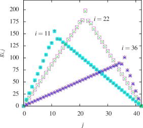
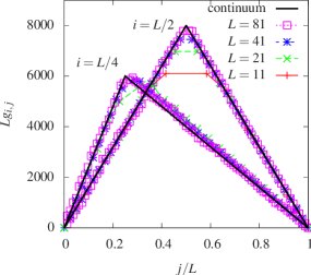
Figure 1: (a) Long-range part of the correlations, $g_{i,j}=C_{i,j}-2\delta_{ij}\kappa_{i}$, for an imposed temperature gradient and flat density profile, with $L=41$, $\rho=10$, $T_{0}=50$, $T_{L+1}=10$. Shown are the direct numerical results, using the numerical values of $C_{i,j}$ and $\kappa_{i}$, and the semi-analytical approximation obtained by solving numerically the discrete Poisson equation (3.8ilmnj) using the local equilibrium assumption $\kappa_{i}\simeq\rho_{i}/\beta^{2}$. In this and the following figures, each separate curve shows the stationary-state energy correlations $g_{i,j}$ for a given position $i$ as a function of $j$. (b) Rescaled correlations $Lg_{i,j}$ in the absence of a density gradient, as a function of $j/L$, $i=(L+1)/2$ and $i=(L+3)/4$, for the same parameter values as in (a) and different system sizes $L$. Onsite correlations $g_{i,i}$ are not shown. The exact result in the continuum limit is shown as a solid line.

The simplest case with non-trivial correlations is to impose a linear temperature gradient between two baths with temperatures $T_{0}\neq T_{L+1}$, but with a flat concentration gradient, i.e. $\rho_{0}=\rho_{L+1}=\rho$ for all $i$, and without bias in the dynamics ($p=q$). In this case, the density profile is flat throughout the system, $\rho_{i}=\rho$ for all $i$. The profile of mean energy is linear:

$$\left\langle E_{i}\right\rangle=\left\langle E_{0}\right\rangle+\frac{i}{L+1}\left(\left\langle E_{L+1}\right\rangle-\left\langle E_{0}\right\rangle\right).$$ (3.8ilmna)

Identifying as usual $T_{i}:=\left\langle E_{i}\right\rangle/\rho_{i}$, we can conclude that there is also a linear temperature profile under thse conditions; this is correctly obtained in simulations (not shown).

Figure 1 shows the long-range part of the energy correlations, $g_{i,j}$, in this case. Numerical results are compared to a numerical solution of the algebraic discrete Poisson equation (3.8ilmni). In order to carry out this numerical solution, the source terms $\kappa_{i}$ were assumed to take their local equilibrium value $\rho/\beta_{i}^{2}$, as described above. Despite this, we find very good agreement between the numerical results obtained from direct simulation and the numerical solution of the discrete diffusion equation. This holds everywhere, including for the onsite contribution of $g_{i,i}$.

Nonetheless, the agreement between the numerical and semi-analytical results is affected by the fact that the local thermodynamic equilibrium approximation is not strictly correct. As discussed in the introduction, the structure of the out-of-equilibrium measure is an open problem. However, here we can obtain an indication of the error in the local thermodynamic equilibrium approximation by comparing the value of $\kappa_{i}=\left\langle e_{i}^{2}/(m_{i}+1)\right\rangle$ obtained from a direct numerical average to the analytical value $\rho_{i}/\beta_{i}^{2}$ obtained from the local thermodynamic equilibrium assumption. This difference is shown in figure 2 for two different values of system size $L$. We see that the marginal distribution is not quite given by the local equilibrium approximation, but that it gets closer as $L$ increases, in agreement with the rigorous results of [23].

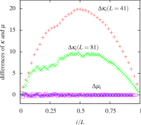
Figure 2: Difference $\Delta\kappa_{i}:=\kappa_{i}-\rho T_{i}^{2}$ of the value of $\kappa_{i}$ obtained from the direct numerical simulation and the analytical expression obtained with the local equilibrium assumption, for two values of system size $L$. The differences $\Delta\mu_{i}$ between the corresponding results for $\mu_{i}$ obtained by differenciation are also shown.

For the structure of the correlations $g_{i,j}$ away from the diagonal terms where $i=j$, the important quantities are the sources $\mu_{i}$, which are given by differences of the $\kappa_{i}$ as in (3.8ilmnk). The difference between the $\mu_{i}$ calculated by differentiating the numerically-obtained $\kappa_{i}$, and those obtained by differentiating the local equilibrium expression, are also shown in figure 2. They are very close to $0$, which is the reason for the excellent agreement between the numerical and semi-analytical results for the correlations.

In fact, this case (absence of concentration gradient) is simple enough to solve explicitly in the continuum limit. Taking $g(i,j)\to G(x,y)\,\delta x\,\delta y$, equation (3.8ilmnj) can be rewritten in the continuum limit as:

$$\frac{\partial G(x,y)}{\partial x^{2}}+\frac{\partial G(x,y)}{\partial y^{2}}=4c[T^{\prime}(x)]^{2}\,\delta(x-y),$$ (3.8ilmnb)

with boundary conditions $G(x=0,y)=G(x=L,y)=G(x,y=0)=G(x,y=L)=0$. The solution of this equation is readily found to be

$$G(x,y)=\frac{2c(\nabla T)^{2}}{L}\left\{\begin{array}[]{ll}x(L-y),&\mathrm{if\ }y>x\\ &\\ y(L-x),&\mathrm{if\ }y<x\end{array}\right..$$ (3.8ilmnc)

This result is similar to those of refs. [7, 11], but with the difference that the concentration $c$ now appears explicitly in the result.

As was pointed out in [16], the correlations for a system of size $L$ decay as $1/L$ if the boundary conditions are fixed (i.e. the values of the density and temperatures at the boundary are the same for diferent values of the system size $L$). Figure 1 shows the rescaled correlations $Lg_{i,j}$ for different system sizes compared to (3.8ilmnc). In the figure we have thus scaled space to the interval $[0,1]$ and rescaled the correlations by multiplying them by $L$. The various curves indeed converge to the limiting (continuum) form as $L\to\infty$. Note that the apparent $1/L$ scaling arises from the $\delta x$ term in the passage to the continuum limit: fixing the total system size and doubling the number of sites corresponds to halving $\delta x$.

5.3 Combined temperature gradient and concentration gradient

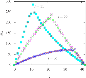
(a) $\rho_{0}=10$; $\rho_{L+1}=20$

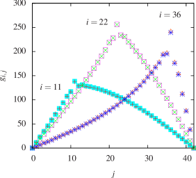
(b) $\rho_{0}=20$; $\rho_{L+1}=10$

Figure 3: Long-range part of the correlations, $g_{i,j}$, with imposed temperature and density gradients. The parameters are $L=41$, $T_{0}=50$, and $T_{L+1}=10$. The bath densities are $\rho_{0}=10$ and $\rho_{L+1}=20$ in (a), and are reversed in (b). The direct numerical and semi-analytical results again agree very well.

We now consider the effect of imposing both energy and concentration gradients, although still without bias in the motion ($p=q$). The profiles of $\rho_{i}$ and of $\left\langle E_{i}\right\rangle=\rho_{i}T_{i}$ are now both linear, so that $T_{i}=\left\langle E_{i}\right\rangle/\rho_{i}$ is a ratio of two linear functions, but is no longer itself linear.

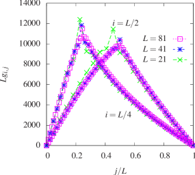
Figure 4: Scaling of correlations $Lg_{i,j}$, obtained from the semi-analytical solution, for different system sizes $L$, with parameters as in figure 3(a), for $i=(L+1)/2$ and $i=(L+3)/4$.

Figure 3 shows the numerical and semi-analytical results in this case. We find a skewing effect on the correlations, which is again in excellent agreement with the numerical results. The results are qualitatively very similar to those in [16], despite the differences in the nature of the models discussed in the introduction. Figure 4 shows the scaling of the correlations (obtained from the semi-analytical results) with system size. Again they converge to a continuum limit, corresponding to the solution of the continuous diffusion equation with sources given by (3.8ilmnv).

5.4 Effect of bias ($p\neq q$)

Upon introducing a bias in the directionality of the walkers’ jumps, that is by putting $p\neq q$, we obtain mean density and energy profiles which are no longer linear. Rather, they are given by [19]

$$\rho_{i} =\rho_{0}+\frac{1-\alpha^{i}}{1-\alpha^{L+1}}\,\left(\rho_{L+1}-\rho_{0}\right),$$ (3.8ilmnd)

$$\left\langle E_{i}\right\rangle =\left\langle E_{0}\right\rangle+\frac{1-\alpha^{i}}{1-\alpha^{L+1}}\,\left(\left\langle E_{L+1}\right\rangle-\left\langle E_{0}\right\rangle\right),$$ (3.8ilmne)

where $\alpha:=p/q$ and the quantities $\rho_{L+1}$, $\rho_{0}$, $\left\langle E_{L+1}\right\rangle$ and $\left\langle E_{0}\right\rangle$ are fixed by the boundary conditions.

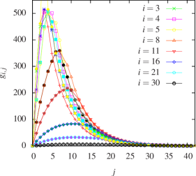
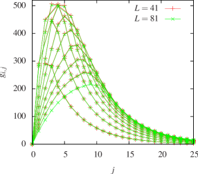
Figure 5: (a) Comparison of numerical and semi-analytical correlations $g_{i,j}$ for system size $L=41$, with parameters $\rho=10$, $T_{0}=50$, $T_{L+1}=5$, as a function of $j$, for $i=3$, $4$, $5$, $8$, $11$, $16$, $21$ and $30$ from top to bottom. There is a bias in the dynamics, with $p=0.35$ and $q=0.4$. (b) Comparison of the correlations for $L=41$ and $L=81$, with the same parameters as in (a). The numerical value of the correlations are the same for $i$ not too large. The lines are shown as a guide for the eye

Figure 5 shows the comparison between the numerically-obtained correlations and the semi-analytical solution, for a situation with a flat density profile (i.e. $\rho_{L+1}=\rho_{0}$), an imposed temperature gradient (which for constant density means that $\left\langle E_{L+1}\right\rangle\neq\left\langle E_{0}\right\rangle$) and a bias to the left. Again we find excellent agreement between the numerical results and the semi-analytical results. Note, however, that for values of $i$ around 30 and larger, the correlation function $g_{i,j}$ is very small for all values of $j$ ($j\neq i$). Hence, the energies at sites corresponding to large enough values of $i$ and $j$ are essentially uncorrelated. The reason for this is that, in the presence of a bias, the source of the correlations given in eq. (3.8ilmnv) decays exponentially as $i$ increases. Thus, in this case, since the bias is to the left, we expect the source of the correlations to be appreciable only up to distances of a few times the decay length $\lambda\sim 1/|\ln(\alpha)|$ (see eq. (3.8ilmne)) from the left boundary, and the effect of the right boundary to become negligible if the size of the system $L>>\lambda$. Indeed, figure 5 compares the correlations for two different system sizes with the same parameters. Clearly, the numerical values of the correlations are essentially independent of system size, and are negligible over a large part of the system.

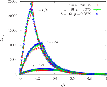
Figure 6: Rescaled semi-analytical correlations $Lg_{i,j}$ for biased dynamics as a function of $j/L$, for system sizes $L=41$, $L=81$ and $L=161$ and different $i$. In order to have a well-defined continuum limit, $q-p$ is halved when the system size is doubled, with $q=0.4$ fixed. Parameters are $\rho=10$, $T_{0}=50$, $T_{L+1}=5$.

Nonetheless, as was shown in section 3.2, it is possible to obtain a well-defined continuum limit for the energy correlations in the case of biased dynamics, provided the amount of bias changes in the correct way: the bias $q-p$ must be halved when the system size doubles, in addition to performing the same linear rescaling of space as in the other cases. Figure 6 confirms convergence to the continuum limit under these conditions.

6 Conclusions

By studying an extremely simple model of coupled transport of mass and a second conserved quantity, which we called energy, we have shown that the ubiquitous long-range correlations in this energy, whose transport depends on the motion of the mass, are present in the nonequilibrium stationary state, even though this quantity is completely passive. We were able to write down the equation describing the long-range spatial correlations for the energy in the system, and found that the structure of these correlations is remarkably similar to those found in more realistic models, as well as to the results of studies using fluctuating hydrodynamics. We thus conclude that the origin of these long-range correlations is already present in this simple model, and that a study of such models can go at least part of the way to explaining and quantifying the origin and structure of correlations in nonequilibrium systems. Nevertheless, we hope to be able to extend the methods and results to cases where the particle motion is modified by the energy carried by the particles.

Appendix A Derivation of energy partitioning distribution and entropy at a site

The distribution for the microcanonical partioning of energy among the particles at each site can be calculated as follows. First, given that the particles at each site are assumed to be in a state of microcanonical equilibrium, we can determine the probability that $l^{+}_{i}$ and $l^{-}_{i}$ out of the $m_{i}$ particles at site $i$ have combined energies $s^{+}_{i}$ and $s^{-}_{i}$ respectively, when the total energy at the site is $e_{i}$, as the quotient of the number of states consistent with these requirements over the total number of states available to the system. These numbers are proportional to the corresponding structure functions [24], given by

$$\omega(E,N,V):=\int\delta\left(H_{N}({\mathbf{p}},{\mathbf{q}})-E\right)\,{\mathrm{d}}{\mathbf{p}}\,{\mathrm{d}}{\mathbf{q}},$$ (3.8ilmna)

where $H_{N}({\mathbf{p}},{\mathbf{q}})$ is the $N$-particle Hamiltonian describing the dynamics at each site, and the integration is carried out over the phase space of the $N$ particles. If we assume that the particles are an ideal gas, then

$$H_{N}({\mathbf{p}},{\mathbf{q}})=\sum\limits_{j=1}^{N}\frac{|p_{i}|^{2}}{2m},$$ (3.8ilmnb)

where $m$ is the mass of the particles, and the required probability is given by

$$\mathbb{P}\left(\left.s^{+}_{i},s^{-}_{i}\right|l^{+}_{i},l^{-}_{i},m_{i},e_{i}\right)=$$ (3.8ilmnc)

$$\frac{\omega(s^{+}_{i},l^{+}_{i},V)\,\omega(s^{-}_{i},l^{-}_{i},V)\,\omega(e_{i}-s^{+}_{i}-s^{-}_{i},m_{i}-l^{+}_{i}-l^{-}_{i},V)}{\omega(e_{i},m_{i},V)}.$$ (3.8ilmnd)

For a $d$-dimensional ideal gas, we have

$$\omega(E,N,V)=\frac{(2\pi m)^{Nd/2}E^{Nd/2-1}V^{N}}{\Gamma(Nd/2)},$$ (3.8ilmne)

where $V$ is the volume accesible to the particles at each site, which we take as unity, and $\Gamma(\cdot)$ is the gamma function. Using this expression in (3.8ilmnc) yields

$$\mathbb{P}\left(\left.s^{+}_{i},s^{-}_{i}\right|l^{+}_{i},l^{-}_{i},m_{i},e_{i}\right)=$$ (3.8ilmnf)

$$\frac{\Gamma(m_{i}d/2)}{\Gamma(l^{+}_{i}d/2)\Gamma(l^{-}_{i}d/2)\Gamma([m_{i}-l^{+}_{i}-l^{-}_{i}]d/2)}\times$$ (3.8ilmng)

$$(s^{+}_{i})^{l^{+}_{i}d/2-1}(s^{-}_{i})^{l^{-}_{i}d/2-1}\frac{(e_{i}-s^{+}_{i}-s^{-}_{i})^{[m_{i}-l^{+}_{i}-l^{-}_{i}]d/2-1}}{e_{i}^{m_{i}d/2-1}},$$ (3.8ilmnh)

which, when $d=2$, simplifies somewhat, giving

$$\mathbb{P}\left(\left.s^{+}_{i},s^{-}_{i}\right|l^{+}_{i},l^{-}_{i},m_{i},e_{i}\right)=$$ (3.8ilmni)

$$\frac{\Gamma(m_{i})}{\Gamma(l^{+}_{i})\Gamma(l^{-}_{i})\Gamma(m_{i}-l^{+}_{i}-l^{-}_{i})}(s^{+}_{i})^{l^{+}_{i}-1}(s^{-}_{i})^{l^{-}_{i}-1}\frac{(e_{i}-s^{+}_{i}-s^{-}_{i})^{m_{i}-l^{+}_{i}-l^{-}_{i}-1}}{e_{i}^{m_{i}-1}}.$$ (3.8ilmnj)

Similarly, the classical entropy of the 2D gas at each site is given by [20]

$$S(e_{i},m_{i},V)=\ln[\omega(e_{i},m_{i},V)/m_{i}!]+m_{i}\sigma_{i}\sim m_{i}\ln[Ve_{i}/m_{i}^{2}]+m_{i}s_{i},$$ (3.8ilmnk)

taking the Boltzmann constant $k_{B}=1$, where $s_{i}$ and $\sigma_{i}$ are constants (i.e. they are independent of $e_{i}$, $m_{i}$ and $V$) which can vary from site to site.

References

References

- [1] Bonetto, F., Lebowitz, J. & Rey-Bellet, L. Fourier’s law: a challenge to theorists. In Fokas, A. S., Grigoryan, A., Kibble, T. & Zegarlinski, B. (eds.) Mathematical Physics 2000: Proceedings of the XIII International Congress on Mathematical Physics (Imperial College Press, London, 2000).
- [2] Lepri, S., Livi, R. & Politi, A. Thermal conduction in classical low-dimensional lattices. Phys. Rep. 377, 1–80 (2003).
- [3] Komatsu, T. S. & Nakagawa, N. Expression for the stationary distribution in nonequilibrium steady states. Phys. Rev. Lett. 100, 030601–4 (2008).
- [4] Evans, M. R., Majumdar, S. N. & Zia, R. K. P. Factorized steady states in mass transport models. J. Phys. A 37, L275–L280 (2004).
- [5] Dorfman, J. R., Kirkpatrick, T. R. & Sengers, J. V. Generic long-range correlations in molecular fluids. Ann. Rev. Phys. Chem. 45, 213–239 (1994).
- [6] de Zarate, J. M. O. & Sengers, J. V. Hydrodynamic Fluctuations in Fluids and Fluid Mixtures (Elsevier, Amsterdam, 2006).
- [7] Nicolis, G. & Mansour, M. M. Onset of spatial correlations in nonequilibrium systems: A master-equation description. Phys. Rev. A 29, 2845 (1984).
- [8] Kipnis, C., Marchioro, C. & Presutti, E. Heat flow in an exactly solvable model. J. Stat. Phys. 27, 65–74 (1982).
- [9] Spohn, H. Long range correlations for stochastic lattice gases in a non-equilibrium steady state. J. Phys. A 16, 4275–4291 (1983).
- [10] Garrido, P. L., Lebowitz, J. L., Maes, C. & Spohn, H. Long-range correlations for conservative dynamics. Phys. Rev. A 42, 1954+ (1990).
- [11] Suárez, A., Boon, J. P. & Grosfils, P. Long-range correlations in nonequilibrium systems: Lattice gas automaton approach. Phys. Rev. E 54, 1208+ (1996).
- [12] Derrida, B. Non-equilibrium steady states: fluctuations and large deviations of the density and of the current. J. Stat. Mech. Theor. Exp. 2007, P07023 (2007).
- [13] Delfini, L., Lepri, S., Livi, R. & Politi, A. Nonequilibrium invariant measure under heat flow. Phys. Rev. Lett. 101, 120604–4 (2008).
- [14] Lepri, S., Mejia-Monasterio, C. & Politi, A. A stochastic model of anomalous heat transport: analytical solution of the steady state. J. Phys. A 42, 025001 (2009).
- [15] Eckmann, J. P. & Young, L.-S. Nonequilibrium energy profiles for a class of 1-D models. Comm. Math. Phys. 262, 237–267 (2006).
- [16] Lin, K. & Young, L.-S. Correlations in nonequilibrium steady states of random halves models. J. Stat. Phys. 128, 607–639 (2007).
- [17] Mejía-Monasterio, C., Larralde, H. & Leyvraz, F. Coupled normal heat and matter transport in a simple model system. Phys. Rev. Lett. 86, 5417 (2001).
- [18] Larralde, H., Leyvraz, F. & Mejía-Monasterio, C. Transport properties of a modified Lorentz gas. J. Stat. Phys. 113, 197–231 (2003).
- [19] Antonio, A. M. R. & Larralde, H. The statistics of diffusive flux. J. Stat. Mech. Theor. Exp. 2005, P08012+ (2005).
- [20] Callen, H. B. Thermodynamics and an Introduction to Thermostatistics (Wiley, New York, 1985), 2nd edn.
- [21] Eckmann, J. P. & Young, L. S. Temperature profiles in Hamiltonian heat conduction. Europhys. Lett. 68, 790–796 (2004).
- [22] Groot, S. R. D. & Mazur, P. Non-Equilibrium Thermodynamics (Dover Publications, New York, 1984).
- [23] Ravishankar, K. & Young, L.-S. Local thermodynamic equilibrium for some stochastic models of Hamiltonian origin. J. Stat. Phys. 128, 641–665 (2007).
- [24] Reichl, L. E. A Modern Course in Statistical Physics (Wiley-Interscience, New York, 1998), 2nd edn.