Torsion cosmological dynamics

Abstract

In this paper, the dynamical attractor and heteroclinic orbit have been employed to make the late-time behaviors of the model insensitive to the initial condition and thus alleviate the fine-tuning problem in the torsion cosmology. The late-time de Sitter attractor indicates that torsion cosmology is an elegant scheme and the scalar torsion mode is an interesting geometric quantity for physics. The numerical solutions obtained by Nester et al. are not periodic solutions, but are quasi-periodic solutions near the focus for the coupled nonlinear equations.

I INTRODUCTION

The current observations, such as SNeIa (Supernovae type Ia), CMB (Cosmic Microwave Background) and large scale structure, converge on the fact that a spatially homogeneous and gravitationally repulsive energy component, referred as dark energy, accounts for about $70$ % of the energy density of universe. Some heuristic models that roughly describe the observable consequences of dark energy were proposed in recent years, a number of them stemming from a certain physics Padmanabhan01 and the others being purely phenomenological Copeland02 . About thirty years ago, the bouncing cosmological model with torsion was suggested in Ref.Kerlick , but the torsion was imagined as playing role only at high densities in the early universe. Goenner et al. made a general survey of the torsion cosmology Goenner , in which the equations for all the PGT (Poincaré Gauge Theory of gravity) cases were discussed although they only solved in detail a few particular cases. Recently some authors have begun to study torsion as a possible reason of the accelerating universe Boeheretal . Nester and collaborators shie03 consider an accounting for the accelerated universe in term of PGT: dynamic scalar torsion. With the usual assumptions of homogeneity and isotropy in cosmology, they find that torsion field could play a role of dark energy. This elegant model has only a few adjustable parameters, so scalar torsion may be easily falsified as ”dark energy”.

The fine-tuning problem should be one of the most important issues for the cosmological models, and a good model should limit the fine-tuning as much as possible. The dynamical attractor of the cosmological system has been employed to make the late-time behaviors of the model insensitive to the initial condition of the field and thus alleviates the fine-tuning problem Hao04 . In this paper, we study attractor and heteroclinic orbit in the torsion cosmology. We show that the late-time de Sitter behaviors cover a wide range of the parameters. This attractor indicates that torsion cosmology is an elegant scheme and the scalar torsion mode is an interesting geometric quantity for physics. Furthermore, there are only exact periodic solutions for the linearized system, which just correspond to the critical line (line of centers). The numerical solutions in Ref.shie03 are not periodic, but are quasi-periodic solutions near the focus for the coupled nonlinear equations.

II AUTONOMOUS EQUATIONS

PGT Hehl05 based on a Riemann-Cartan geometry, allows for dynamic torsion in addition to curvature. The affine connection of the Riemann-Cartan geometry is

$$\Gamma_{\mu\nu}{}^{\kappa}=\overline{\Gamma}_{\mu\nu}{}^{\kappa}+\frac{1}{2}(T_{\mu\nu}{}^{\kappa}+T^{\kappa}{}_{\mu\nu}+T^{\kappa}{}_{\nu\mu})\,,$$ (1)

where $\bar{\Gamma}_{\mu\nu}{}^{\kappa}$ is the Levi-Civita connection and $T_{\mu\nu}^{\kappa}$ is the torsion tensor. Meanwhile, the Ricci curvature and scalar curvature can be written as

$$R_{\mu\nu}=\overline{R}_{\mu\nu}+\overline{\nabla}_{\nu}T_{\mu}+\frac{1}{2}(\overline{\nabla}_{\kappa}-T_{\kappa})(T_{\nu\mu}{}^{\kappa}+T^{\kappa}{}_{\mu\nu}+T^{\kappa}{}_{\nu\mu})$$

$$+\frac{1}{4}(T_{\kappa\sigma\mu}T^{\kappa\sigma}{}_{\nu}+2T_{\nu\kappa\sigma}T^{\sigma\kappa}{}_{\mu})\,,$$ (2)

$$R=\overline{R}+2\overline{\nabla}_{\mu}T^{\mu}+\frac{1}{4}(T_{\mu\nu\kappa}T^{\mu\nu\kappa}+2T_{\mu\nu\kappa}T^{\kappa\nu\mu}-4T_{\mu}T^{\mu}),$$

where $\bar{R}_{\mu\nu}$ and $\bar{R}$ are the Riemannian Ricci curvature and scalar curvature, respectively, and $\bar{\nabla}$ is the covariant derivative with the Levi-Civita connection and $T_{\mu}\equiv T^{\nu}_{\mu\nu}$. According as Ref.shie03 we take the restricted form of torsion in this paper

$$T_{\mu\nu\rho}=\frac{2}{3}T_{[\mu}g_{\nu]\rho}$$ (4)

therefore, the gravitational Lagrangian density for the scalar mode is (For a detailed discussion see Ref.Nester2 )

$$L_{g} = -\frac{a_{0}}{2}R+\frac{b}{24}R^{2}$$ (5)

$$+\frac{a_{1}}{8}(T_{\nu\sigma\mu}T^{\nu\sigma\mu}+2T_{\nu\sigma\mu}T^{\mu\sigma\nu}-4T_{\mu}T^{\mu})\,,$$

Since current observations favor a flat universe, we will work in the spatially flat Robertson-Walker metric. According to the homogeneity and isotropy, the torsion $T_{\mu}$ should be only time dependent, so one can let $T_{t}(t)\equiv\Phi(t)$ and the spatial parts vanish since we have taken the restricted form (4) of torsion. For the general form, the torsion tensor have two independent components Goenner -Boeheretal . From the field equations one can finally give the necessary equations for the matter-dominated era to integrate (For a detailed discussion see Ref.shie03 )

$$\dot{H} = \frac{\mu}{6a_{1}}R-\frac{\rho}{6a_{1}}-2H^{2}\,,$$ (6)

$$\dot{\Phi} = -\frac{a_{0}}{2a_{1}}R-\frac{\rho}{2a_{1}}-3H\Phi+\frac{1}{3}\Phi^{2}\,,$$ (7)

$$\dot{R} = -\frac{2}{3}\left(R+\frac{6\mu}{b}\right)\Phi\,,$$ (8)

where $\mu=a_{1}-a_{0}$ and the energy density of matter component

$$\rho=\frac{b}{18}(R+\frac{6\mu}{b})(3H-\Phi)^{2}-\frac{b}{24}R^{2}-3a_{1}H^{2}\,.$$ (9)

One can scale the variables and the parameters as

$$t\rightarrow l_{p}^{-2}H_{0}^{-1}t,\,\,H\rightarrow l_{p}^{2}H_{0}H,\,\,\Phi\rightarrow l_{p}^{2}H_{0}\Phi,\,\,R\rightarrow l_{p}^{4}H_{0}^{2}R,$$

$$a_{0}\rightarrow l_{p}^{2}a_{0},\,\,a_{1}\rightarrow l_{p}^{2}a_{1},\,\,\mu\rightarrow l_{p}^{2}\mu,\,\,b\rightarrow l_{p}^{-2}H_{0}^{-2}b,$$ (10)

where $H_{0}$ is the present value of Hubble parameter and $l_{p}\equiv\sqrt{8\pi G}$ is the Planck length. Under the transform (10), Eqs. (6)-(8) remain unchanged. After transform, new variables $t$, $H$, $\Phi$ and $R$, and new parameters $a_{0}$, $a_{1}$, $\mu$ and $b$ are all dimensionless. Furthermore, the Newtonian limit requires $a_{0}=-1$. Obviously, Eqs. (6)-(8) is an autonomous system, so we can use the qualitative method of ordinary differential equations. It is worth noting that in the analysis of critical points, Copeland et al. Copeland introduced the elegant compact variables which are defined from the Friedmann equation constraint, but in our case, the Friedmann equation can not be written as the ordinary form, so the compact variables are not convenient here. Therefore, we will analyze the system of Eqs.(6)-(8) using the variables $H$, $\Phi$ and $R$ under the transform (10).

III LATE TIME DE SITTER ATTRACTOR

In the case of scalar torsion mode, the effective energy-momentum tensor can be represented as

$$\widetilde{T}_{t}{}^{t} = \!\!-3\mu H^{2}\!+\frac{b}{18}(R+\frac{6\mu}{b})(3H-\Phi)^{2}-\frac{b}{24}R^{2},$$ (11)

$$\widetilde{T}_{r}{}^{r} = \widetilde{T}_{\theta}{}^{\theta}=\widetilde{T}_{\phi}{}^{\phi}={1\over 3}[\mu(R-\overline{R})-\widetilde{T}_{t}{}^{t}]\,,$$ (12)

and the off-diagonal terms vanish. The effective energy density

$$\rho_{eff}=\rho+\rho_{T}\equiv\rho+\widetilde{T}_{tt},$$ (13)

which is deduced from general relativity. $p_{eff}=p_{T}\equiv\tilde{T}_{r}^{r}$ is an effective pressure, and the effective equation of state is

$$w_{eff}=\frac{\widetilde{T}_{r}^{r}}{\rho+\widetilde{T}_{tt}}$$ (14)

which is induced by the dynamic torsion.

According to equations (6)-(8), we can obtain the critical points and study the stability of these points. There are five critical points $(H_{c},\Phi_{c},R_{c})$ of the system as follows

$$(\text{i}) (0,0,0)$$ (15)

$$(\text{ii}) \scriptstyle\left(\left(\frac{3(1+a_{1})}{8}-A\right)\sqrt{B+C},\frac{3}{2}\sqrt{B+C},-\frac{6(1+a_{1})}{b}\right)$$

$$(\text{iii}) \scriptstyle\left(-\left(\frac{3(1+a_{1})}{8}-A\right)\sqrt{B+C},-\frac{3}{2}\sqrt{B+C},-\frac{6(1+a_{1})}{b}\right)$$

$$(\text{iv}) \scriptstyle\left(\left(\frac{3(1+a_{1})}{8}+A\right)\sqrt{B-C},\frac{3}{2}\sqrt{B-C},-\frac{6(1+a_{1})}{b}\right)$$

$$(\text{v}) \scriptstyle\left(-\left(\frac{3(1+a_{1})}{8}+A\right)\sqrt{B-C},-\frac{3}{2}\sqrt{B-C},-\frac{6(1+a_{1})}{b}\right)$$

where $A=\scriptstyle\frac{\sqrt{a_{1}^{2}(1+a_{1})^{3}(1+9a_{1})}}{8a_{1}(1+a_{1})}$, $B=\scriptstyle-\frac{(1+a_{1})(5+9a_{1})}{a_{1}b}$ and $C=\scriptstyle-\frac{3\sqrt{a_{1}^{2}(1+a_{1})^{3}(1+9a_{1})}}{a_{1}^{2}b}$. Consider that the parameter $b$ is associated with the quadratic scalar curvature term $R^{2}$, so that $b$ should be positive shie03 . Evidently, the critical points $(H_{c},\Phi_{c},R_{c})$ are not real values except (0, 0, 0) in the cases of parameters $b>0$ and $a_{1}>0$ or $-1\leq a_{1}<-1/9$.

If we consider the linearized equations, then Eqs. (6)-(8) are reduced to

$$\dot{H}=\frac{\mu}{6a_{1}}R,\qquad\dot{\Phi}=\frac{1}{2a_{1}}R,\qquad\dot{R}=-\frac{4\mu}{b}\Phi\,.$$ (16)

In the case $a_{1}>0$, there is only a critical point $(0,0,0)$ for the nonlinear system. Eqs. (16) has an exact periodic solution

$$H=\alpha R_{0}\sin\omega t+\frac{\mu}{3}\Phi_{0}\cos\omega t+H_{0}-\frac{\mu}{3}\Phi_{0},$$ (17)

$$\Phi=\beta^{-1}R_{0}\sin\omega t+\Phi_{0}\cos\omega t,$$ (18)

$$R=R_{0}\cos\ \omega t-\beta\Phi_{0}\sin\omega t,$$ (19)

where $\omega=\sqrt{\frac{2\mu}{a_{1}b}}$, $\alpha=\sqrt{\frac{b\mu}{72a_{1}}}$, $\beta=\sqrt{\frac{8\mu a_{1}}{b}}$ and $H_{0}=H(0)$, $\Phi_{0}=\Phi(0)$ and $R_{0}=R(0)$ are initial values. Obviously, ($H$, $0$, $0$) is a critical line for the linearized system. However, there is only a critical point $(0,0,0)$ for the nonlinear system which is an asymptotically stable focus. In other words, there is no periodic solution for the nonlinear system since the corresponding eigenvalue is ($0$, $-\sqrt{\frac{2\mu}{a_{1}b}}i$, $\sqrt{\frac{2\mu}{a_{1}b}}i$). In Fig.1, we plot the orbits near the point $(0,0,0)$ for the nonlinear systems.

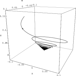
Figure 1: The phase diagrams of $(H,\Phi,R)$ for nonlinear system (6)-(8) with $a_{1}>0$. We take $a_{1}=0.9,b=8$ and the initial values $(0.8,0.5,1.1)$. $(0,0,0)$ is an asymptotically stable focus point.

Next, the parameters are restricted within $b>0$ and $-1/9\leq a_{1}<0$ or $a_{1}<-1$ in this paper. To study the stability of the critical points $(H_{c},\Phi_{c},R_{c})$, we write the variables near the critical points in the form $H=H_{c}+U$, $\Phi=\Phi_{c}+V$, and $R=R_{c}+X$ with $U,V,X$ the perturbations of the variables near the critical points. Substituting the expression into the system of equations (6)-(8), one can obtain the corresponding eigenvalues of critical points (i)-(v)

$$(\text{i})\scriptstyle(0,-\sqrt{-\frac{2(1+a_{1})}{a_{1}b}},\sqrt{-\frac{2(1+a_{1})}{a_{1}b}})$$

$$(\text{ii})\scriptstyle\left(-\sqrt{B+C},-3\left(\frac{3(1+a_{1})}{8}-A\right)\sqrt{B+C},-\left(\frac{1+9a_{1}}{8}-3A\right)\sqrt{B+C}\right)$$

$$(\text{iii})\scriptstyle\left(\sqrt{B+C},3\left(\frac{3(1+a_{1})}{8}-A\right)\sqrt{B+C},\left(\frac{1+9a_{1}}{8}-3A\right)\sqrt{B+C}\right)$$

$$(\text{iv})\scriptstyle\left(-\sqrt{B-C},-3\left(\frac{3(1+a_{1})}{8}+A\right)\sqrt{B-C},-\left(\frac{1+9a_{1}}{8}+3A\right)\sqrt{B-C}\right)$$

$$(\text{v})\scriptstyle\left(\sqrt{B-C},3\left(\frac{3(1+a_{1})}{8}+A\right)\sqrt{B-C},\left(\frac{1+9a_{1}}{8}+3A\right)\sqrt{B-C}\right)$$ (20)

The properties of the critical points are shown in tables 1 and 2. We find that critical point (ii) is a late time de Sitter attractor in the case of $-1/9\leq a_{1}<0$.

IV NUMERICAL ANALYSIS

In previous sections, we have studied the phase space of a torsion cosmology. The de Sitter attractor indicates that torsion cosmology Kerlick -shie03 is an elegant scheme and the scalar torsion mode is an interesting geometric quantity for physics. In this section, we study their dynamical evolution numerically.

Table 1: The physical properties of critical points for $a_{1}<-1$

critical points	property	$w_{eff}$	stability
(i)	focus	$\pm\infty$	stable
(ii)	saddle	-1	unstable
(iii)	saddle	-1	unstable
(iv)	saddle	-1	unstable
(v)	saddle	-1	unstable

The crossing of the $w=-1$ barrier is impossible in the traditional scalar field models Caldwell06 . The importance of the torsion cosmology is further promoted by this impossibility. In Fig. 2, we plot the dynamical evolution of the equation of state $w_{eff}$ for different initial values ($H$, $\Phi$, $R$). Contrary to the quintessence and phantom model Caldwell06 , the effective equation of state parameter $w_{eff}$ is dependent on time that can cross the cosmological constant divide $w_{\Lambda}=-1$ from $w_{eff}>-1$ to $w_{eff}<-1$ as the observations mildly indicate.

Critical points are always exact constant solutions in the context of autonomous dynamical systems. These points are often the extreme points of the orbits and therefore describe the asymptotic behavior. If the solutions interpolate between critical points they can be divided into a heteroclinic orbit and a homoclinic orbit (a closed loop). The heteroclinic orbit connects two different critical points and homoclinic orbit is an orbit connecting a critical point to itself. In the dynamical analysis of cosmology, the heteroclinic orbit is more interesting Li08 . If the numerical calculation is associated with the critical points, then we will find all kinds of heteroclinic orbits. Especially, the heteroclinic orbit is shown in Fig.3, which connects the positive and negative attractors.

Table 2: The physical properties of critical points for $-1/9\leq a_{1}<0$

critical points	property	$w_{eff}$	stability
(i)	saddle	$-\infty$	unstable
(ii)	positive attractor	-1	stable
(iii)	negative attractor	-1	unstable
(iv)	saddle	-1	unstable
(v)	saddle	-1	unstable

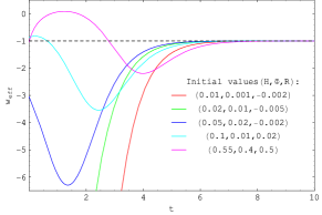
Figure 2: The evolution of the equation-of-state parameters $w_{eff}$ for different initial values$(H,\Phi,R)$ with $-1/9\leq a_{1}<0$. We take $a_{1}=-1/10,b=8$.

V CONCLUSION AND DISCUSSION

In this paper, we investigate the dynamics of a torsion cosmology, in which we consider only the ”scalar torsion” mode. This mode has certain distinctive and interesting qualities. We show that the late-time asymptotic behavior does not always correspond to an oscillating aspect. In fact, only in the focus case can we declare that ”scalar torsion” mode can contribute a quasinormal oscillating aspect to the expansion rate of the universe. There are only exact periodic solutions for the linearized system, which just correspond to the critical line (line of centers). Via numerical calculation of the coupled nonlinear equations Nester et al. shie03 plot that quasi-periodic solution near the focus.

The late-time de Sitter attractor indicates that torsion cosmology is an elegant scheme and the scalar torsion mode is an interesting geometric quantity for physics. We show that the late-time de Sitter behaviors cover a wide range of the parameters and thus alleviate the fine-tuning problem. Furthermore, the torsion cosmology has considered the possibility that the dynamics scalar torsion (geometric field) could fully account for the accelerated universe, which is naturally expected from spacetime gauge theory.

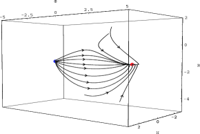
Figure 3: The phase diagrams of $(H,\Phi,R)$ with $-1/9\leq a_{1}<0$. The heteroclinic orbit connects the critical points case (iii) to case (ii). We take $a_{1}=-1/10,b=4$.

- (1) T. Padmanabhan, Phys. Rept. 380, 235 (2003); J. G. Hao and X. Z. Li, Phys. Rev. D67, 107303 (2003); D. J. Liu and X. Z. Li, Phys. Rev. D68, 067301 (2003); X. Z. Li and J. G. Hao, Phys. Rev. D69, 107303 (2004).
- (2) E. J. Copeland, M. Sami and S. Tsujikawa, Int. J. Mod. Phys. D15, 1753 (2006); J. G. Hao and X. Z. Li, Phys. Lett. B606, 7 (2005); D. J. Liu and X. Z. Li, Phys. Lett. B611, 8 (2005); D. J. Liu, C. B. Sun and X. Z. Li, Phys. Lett. B634, 442 (2006).
- (3) G. D. Kerlick, Ann. Phys. 99, 127 (1976)
- (4) H. Goenner and F. Müller-Hoissen, Class. Quant. Grav. 1, 651 (1984)
- (5) S. Capozziello, S. Carloni and A. Troisi, Recent Res. Dev. Astron. Astrophys. 1, 625 (2003); C. G. Böhmer, J. Burnett, Phys. Rev. D78, 104001 (2008); C. G. Böhmer, Acta Phys. Polon. B36, 2841 (2005); E. W. Mielke and E. SanchezRomero, Phys. Rev. D73, 043521 (2006); A. V. Minkevich, A. S. Garkin and V. I. Kudin, Class. Quant. Grav. 24, 5835 (2007)
- (6) K. F. Shie, J. M. Nester and H. J. Yo, Phys. Rev. D78, 023522 (2008); H. J. Yo and J. M. Nester, Mod. Phys. Lett. A22, 2057 (2007).
- (7) J. G. Hao and X. Z. Li, Phys. Rev. D70, 043529 (2004).
- (8) F. W. Hehl, J. D. McCrea, E. W. Mielke and Y. Neeman, Phys. Rept. 258, 1 (1995); M. Blagojević, Gravitation and Gauge Symmetries (Institute of Physics, Bristol, 2002); T. Ortín, Gravity and strings, (Cambridge University Press, Cambridge, 2004).
- (9) H. J. Yo and J. M. Nester, Int. J. Mod. Phys. D8, 459 (1999).
- (10) E. J. Copeland, A. R. Liddle and D. Wands, Phys. Rev. D57, 4686 (1998)
- (11) R. R. Caldwell and M. Doran, Phys. Rev. D72, 043527 (2005); J. G. Hao and X. Z. Li, Phys. Rev. D68, 083514 (2003).
- (12) X. Z. Li, Y. B. Zhao and C. B. Sun, Class. Quant. Grav. 22, 3759 (2005).