Viscous Cardassian universe

Abstract

The viscous Cardassian cosmology is discussed, assuming that there is a bulk viscosity in the cosmic fluid. The dynamical analysis indicates that there exists a singular curve in the phase diagram of viscous Cardassian model. In the viscous PL model, the equation-of-state parameter $w_{k}$ is no longer a constant and it can cross the cosmological constant divide $w_{\Lambda}=-1$, in contrast with same problem of the ordinary PL model. Other models possess with similar characteristics. For MP and exp models, $w_{k}$ evolves more near $-1$ than the case without viscosity. The bulk viscosity also effect the virialization process of a collapse system in the universe: $\frac{R_{vir}}{R_{ta}}$ is increasingly large when the bulk viscosity is increasing. In other words, the bulk viscosity retards the progress of collapse system. In addition, we fit the viscous Cardassian models to current type Ia supernovae data and give the best fit value of the model parameters including the bulk viscosity coefficient $\tau$.

Managing Editor

1 Introduction

The current accelerating expansion of the universe indicated by the astronomical measurements from high redshift supernovae[1] as well as accordance with other observations such as the Boomerang/Maxima/WMAP data[2] and galaxy power spectra[3] becomes one of the biggest puzzles in the research field of cosmology. One popular theoretical explanation approach is to assume that there exists a mysterious energy component, dubbed dark energy, with negative pressure, or equation of state with $w=p/\rho<0$ that currently dominates the dynamics of the universe(see[4] and references therein). Such a component makes up $70\%$ of the energy density of the universe yet remains elusive in the context of general relativity and the standard model of particle physics. The most natural dark energy candidate is a cosmological constant which arises as the result of a combination of general relativity(GR) and quantum field theory. However, its theoretical value is between $60-120$ orders of magnitude higher than the observed value. An alternative candidate is a slowly evolving and spatially homogeneous scalar field, referred to as ”quintessence” with $w>-1$[4] and ”phantom” with $w<-1$[5], respectively. Since current observational constraint on the equation of state of dark energy lies in a relatively large around the so-called cosmological constant divide $w_{\Lambda}=-1$, it is still too early to rule out any of the above candidates. However, the expectation of explaining cosmological observations without requiring new energy component is undoubtedly worth of investigation. GR is very well examined in the solar system, in observation of the period of the binary pulsar, and in the early universe, via primordial nucleosynthesis, but no one has so far tested in the ultra-large length scales and low curvatures characteristic of the Hubble radius today. Therefore, it is a priori believable that Friedmann equation is modified in the very far infrared, in such a way that the universe begins to accelerate at late time. Freese and Lewis[6] construct so-called Cardassian universe models that incarnates this hope. The Cardassian universe is a proposed modification to the Friedmann equation in which the universe is flat and accelerating, and yet contains only matter(baryonic or not) and radiation. But the ordinary Friedmann equation governing the expansion of the universe is modified to be

$$H^{2}\equiv\left(\frac{\dot{a}}{a}\right)^{2}=\frac{8\pi G}{3}g(\rho)$$ (1)

where $\rho$ consists only of matter and radiation, $H$ is the Hubble ”parameter” which is a function of time, $a$ is the scale factor of the universe, and $G=1/m_{pl}^{2}\equiv\frac{\kappa^{2}}{8\pi}$ is the Newtonian gravitational constant. Note that as required by inflation scenario and observations of CMB, the geometry of the universe is flat, therefore, there are no curvature terms in the above equation. The function $g(\rho)$ returns to ordinary Friedmann equation at early times, but that takes a distinct form that drives an accelerated expansion in the recent past of the universe at $z<\mathcal{O}(1)$. In Cardassian models, we simply set the cosmological constant $\Lambda=0$, and the only compositions are matter and radiation. A possible interpretation of Cardassian arose from consideration of braneworld scenarios, in which our observable universe is a 3-dimensional brane embedded in a higher dimensional universe. An alternative interpretation had been also discussed[8], in which one developed a 4-dimensional fluid description of Cardassian cosmology. The observational constraints of Cardassian models have been extensively studied[9]. The simplest model is power law Cardassian modle(PL) with an additional term $\rho^{n}$, which satisfies many observational constrains: the first Doppler peak of CMB is slightly shifted, the universe is rather older, and the early structure formation($z>1$) is unaffected. Furthermore, one can consider other forms of $g(\rho)$ including the modified polytropic model(MP) and the exponential model(exp)

$$g(\rho)=\left\{\begin{array}[]{ll}\rho\left[1+\left(\frac{\rho}{\rho_{card}}\right)^{n-1}\right],&\textrm{for PL}\\ \rho\left[1+\left(\frac{\rho_{card}}{\rho}\right)^{qn}\right]^{\frac{1}{q}},&\textrm{for MP}\\ \rho\exp\left[\left(\frac{\rho_{card}}{\rho}\right)^{n}\right],&\textrm{for exp}\end{array}\right.$$ (5)

where $\rho_{card}$ is a characteristic constant energy density and $q$ and $n$ are two dimensionless positive constants[10]. Obviously, at early times, $\rho$ is much larger than the characteristic energy density $\rho_{card}$, $g(\rho)\rightarrow\rho$, i.e. Eq.(1) recovers the ordinary Friedmann equation.

On the other hand, the dissipative effects, including both bulk and shear viscosity, are supposed to play a very important role in the astrophysics (see Ref.astro viscous and references therein) and the nuclear physics (see Ref.nucl viscous and references therein). Under the conditions of spatial homogeneity and isotropy, a scalar bulk viscous pressure is the solely admissible dissipative phenomenon. The viscosity theory of relativistic fluids was first suggested by Eckart[13] and Landau and Lifshitz[14], who considered only first-order deviation from equilibrium, which leads to parabolic differential equations and hence to an infinite speed of propagation for heat flow and viscosity, in contradiction with the principle of causality. The relativistic second-order theory was founded by Israel[15], and has also been used in the evolution of the universe[16]. However, the character of the evolution equation is very complicated in the framework of the full causal theory. Therefore, the conventional theory[14] is still applied to phenomena which are quasi-stationary, i.e., slowly varying on space and time scales characterized by the mean free path and the mean collision time. In the case of isotropic and homogeneous cosmologies, the dissipative process can be modelled as a bulk viscosity $\zeta$ within a thermodynamical approach. Some original works on the bulk viscous cosmology were done by Belinsky and Khalatnikov[17]. The bulk viscosity introduces dissipation by only redefining the effective pressure, $p_{eff}$, according to $p_{eff}=p-3\zeta H$ where $H$ is the Hubble parameter. The condition $\zeta>0$ assures a positive entropy production in conformity with the second law of thermodynamics[18]. We are interested in two solvable cases: (i) $\zeta=\sqrt{3}\kappa^{-1}\tau H$, where $\tau$ is a constant. This assumption implicates that $\zeta$ is directly proportional to the divergence of the cosmic fluid’s velocity vector. Therefore, it is physically natural, and has been considered previously in an astrophysical context[19]; (ii) $\zeta=\tau\left(g(\rho)\right)^{\alpha+\frac{3}{2}}$. This dependence is more complicated, but one can see in the following some interesting results obtained. Obviously, case (i) is equivalent to one with $\alpha=-1$ of case (ii).

In this paper, we consider a viscous Cardassian cosmological model for the expanding universe, assuming that there is bulk viscosity in the cosmic fluid. The dynamical analysis indicates that there exists a singular curve in the phase diagram for various models. The numerical result show that $\frac{R_{vir}}{R_{ta}}$ is increasingly large when the bulk viscosity is increasing. Furthermore, we fit the viscous Cardassian models to current SNeIa data and give the best fit values of the parameters including the bulk viscosity coefficient $\tau$.

2 The model

In the viscous Cardassian model, the modified Friedmann equation is described by Eq.(1). For the late-time evolution of the universe we neglect the contribution of radiation, so that Eq.(1) is reduced to

$$H^{2}=\frac{\kappa^{2}}{3}g(\rho_{m})$$ (6)

where $\rho_{m}$ is the energy density of matter, which keeps conserved during the expansion of the universe, i.e.,

$$\dot{\rho}_{m}+3H(\rho_{m}-3H\zeta_{m})=0$$ (7)

where $\zeta_{m}$ is the bulk viscosity for the matter energy density $\rho_{m}$. In the $\zeta_{m}=0$ case, the evolution of matter takes the ordinary manner $\rho_{m}=\rho_{m,0}(1+z)^{3}$ where $\rho_{m,0}$ is the present value of energy density of matter. However, the evolution of matter is not likely power law of $(1+z)$ in the $\zeta_{m}\neq 0$ case. Similarly, the conservation equation of total energy density can be written as

$$\dot{g}(\rho_{m})+3H\left[g(\rho_{m})+p-3H\zeta\right]=0$$ (8)

where $\zeta$ is the bulk viscosity for total energy density $g(\rho_{m})$. Combing Eqs.(7) and (8), it is easy to check that $\zeta=\frac{\partial g(\rho_{m})}{\partial\rho_{m}}\zeta_{m}$. Following Ref.P.Gondolo, we take the energy density to be the sum of two terms:

$$g(\rho_{m})=\rho_{m}+\rho_{k}$$ (9)

where $\rho_{k}$ is a Cardassian contribution. The thermodynamics of an adiabatically expanding universe tell us that pressure of Cardassian contribution is

$$p_{k}=\rho_{m}\frac{\partial g(\rho_{m})}{\partial\rho_{m}}-g(\rho_{m}),$$ (10)

and $p=p_{k}$ because of $p_{m}=0$. From Eqs.(9) and (10), we have the equation of state

$$w_{k}=\frac{p_{k}-3H\zeta}{g(\rho_{m})-\rho_{m}}.$$ (11)

Furthermore, we have

$$\dot{H}+H^{2}=\frac{\ddot{a}}{a}=-\frac{\kappa^{2}}{6}\left[g(\rho_{m})+3(p_{k}-3H\zeta)\right]$$ (12)

which is the acceleration equation of the cosmological expansion. Using Eqs.(6),(8) and (10), we obtain

$$a\frac{dg(\rho_{m})}{da}+3\rho_{m}\frac{dg(\rho_{m})}{d\rho_{m}}-3\kappa\sqrt{3g(\rho_{m})}\zeta=0.$$ (13)

We shall be interested in the evolution of the late universe, from $t=t_{0}$ onwards, where $t_{0}$ is the initial time and the corresponding scale factor $a(t_{0})=a_{0}$ and energy density $\rho_{m}(t_{0})=\rho_{m,0}$. From Eq.(13), we have

$$a=a_{0}\left(\exp\left[\int_{\rho_{m,0}}^{\rho_{m}}\frac{dg(\rho_{m})}{3\kappa\sqrt{3g(\rho_{m})}\zeta-3\rho_{m}\frac{dg(\rho_{m})}{d\rho_{m}}}\right]\right)$$ (14)

which is the general relation between the cosmological scale factor $a$ and the energy density $\rho_{m}$.

In what follows, we focus on the viscous Cardassian model, as the cosmological dynamics are analytically solvable when we choose $\zeta=\sqrt{3}\kappa^{-1}\tau H$ where $\tau$ is a constant. The scale factor is given by

$$\frac{a}{a_{0}}=\frac{f(\Omega_{m})}{f(\Omega_{m,0})}$$ (15)

where $\Omega_{m}$ is the density parameter of matter and $\Omega_{m,0}$ is the present value of $\Omega_{m}$. For the PL model, we have

$$f(\Omega_{m})=\left[\frac{\Omega_{m}^{(\sqrt{3}\kappa\tau-1)n}(\Omega_{m}-1)^{n-\sqrt{3}\kappa\tau}}{[n(\Omega_{m}-1)-\Omega_{m}+\sqrt{3}\kappa\tau]^{\sqrt{3}\kappa\tau(n-1)}}\right]^{\frac{1}{3(n-1)(n-\sqrt{3}\kappa\tau)(\sqrt{3}\kappa\tau-1)}}$$ (16)

and the equation of state

$$w_{k}=\frac{(1-n)(\Omega_{m}-1)-\sqrt{3}\kappa\tau}{1-\Omega_{m}}.$$ (17)

In the late time of universe, the new term of PL model is so large that the ordinary first term $\rho_{m}$ can be neglected. In other words, we have $\Omega_{m}\ll 1$, so that the expansion is superluminal (accelerated) for $n<\frac{2}{3}+\sqrt{3}\kappa\tau$.

For the MP model, we have

$$f(\Omega_{m})=\left[\frac{\Omega_{m}^{q(\sqrt{3}\kappa\tau-1)(n-1)}(\Omega_{m}^{q}-1)^{n+\sqrt{3}\kappa\tau-1}}{(\sqrt{3}\kappa\tau+n-1-n\Omega_{m}^{q})^{\sqrt{3}\kappa\tau n}}\right]^{\frac{1}{3qn(1-\sqrt{3}\kappa\tau)(\sqrt{3}\kappa\tau+n-1)}}$$ (18)

and

$$w_{k}=\frac{n(\Omega_{m}^{q}-1)-\sqrt{3}\kappa\tau}{1-\Omega_{m}}.$$ (19)

For the exp model, we have

$$f(\Omega_{m})=\left[\frac{\ln\Omega_{m}}{(1-\sqrt{3}\kappa\tau+n\ln\Omega_{m})^{\sqrt{3}\kappa\tau}}\right]^{\frac{1}{3n(1-\sqrt{3}\kappa\tau)}}$$ (20)

and

$$w_{k}=\frac{n\ln\Omega_{m}-\sqrt{3}\kappa\tau}{1-\Omega_{m}}.$$ (21)

We plot the evolution of $w_{k}$ for different values of $\kappa\tau$ in Fig. 1. As can be seen, in viscous PL model, $w_{k}$ is no longer a constant and it is dependent on time that can cross the cosmological constant divide $w_{\Lambda}=-1$. For MP and exp models, $w_{k}$ evolves more near $-1$ than the case without viscosity.

In the $\tau=0$ case, Eqs.(16) -(21) reduce to the results of ordinary Cardassian model without viscosity and Eq.(15) is solvable for the three models:

$$\Omega_{m}=\left\{\begin{array}[]{ll}\frac{\frac{\Omega_{m,0}}{1-\Omega_{m,0}}(1+z)^{3(1-n)}}{1+\frac{\Omega_{m,0}}{1-\Omega_{m,0}}(1+z)^{3(1-n)}},&\textrm{for PL}\\ \left[\frac{\frac{\Omega_{m,0}^{q}}{1-\Omega_{m,0}^{q}}(1+z)^{3qn}}{1+\frac{\Omega_{m,0}^{q}}{1-\Omega_{m,0}^{q}}(1+z)^{3qn}}\right]^{\frac{1}{q}},&\textrm{for MP}\\ \\ \Omega_{m,0}^{(1+z)^{-3n}}.&\textrm{for exp}\end{array}\right.$$ (26)

Figure 1: In the $\zeta=\sqrt{3}\kappa^{-1}\tau H$ case, the evolution of the equation-of-state parameters $w_{k}$ for different values of $\kappa\tau$.

3 Autonomous system

A general study of the phase space system of quintessence and phantom in FRW universe has been given in Ref.phase space system. For the viscous Cardassian cosmological dynamical system, the corresponding equations of motion can be written as

$$\dot{H}=-\frac{\kappa^{2}}{2}\left(\rho_{m}\frac{dg(\rho_{m})}{d\rho_{m}}-3H\zeta\right),$$ (27)

$$\dot{\rho_{m}}+3H\left(\rho_{m}-3H\zeta\frac{d\rho_{m}}{dg(\rho_{m})}\right)=0$$ (28)

and Eq.(6). To analyze the dynamical system, we rewrite the equations with the following dimensionless variables: $x=\frac{\kappa^{2}\rho_{m}}{3H^{2}}$,$y=\frac{\kappa^{2}\zeta}{3H}$,$z=\frac{dg(\rho_{m})}{d\rho_{m}}$ and $N=\ln a$. The dynamical system can be reduced to

$$\frac{dx}{dN}=\frac{9y}{z}-3x+3x^{2}z-9xy,$$ (29)

$$\frac{dy}{dN}=u+\frac{3}{2}xyz-\frac{9}{2}y^{2},$$ (30)

where $z$ and $u$ are both functions of $x$ and $y$. $z(x,y)$ is determined by the specified form of $g(\rho_{m})$ and $u\equiv\frac{\kappa^{2}}{3H^{2}}\frac{\partial\zeta}{\partial N}$ is determined by the specified form of viscosity. The equation of state can be expressed in terms of the new variables as

$$w_{k}=\frac{xz-3y-1}{1-x}$$ (31)

and the sound speed is

$$c_{s}^{2}=\left\{\begin{array}[]{ll}\frac{n(n-1)(1-x)}{n+(1-n)x},&\textrm{for PL}\\ \frac{n(1-x^{q})\left[n-1+(q-1)nx^{q}\right]}{nx^{q}+1-n},&\textrm{for MP}\\ \frac{n(1-n)\ln x+n^{2}(\ln x)^{2}}{1+n\ln x},&\textrm{for exp.}\end{array}\right.$$ (35)

We choose $\zeta=\tau\left(g(\rho)\right)^{\alpha+\frac{3}{2}}$ and show the critical points of the autonomous systems and their properties in Table 3. In Fig. 2, the phase diagrams of the three models are given, respectively. It is worth noting that there exists a singular curve (bold line) in the viscous Cardassian’s phase diagrams.

The critical points and their properties in the $\zeta=\tau(g(\rho_{m}))^{\alpha+\frac{3}{2}}$ case. Critical points$\scriptstyle(x,y)$ Eigenvalues Stability         PL model $\scriptstyle(0,0)$ $\left(\scriptstyle 3(n-1),\scriptstyle-3n(1+\alpha)\right)$ $\left\{\begin{array}[]{ll}\scriptstyle 0<n<\frac{2}{3},\alpha>-1\\ \textrm{\scriptsize or}\scriptstyle\quad n<0,\alpha<-1\end{array}\right.$,stable $\scriptstyle(1,0)$ $\left(\scriptstyle 3(1-n),-3(1+\alpha)\right)$ unstable $\scriptstyle\left(x_{0},\scriptstyle\frac{(1-n)x_{0}+n}{3}\right)$ $\left(\scriptstyle 0,\scriptscriptstyle 3\left[(1-n)(2+\alpha)x_{0}+(1+\alpha)n-1+\frac{n}{n+(1-n)x_{0}}\right]\right)$ $\left\{\begin{array}[]{ll}\scriptscriptstyle\frac{x_{0}}{x_{0}-1}<n<\frac{2}{3},\alpha<\frac{[1-4n+3n^{2}-2(1-n)^{2}x_{0}]x_{0}-n^{2}}{[n+(1-n)x_{0}]^{2}}\\ \textrm{\scriptsize or}\scriptscriptstyle n<\frac{x_{0}}{x_{0}-1},\alpha>\frac{[1-4n+3n^{2}-2(1-n)^{2}x_{0}]x_{0}-n^{2}}{[n+(1-n)x_{0}]^{2}}\end{array}\right.$stable         MP model $\scriptstyle(1,0)$ $\scriptstyle(-3(1+\alpha),3qn)$ unstable $\scriptstyle\left(\left(\frac{n-1}{n}\right)^{\frac{1}{q}},0\right)$ $\scriptstyle(0,3q(n-1)-3)$ $\left\{\begin{array}[]{ll}\scriptstyle q(n-1)<1,&\textrm{\scriptsize stable}\\ \scriptstyle q(n-1)>1,&\textrm{\scriptsize unstable}\end{array}\right.$ $\scriptstyle(x_{0},\scriptstyle\frac{1-n+nx_{0}^{q}}{3})$ $\left(\scriptstyle 0,\scriptscriptstyle 3\left[(1+\alpha)(1-n)+(1+q+\alpha)nx_{0}^{q}-\frac{qnx_{0}^{q}}{1-n+nx_{0}^{q}}\right]\right)$ $\left\{\begin{array}[]{ll}\scriptscriptstyle(1+\alpha)(1-n)+(1+n+\alpha)nx_{0}^{q}<\frac{nqx_{0}^{q}}{1-n+nx_{0}^{q}}\\ \textrm{\scriptsize and}\scriptscriptstyle\quad 1-n+nx_{0}^{q}\neq 0\end{array}\right.$,stable         exp model $\scriptstyle(1,0)$ $\scriptstyle(3n,-3(1+\alpha))$ unstable $\scriptstyle(e^{-\frac{1}{n}},0)$ $\scriptstyle(0,3(n-1))$ $\left\{\begin{array}[]{ll}\scriptstyle 0<n<1,&\textrm{\scriptsize stable}\\ \scriptstyle n>1,&\textrm{\scriptsize unstable}\end{array}\right.$ $\scriptstyle\left(x_{0},\scriptstyle\frac{1+n\ln x_{0}}{3}\right)$ $\left(\scriptstyle 0,\scriptstyle 3\left[1+\alpha+n+n(1+\alpha)\ln x_{0}-\frac{n}{1+n\ln x_{0}}\right]\right)$ $\left\{\begin{array}[]{ll}\scriptstyle 1+\alpha+n+n(1+\alpha)\ln x_{0}<\frac{n}{1+n\ln x_{0}}\\ \textrm{\scriptsize and}\scriptstyle\quad 1+n\ln x_{0}\neq 0\end{array}\right.$,stable

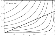
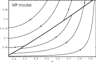
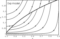
Figure 2: In the $\zeta=\tau\left(g(\rho)\right)^{\alpha+\frac{3}{2}}$ case, the phase diagrams of $(x,y)$ for PL, MP and exp models. There is a singular curve (bold line) which formed of critical points in the phase diagrams. We choose the parameters to be $n=-0.01,\alpha=0.2$ for PL, $q=1.15,n=1.1,\alpha=1.5$ for MP and $n=0.8,\alpha=2.5$ for exp, respectively.

4 Virialization

The spherical collapse formalism developed by Gunn and Gott[21] is a simple but powerful tool for studying the growth of inhomogeneities and bound systems in the universe. It describes how an initial inhomogeneity decouples from the expansion of the universe and then expands slower, eventually reaches the state of turnaround and collapses. Physically we assumes that the collapse system goes through a virialization process and stabilizes at a finite size. An important parameter of the spherical collapse model is the ratio between the virialized radius and the turnaround radius $\frac{R_{vir}}{R_{ta}}$[22].

Using energy conservation between virialization and turnaround, one can get

$$\left[U+T\right]_{vir}=U_{ta}$$ (36)

where $U$ is the potential energy, $T=\frac{R}{2}\frac{\partial U}{\partial R}$ is the kinetic energy of the system. If the collapse object is made up of only one energy component, the potential and the potential energy within it are

$$\Phi(r)=-2\pi G(1+3w)\rho\left(R^{2}-\frac{r^{2}}{3}\right)$$ (37)

and

$$U=\frac{1}{2}\int\rho\Phi dV$$ (38)

where $R$ is the radius of the spherical collapse system. In the Einstein-de Sitter universe, for a spherical perturbation with conserved mass $M$, $\Phi(r)=\frac{GM}{2R^{3}}(r^{2}-3R^{2})$, $U=-\frac{3GM^{2}}{5R}$, $T_{vir}=-\frac{U}{2}$, and the ratio of virialization to turnaround is $\frac{R_{vir}}{R_{ta}}=\frac{1}{2}$.

In the PL model without bulk viscosity, we have

$$\Phi=-2G\pi\rho_{m}\left(R^{2}-\frac{r^{2}}{3}\right)\left[1+\left(\frac{\rho_{m}}{\rho_{card}}\right)^{n-1}\right]\left\{1+3\left[n-1+\frac{(1-n)\rho_{m}}{\rho_{m}+\rho_{card}\left(\frac{\rho_{m}}{\rho_{card}}\right)^{n}}\right]\right\}$$

and

$$U=-\frac{16}{15}G\pi^{2}R^{5}\left[\rho_{m}+\rho_{card}\left(\frac{\rho_{m}}{\rho_{card}}\right)^{n}\right]\left[\rho_{m}+(3n-2)\rho_{card}\left(\frac{\rho_{m}}{\rho_{card}}\right)^{n}\right]\;.$$

Using the relation $\rho_{m,vir}=\rho_{m,ta}\xi^{-3}$ where $\xi\equiv\frac{R_{vir}}{R_{ta}}$, Eq.(36) can be written as

$$\left\{2\xi\left[1+(1+z_{ta})^{3n-3}(\Omega_{m,0}^{-1}-1)\right]\left[(3n-2)(1+z_{ta})^{3n-3}(\Omega_{m,0}^{-1}-1)+1\right]-1\right\}\xi^{6n}+$$

$$(9n^{2}-15n+4)(1+z_{ta})^{3n-3}(\Omega_{m,0}^{-1}-1)\xi^{3+3n}+(3n-2)(6n-7)(1+z_{ta})^{6n-6}(\Omega_{m,0}^{-1}-1)^{2}\xi^{6}$$

$$=0\;.$$ (41)

It is difficult to find analytical solution for Eq.(4), therefore we have to investigate it numerically. The result is shown in Fig. 3 (solid line). In the viscous PL model with $\zeta=\sqrt{3}\kappa^{-1}\tau H$, same problem becomes more complex. As the function of scale factor $a$, $\rho_{m}$ is determined by

$$\left[\sqrt{3}\kappa\tau\left(1+\left(\frac{\rho_{card}}{\rho_{m,0}}\right)^{1-n}\right)-1-n\left(\frac{\rho_{card}}{\rho_{m,0}}\right)^{1-n}\right]\left(\frac{a}{a_{0}}\right)^{\frac{3(\sqrt{3}\kappa\tau-1)(\sqrt{3}\kappa\tau-n)}{\sqrt{3}\kappa\tau}}$$ (42)

$$=(\sqrt{3}\kappa\tau-1)\left(\frac{\rho_{m}}{\rho_{m,0}}\right)^{1-\frac{n}{\sqrt{3}\kappa\tau}}+(\sqrt{3}\kappa\tau-n)\left(\frac{\rho_{card}}{\rho_{m,0}}\right)^{1-n}\left(\frac{\rho_{m}}{\rho_{m,0}}\right)^{n-\frac{n}{\sqrt{3}\kappa\tau}}.$$

Combing (42) and (36), we obtain the relation between $\xi$ and turnaround redshift $z_{ta}$. In Fig. 3, we show $\xi$ as a function of $z_{ta}$ for different bulk viscosity coefficients. As can be seen, in Cardassian models, the ratio $\frac{R_{vir}}{R_{ta}}$ is always larger than $\frac{1}{2}$, and it get larger and larger with the evolution of the universe. It means that collapse process will be harder and harder to occur ($\xi\rightarrow 1$). Furthermore, $\xi$ becomes larger when $\tau$ takes larger value.

Figure 3: In the viscous PL model with $\zeta=\sqrt{3}\kappa^{-1}\tau H$, $\xi$ as a function of $z_{ta}$ for different bulk viscosity coefficients $\tau$.

5 Fit the model parameters to supernovae data

In general, the approach towards determining the expansion history $H(z)$ is to assume an arbitrary ansatz for $H(z)$ which is not necessarily physically motivated but is specially designed to give a good fit to the data for $d_{L}(z)$. Given a particular cosmological model for $H(z;a_{1},...,a_{n})$ where $a_{1},...,a_{n}$ are model parameters, the maximum likelihood technique can be used to determine the best fit values of parameters as well as the goodness of the fit of the model to the data. The technique can be summarized as follows: The observational data consist of $N$ apparent magnitudes $m_{i}(z_{i})$ and redshifts $z_{i}$ with their corresponding errors $\sigma_{m_{i}}$ and $\sigma_{z_{i}}$. These errors are assumed to be gaussian and uncorrelated. Each apparent magnitude $m_{i}$ is related to the corresponding luminosity distance $d_{L}$ by

$$m(z)=M+5\log_{10}\left[\frac{d_{L}(z)}{Mpc}\right]+25,$$ (43)

where $M$ is the absolute magnitude. For the distant SNeIa, one can directly observe their apparent magnitude $m$ and redshift $z$, because the absolute magnitude $M$ of them is assumed to be constant, i.e., the supernovae are standard candles. Obviously, the luminosity distance $d_{L}(z)$ is the ‘meeting point’ between the observed apparent magnitude $m(z)$ and the theoretical prediction $H(z)$. Usually, one define distance modulus $\mu(z)\equiv m(z)-M$ and express it in terms of the dimensionless ‘Hubble-constant free’ luminosity distance $D_{L}$ defined by$D_{L}(z)={{H_{0}d_{L}(z)}/c}$ as

$$\mu(z)=5\log_{10}\left(D_{L}(z)\right)+\mu_{0},$$ (44)

where the zero offset $\mu_{0}$ depends on $H_{0}$ (or $h$) as

$$\mu_{0}=5\log_{10}\left(\frac{cH_{0}^{-1}}{Mpc}\right)+25=-5\log_{10}h+42.38.$$ (45)

The theoretically predicted value $D_{L}^{th}(z)$ in the context of a given model $H(z;a_{1},...,a_{n})$ can be described by

$$D_{L}^{th}(z)=(1+z)\int_{0}^{z}dz^{\prime}\;{{H_{0}}\over{H(z^{\prime};a_{1},...a_{n})}}.$$ (46)

If we assume prior to the parameters $\Omega_{m,0}$ , the viscous Cardassian models predict a specific form of the Hubble parameter $H(z)$ as a function of redshift $z$ in terms of two parameters $n$ and $\tau$ for the viscous PL model and exp model. Therefore, the best fit values for the parameters $(n,\tau)$ are found by minimizing the quantity

$$\chi^{2}(n,\tau)=\sum_{i=1}^{N}\frac{\left[\mu^{{obs}}(z_{i})-5\log_{10}D_{L}^{{th}}(z_{i};n,\tau)-\mu_{0}\right]^{2}}{\sigma_{i}^{2}}.$$ (47)

Since the nuisance parameter $\mu_{0}$ is model-independent, its value from a specific good fit can be used as consistency test of the data [23] and one can choose a priori value of it (equivalently, the value of dimensionless Hubble parameter $h$) or marginalize over it thus obtaining

$$\widetilde{\chi}^{2}(n,\tau)=A(n,\tau)-\frac{B(n,\tau)^{2}}{C}+\ln\left(\frac{C}{2\pi}\right),$$ (48)

where

$$A(n,\tau)=\sum_{i=1}^{N}\frac{\left[\mu^{{obs}}(z_{i})-5\log_{10}D_{L}^{{th}}(z_{i};n,\tau)\right]^{2}}{\sigma_{i}^{2}},$$ (49)

$$B(n,\tau)=\sum_{i=1}^{N}\frac{\left[\mu^{{obs}}(z_{i})-5\log_{10}D_{L}^{{th}}(z_{i};n,\tau)\right]}{\sigma_{i}^{2}},$$ (50)

and

$$C=\sum_{i=1}^{N}\frac{1}{\sigma_{i}^{2}}.$$ (51)

In the latter approach, instead of minimizing ${\chi}^{2}(n,\tau)$, one can minimize $\widetilde{\chi}^{2}(n,\tau)$ which is independent of $\mu_{0}$.

We now apply the above described maximum likelihood method for the viscous PL model using Gold dataset which is one of the reliable publish dataset consisting of 206 SNeIa (N=206)[23]. In Fig. 4, contours with $68.3\%$,$95.4\%$ and $99.7\%$ confidence level are plotted, in which we take a marginalization over the model-independent parameter $\mu_{0}$. The best fit as showed in the figure corresponds to $n=-0.252$ and $\kappa\tau=0.02$, and the minimum value of $\chi^{2}$ is $169.739$.

In Fig. 5, contours with $68.3\%$,$95.4\%$ and $99.7\%$ confidence level are plotted for the viscous exp model. The best fit is $n=0.8$ and $\kappa\tau=0.074$, and $\chi^{2}_{min}=169.857$. Obviously, the allowed ranged of the parameters $n$ and $\tau$ favor that there exists an effective phantom energy in the universe.

As for the viscous MP model, using the above marginalization method, we find the minimum value of $\chi^{2}(q,n,\tau)$ is 169.823 and the corresponding best fit value of parameters are $q=0.233$, $n=3.853$, and $\kappa\tau=0.06$.

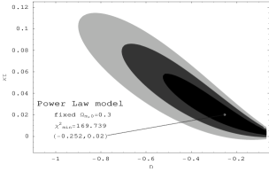
Figure 4: The $68.3\%$,$95.4\%$ and $99.7\%$ confidence contours of parameters $n$ and $\kappa\tau$ using the Gold SNeIa dataset and marginalizing over the model-independent parameter $\mu_{0}$ with a prior $\Omega_{m,0}=0.3$ in PL model.

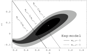
Figure 5: The $68.3\%$,$95.4\%$ and $99.7\%$ confidence contours of parameters $n$ and $\kappa\tau$ using the Gold SNeIa dataset and marginalizing over the model-independent parameter $\mu_{0}$ with a prior $\Omega_{m,0}=0.3$ in exp model. $w_{k,0}$ and $w_{t,0}$ are equation-of-state parameters of $\rho_{k}$ and $g(\rho_{m})$ at present time, respectively.

6 Discussion and conclusion

In above sections, we have investigated the viscous Cardassian cosmology for the expanding universe, assuming that there is a bulk viscosity in the cosmic fluid. We consider two solvable cases: (i) $\zeta=\sqrt{3}\kappa^{-1}\tau H$; (ii) $\zeta=\tau\left(g(\rho)\right)^{\alpha+\frac{3}{2}}$. In case (i), there exist exact solutions of $a$ as a function of $\Omega_{m,0}$ for PL, MP and exp models. Contrary to the naive PL model, in viscous PL model, the effective equation-of-state parameter $w_{k}$ is no longer a constant and it is dependent on time that can cross the cosmological constant divide $w_{\Lambda}=-1$ from $w_{k}>-1$ to $w_{k}<-1$. Other models possess with similar characteristics. For MP and exp models, $w_{k}$ evolves more near $-1$ than the case without viscosity. Moreover, the dynamical analysis indicates that there exists a singular curve in the phase diagram of viscous Cardassian .

On the other hand, the bulk viscosity can effect the collapse process of a bound system in the universe. We consider the virialization of a spherical collapse model using the spherical collapse formalism in PL Cardassian. The numerical result indicates that the parameter $\xi=\frac{R_{vir}}{R_{ta}}$ is always larger than $\frac{1}{2}$ and get larger and larger with the evolution of the universe. Furthermore, $\xi$ becomes larger when $\tau$ is increasing that means the bulk viscosity retards the progress of collapse system. Obviously, the bulk viscosity should be small to insure that the viscous cosmology theory isn’t in contradiction with the galaxy formation theory.

Using maximum likelihood technique, we constrain the parameters of viscous Cardassian models from the supernova data. If we assume prior that $\Omega_{m,0}=0.3$ as indicated by the observation about mass function of galaxies, the best fits of $\kappa\tau$ are $0.02$, $0.06$ and $0.07$ for PL, MP and exp models, respectively. In the following works, we plan to use other cosmological and astrophysical observations such as CMB, BAO and LSS to further constrain the viscous Cardassian parameters and the bulk viscosity coefficient.

References

- [1] S. Perlmutter et.al., Astrophys. J. 517 (1998) 565; A. G. Riess et.al., Astron. J. 116 (1998) 109.
- [2] P. de Bernardis et.al.,Nature. 404 (2000) 995; S. Hanany et.al., Astrophys. J. 545 (2000) L5; D. N. Spergel et.al.,Astrophys. J. Suppl. 170 (2007) 377.
- [3] M. Tegmark et.al., Astrophys. J. Suppl. 148 (2003) 175.
- [4] P. J. Steinhardt, L. Wang, I. Zlater, Phys. Rev. D59 (1999) 123504; X. Z. Li, J. G. Hao, D. J. Liu, Class. Quantum Grav. 19 (2002) 6049; D. J. Liu and X. Z. Li,Phys. Lett. B611 (2005) 8.
- [5] R. R. Caldwell, Phys. Lett. B545 (2002) 23; J. G. Hao and X. Z. Li, Phys. Rev. D67 (2003) 107303; J. G. Hao and X. Z. Li, Phys. Rev. D68 (2003) 043501;
- [6] K. Freese and M. Lewis, Phys. Lett. B540, (2002) 1.
- [7] K. Freese, Nucl. Phys. Proc. Suppl. 124 (2003) 50
- [8] P. Gondolo, K. Freese, Phys.Rev. D68, (2003) 063509.
- [9] S. Sen, A. A. Sen, Astron. J. 588 (2003) 1; W. J. Frith, Mon. Not. Roy. Astron. Soc. 348 (2004) 916; Z. H. Zhu, M. K. Fujimoto, Astron. J. 602 (2004) 12; C. Savage, N. Sugiyama, K. Freese, JCAP 0510 (2005) 007; T. Koivisto, H. Kurki-Suonio, F. Ravndal, Phys. Rev. D71 (2005) 064027; Z. L. Yi, T. J. Zhang, Phys. Rev. D75 (2007) 083515; F. Y. Wang, Z. G. Dai, JCAP 0708 (2007) 020.
- [10] D. J. Liu, C. B. Sun and X. Z. Li,Phys. Lett. B634 (2006) 442.
- [11] S. A. Balbus, Astrophys. J. 616 (2004) 857; B. F. Collins, H. E. Schlichting, R. Sari, Astron. J. 133 (2007) 2389.
- [12] S. Pratt,Phys. Rev. C77 (2008) 024910.
- [13] C. Eckart, Phys. Rev. 58 (1940) 919.
- [14] L. D. Landau and E. M. Lifshitz,Fluid Mechanics (Butterworth Heinemann, 1987).
- [15] W. Israel, Ann. Phys. 100 (1976) 310;
- [16] T. Harko, M. K. Mak, Class. Quant. Grav. 20 (2003) 407; M. Cataldo, N. Cruz, S. Lepe, Phys. Lett. B619 (2005) 5; X. H. Zhai, Y. D. Xu, X. Z. Li, Int. J. Mod. Phys. D15 (2006) 1151; R. Colistete, Jr. J. C. Fabris, J. Tossa, W. Zimdahl, Phys. Rev. D76 (2007) 103516; V. Folomeev, V. Gurovich,Phys. Lett. B661 (2008) 75.
- [17] A. Belinsky, I. M. Khalatnikov, Sov. Phys. JETP. 45 (1977) 1
- [18] W. Zimdahl, D. Pavón, Phys. Rev. D61 (2000) 108301.
- [19] Ø. Grøn, Astrophys. Space Sci. 173 (1990) 191.
- [20] J. G. Hao and X. Z. Li, Phys. Rev. D70, (2004) 043529; X. Z. Li, Y. B. Zhao, C. B. Sun,Class. Quant. Grav. 22 (2005) 3759.
- [21] J. E. Gunn and J. R. I. Gott, Astrophys. J. 176,(1972) 1.
- [22] I. Maor and O. Lahav, JCAP. 0507, (2005) 003.
- [23] A. G. Riess et.al., Astrophys. J. 659, (2007) 98.