A Unified Theory of Time-Frequency Reassignment

Abstract

Time-frequency representations such as the spectrogram are commonly used to analyze signals having a time-varying distribution of spectral energy, but the spectrogram is constrained by an unfortunate tradeoff between resolution in time and frequency. A method of achieving high-resolution spectral representations has been independently introduced by several parties. The technique has been variously named reassignment and remapping, but while the implementations have differed in details, they are all based on the same theoretical and mathematical foundation. In this work, we present a brief history of work on the method we will call the method of time-frequency reassignment, and present a unified mathematical description of the technique and its derivation. We will focus on the development of time-frequency reassignment in the context of the spectrogram, and conclude with a discussion of some current applications of the reassigned spectrogram.

,

1 Introduction

Many signals of interest have a distribution of energy that varies in time and frequency. For example, any sound signal having a beginning or an end has an energy distribution that varies in time, and most sounds exhibit considerable variation in both time and frequency over their duration. Time-frequency representations are commonly used to analyze or characterize such signals. They map the one-dimensional time-domain signal into a two-dimensional function of time and frequency. A time-frequency representation describes the variation of spectral energy distribution over time, much as a musical score describes the variation of musical pitch over time.

In audio signal analysis, the spectrogram is the most commonly-used time-frequency representation, probably because it is well-understood, and immune to so-called cross-terms that sometimes make other time-frequency representations difficult to interpret. But the windowing operation required in spectrogram computation introduces an unsavory tradeoff between time resolution and frequency resolution, so spectrograms provide a time-frequency representation that is blurred in time, in frequency, or in both dimensions.

Time-frequency reassignment is a technique for refocussing time-frequency data in a blurred representation like the spectrogram by mapping the data to time-frequency coordinates that are nearer to the true region of support of the analyzed signal. This method has been presented in other publications. In particular, the reader is referred to the excellent tutorial in [1] and to [2]. Time-frequency reassignment is gaining popularity, but it is still common to see new research conducted using the classical spectrogram that could benefit in efficiency or effectiveness from the enhancements afforded by reassignment.

In this paper, we will consider the application of time-frequency reassignment only to spectrogram data, though its effectiveness has also been demonstrated in the context of many other representations (see for example the extensive discussion of reassigned time-frequency representations and time-scale representations in [3]). For completeness, and because different formulations are popular in different research communities, we begin with a review of time-frequency analysis using the spectrogram in Section 2 before introducing the theory of time-frequency reassignment in Section 3. In Section 4 we discuss the notion of instantaneous frequency and its estimation using frequency reassignment. In Section 5, we introduce the condition called “separability”, which is crucial to obtain a meaningful time-frequency representation of a multicomponent signal.

Most common applications of the method of time-frequency reassignment are discrete (sampled) in time and frequency, so we next turn our attention to methods for efficiently estimating or computing reassigned time and frequency coordinates in the discrete case. Algorithms for implementing time-frequency reassignment have been presented in [1] and [2], but complete derivations of the techniques have not been published, to our knowledge, so in Section 6, we offer them as a useful starting point for future research in the computation of higher-order spectral derivatives.

We then consider some applications of the method of reassignment. In Section 7, we discuss improvements in spectrogram readability that can be achieved using reassigned data, with specific attention to methods of detecting and removing noisy or unreliable spectral data. In sound modeling applications, not only the spectral energy or magnitude is needed, but also the spectral phase. In Section 8, we discuss a high-fidelity additive sound model that is constructed from reassigned spectral data, and methods by which the short-time Fourier transform phase can be corrected to agree with the with the time-frequency estimates obtained by reassignment. Finally, in Section 9, we suggest some directions for future research using higher-order spectral derivatives.

2 The Spectrogram as a Time-Frequency Representation

One of the best-known time-frequency representations is the spectrogram, defined as the squared magnitude of the short-time Fourier transform

$$S(t,\omega)=|X(t,\omega)|^{2}.$$ (1)

The short-time Fourier transform is defined as a complex function of continuous time $t$ and radian frequency $\omega$ by

$$X(t,\omega) =\int x(\tau)h^{\ast}(t-\tau)e^{-j\omega\tau}d\tau$$ (2)

$$=\int x(\tau)h(t-\tau)e^{-j\omega\tau}d\tau$$ (3)

$$=M(t,\omega)e^{j\phi(t,\omega)}$$ (4)

where $h(t)$ is a finite-length, real-valued window function, (so $h(t)=h^{\ast}(t)$), $M(t,\omega)$ is the magnitude of the short-time Fourier transform, and $\phi(t,\omega)$ is its phase.

Often, it is more convenient to compute the time-varying spectrum by shifting the input signal, $x(t)$, instead of the window function. This modified transform, computed by

$$X_{t}(\omega) =\int x(\tau+t)h(-\tau)e^{-j\omega\tau}d\tau$$ (5)

$$=M_{t}(\omega)e^{j\phi_{t}(\omega)}$$ (6)

is simply the Fourier transform of the shifted and windowed input signal, $M_{t}(\omega)$ is the magnitude of the Fourier transform, and $\phi_{t}(\omega)$ is its phase.

Equations 3 and 5 differ in the range of $\tau$, the variable of integration, over which the integrand is non-zero. Since $h(t)$ is a finite-duration window function, the integrand in Equation 5 is always non-zero over the same range of $\tau$, for any $t$. Thus, the temporal reference of the transform “slides along” the signal, instead of remaining fixed at $t=0$, so we can call this transform the moving window transform [4], to distinguish it from the short-time Fourier transform.

The fixed range of integration in Equation 5 makes the moving window transform easy to implement directly in a digital system using a fast Fourier transform, but the two transforms are, in fact, equivalent, differing only in their temporal reference. By a change of variable, $t^{\prime}=\tau+t$, in Equation 5, we can show that

$$X_{t}(\omega) =\int x(\tau+t)h(-\tau)e^{-j\omega\tau}d\tau$$ (7)

$$=\int x(t^{\prime})h(t-t^{\prime})e^{j\omega(t-t^{\prime})}dt^{\prime}$$ (8)

$$=e^{j\omega t}\int x(t^{\prime})h(t-t^{\prime})e^{-j\omega t^{\prime}}dt^{\prime}$$ (9)

$$=e^{j\omega t}X(t,\omega)$$ (10)

$$=M(t,\omega)e^{j\left[\omega t+\phi(t,\omega)\right]}$$ (11)

so the moving window transform defined by Equation 5 is closely related to the short-time Fourier transform. The magnitudes of the two transforms are equal, and the phases differ only by a linear frequency term, that is,

$$M_{t}(\omega) =M(t,\omega)$$ (12)

$$\phi_{t}(\omega) =\omega t+\phi(t,\omega)$$ (13)

For a sinusoid having constant frequency, $\omega_{0}$, the phase of the short-time Fourier transform evaluated at that frequency, $\phi(t,\omega_{0})$, is constant for all time, and equal to the phase of the sinusoid at $t=0$, whereas $\phi_{t}(\omega_{0})$, the phase of the moving window transform evalutated at frequency $\omega_{0}$, rotates at exactly the frequency of the sinusoid.

Though the short-time phase spectrum is known to contain important temporal information about the signal, this information is difficult to interpret, so typically, only the short-time magnitude spectrum is considered in the construction of a time-frequency representation like the spectrogram. In the construction of additive sinusoidal sound models, the short-time phase spectrum is sometimes used to improve the frequency estimates in the time-frequency representation of quasi-harmonic sounds [5], but it is often omitted entirely, or used only in unmodified reconstruction, as in the Basic Sinusoidal Model, described by McAulay and Quatieri [6].

As a time-frequency representation, the spectrogram has relatively poor resolution. Time and frequency resolution are governed by the choice of analysis window, $h(t)$, and greater concentration in one domain is accompanied by greater smearing in the other. This smearing can be seen in Figures 1 and 2, which show spectrograms of a single pluck of an acoustic bass. The decaying part of the tone (after the pluck) is well-represented by nearly-harmonic sinusoidal components having a fundamental frequency of approximately 73.4 Hz. A very short-duration analysis window is needed in order to represent the temporal structure of the abrupt attack, but any window function short enough to provide the necessary temporal precision is much too wide in frequency to resolve the harmonic components of the tone (spaced at about 73.4 Hz). In Figure 1, the spectrogram has been computed using a 112.7 ms Kaiser window with a shaping parameter of 12. The harmonic components are resolved but the sharp attack is smeared by the duration of the analysis window. In Figure 2, the spectrogram has been computed using a much shorter Kaiser window (10 ms). The attack is less distorted but the harmonic structure is no longer discernible. The combination of poor resolution and poor precision often makes it necessary to use two or more spectrograms, like the two in Figures 1 and 2, to analyze an audio signal.

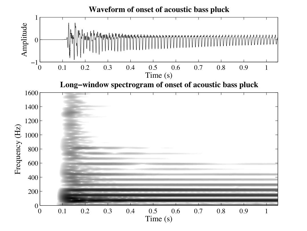
Figure 1: Spectrogram of an acoustic bass tone having a sharp pluck and a fundamental frequency of approximately 73.4 Hz. The spectrogram was computed using a 112.7 ms Kaiser window with a shaping parameter of 12. The harmonic components are resolved but the sharp attack is smeared by the duration of the analysis window.

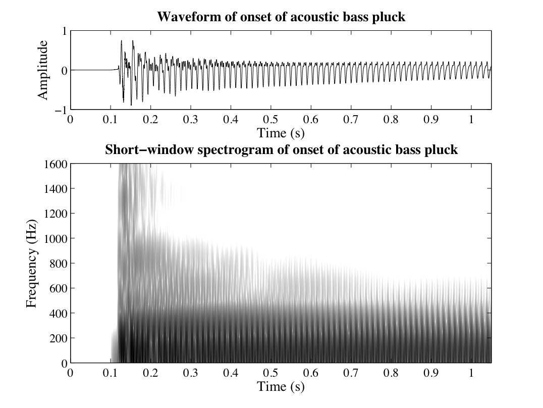
Figure 2: Spectrogram of an acoustic bass tone having a sharp pluck and a fundamental frequency of approximately 73.4 Hz. The spectrogram was computed using a 10 ms Kaiser window with a shaping parameter of 12. The attack is less distorted than in Figure 1 (though some smearing is still evident) but the harmonic structure is no longer discernible.

A time-frequency representation having improved resolution, relative to the spectrogram, is the Wigner-Ville distribution

$$W_{x}(t,\omega)=\int x(t+\tau/2)x^{\ast}(t-\tau/2)e^{-j\omega\tau}d\tau$$ (14)

which may be interpreted as a short-time Fourier transform  with a window function that is perfectly matched to the signal. The Wigner-Ville distribution is highly-concentrated in time and frequency, but it is also highly nonlinear and non-local. Consequently, this distribution is very sensitive to noise, and generates cross-components that often mask the components of interest, making it difficult to extract useful information concerning the distribution of energy in multi-component signals.

Cohen’s class of bilinear time-frequency representations  [7] is a class of “smoothed” Wigner-Ville distributions, defined

$$C_{x}(t,\omega)=\iint W_{x}(\tau,\nu)\Phi(\tau-t,\nu-\omega)d\tau d\nu$$ (15)

where $\Phi(t,\omega)$ is a smoothing kernel that can reduce sensitivity to noise and suppresses cross-components, at the expense of smearing the distribution in time and frequency. This smearing causes the distribution to be non-zero in regions where the true Wigner-Ville distribution shows no energy. $C_{x}(t,\omega)$ can be considered an average over a domain centered at the point $t,\omega$ of the values of the Wigner-Ville distribtuion at neighboring points $t-\tau,\omega-\Omega$ weighted by the value of the smoothing kernel $\Phi(\tau,\Omega)$.

The spectrogram in Equation 1 is a member of Cohen’s class. It is a smoothed Wigner-Ville distribution with the smoothing kernel equal to the Wigner-Ville distribution of the window function $h(t)$, that is,

$$\Phi(t,\omega)=W_{h}(t,\omega).$$ (16)

The method of reassignment smoothes the Wigner-Ville distribution, but then refocuses the distribution back to the true regions of support of the signal components. The method has been shown to reduce time and frequency smearing of any member of Cohen’s class [3], but we will focus here on its application to the spectrogram, and by extension, to short-time Fourier analysis of time-varying audio signals. In the case of the reassigned spectrogram, the short-time phase spectrum, $\phi(t,\omega)$, is used to correct the nominal time and frequency coordinates of the spectral data, and map it back nearer to the true regions of support of the analyzed signal.

3 The Method of Reassignment

Pioneering work on the method of reassignment was first published by Kodera, Gendrin, and de Villedary under the name of Modified Moving Window Method [4]. Their technique enhances the resolution in time and frequency of the classical Moving Window Method, the time-frequency representation constructed from the squared magnitude of the moving window transform defined in Equation 5, by assigning to each data point a new time-frequency coordinate that better-reflects the distribution of energy in the analyzed signal.

In the classical moving window method, a time-domain signal, $x(t)$ is decomposed into a set of coefficients, $\epsilon(t,\omega)$, based on a a set of elementary signals, $h_{\omega}(t)$, defined

$$h_{\omega}(t)=h(t)e^{j\omega t}$$ (17)

where $h(t)$ is a (real-valued) lowpass kernel function, like the window function in Equation 3. The coefficients in this decomposition are defined

$$\epsilon(t,\omega) =\int x(\tau)h(t-\tau)e^{-j\omega\left[\tau-t\right]}d\tau$$ (18)

$$=e^{j\omega t}\int x(\tau)h(t-\tau)e^{-j\omega\tau}d\tau$$ (19)

$$=e^{j\omega t}X(t,\omega)$$ (20)

$$=X_{t}(\omega)$$ (21)

In other words, the coefficients in the moving window method are computed from the moving window transform defined in Equation 5. In the moving window method, the time-frequency representation is constructed from the squared magnitude of the coefficients, and since the magnitude of these coefficients is identical to the magnitude of the short-time Fourier transform coefficients (see Equation 12), this time-frequency representation is exactly equivalent to the spectrogram.

$x(t)$ can be reconstructed from the moving window coefficients by

$$x(t) =\iint X_{\tau}(\omega)h^{\ast}_{\omega}(\tau-t)d\omega d\tau$$ (22)

$$=\iint X_{\tau}(\omega)h(\tau-t)e^{-j\omega\left[\tau-t\right]}d\omega d\tau$$ (23)

$$=\iint M_{\tau}(\omega)e^{j\phi_{\tau}(\omega)}h(\tau-t)e^{-j\omega\left[\tau-t\right]}d\omega d\tau$$ (24)

$$=\iint M_{\tau}(\omega)h(\tau-t)e^{j\left[\phi_{\tau}(\omega)-\omega\tau+\omega t\right]}d\omega d\tau$$ (25)

For signals having magnitude spectra, $M(t,\omega)$, whose time variation is slow relative to the phase variation, the maximum contribution to the reconstruction integral comes from the vicinity of the point $t,\omega$ satisfying the phase stationarity condition

$$\frac{\partial}{\partial\omega}\left[\phi_{\tau}(\omega)-\omega\tau+\omega t\right] =0$$ (26)

$$\frac{\partial}{\partial\tau}\left[\phi_{\tau}(\omega)-\omega\tau+\omega t\right] =0$$ (27)

or equivalently, around the point $\hat{t},\hat{\omega}$ defined by

$$\hat{t}(\tau,\omega) =\tau-\frac{\partial\phi_{\tau}(\omega)}{\partial\omega}=-\frac{\partial\phi(\tau,\omega)}{\partial\omega}$$ (28)

$$\hat{\omega}(\tau,\omega) =\frac{\partial\phi_{\tau}(\omega)}{\partial\tau}=\omega+\frac{\partial\phi(\tau,\omega)}{\partial\tau}.$$ (29)

This phenomenon has long been known in such fields as optics as the principle of stationary phase (see for example [8]). The principle of stationary phase states that for periodic or quasi-periodic signals, signals that are concentrated in frequency, the variation of the Fourier phase spectrum not attributable to periodic oscillation is slow with respect to time in the vicinity of the frequency of oscillation, and in surrounding regions the variation is relatively rapid. Analogously, for impulsive signals, that are concentrated in time, the variation of the phase spectrum is slow with respect to frequency near the time of the impulse, and in surrounding regions the variation is relatively rapid.

In sinusoidal reconstruction, positive and negative contributions to the synthesized waveform cancel, due to destructive interference, in frequency regions of rapid phase variation. Only regions of slow phase variation (stationary phase) will contribute significantly to the reconstruction, and the maximum contribution (center of gravity) occurs at the point where the phase is changing most slowly with respect to time and frequency.

The time-frequency coordinates computed by Equation 28 and Equation 29 are the local group delay, $\hat{t}_{g}(t,\omega)$, and local instantaneous frequency, $\hat{\omega}_{i}(t,\omega)$, and are computed from the phase of the short-time Fourier transform, which is normally ignored when constructing the spectrogram, though it is known to contain significant information about the signal. These quantities are “local” in the sense that they are represent a windowed and filtered signal that is localized in time and frequency, and are not global properties of the signal under analysis.

The modified moving window method changes (reassigns) the point of attribution of $\epsilon(t,\omega)$ to this point of maximum contribution $\hat{t}(t,\omega),\hat{\omega}(t,\omega)$, rather than to the point $t,\omega$ at which it is computed. This point is sometimes called the “center of gravity” of the distribution, by way of analogy to a mass distribution (in fact, Kodera et al. demonstrated that the coordinates $\hat{t}(t,\omega),\hat{\omega}(t,\omega)$ represent the center of gravity of Rihaczek’s complex energy distribution [9] for a real signal filtered by the short-time Fourier transform). This analogy is a useful reminder that the attribution of spectral energy to the center of gravity of its distribution only makes sense when there is energy to attribute, so the method of reassignment has no meaning at points where the spectrogram is zero-valued.

4 Local Estimation of Instantaneous Frequency

The group delay, defined in Equation 28, is often interpreted as the time delay, or average time, associated with a particular frequency, and its adoption as the reassigned temporal coordinate is consistent with that interpretation. In fact, it can easily be shown that the group delay (or equivalently, the time reassignment operation) exactly predicts the time of an impulse that lies in the region of support of the analysis window $h(t)$.

The notion of instantaneous frequency also has a long history in the signal processing literature, but it is normally computed from the signal phase, rather than the spectral phase. Specifically, when a signal is expressed in analytic form,

$$x(t)=A(t)e^{j\theta(t)}$$ (30)

where $A(t)$ is the (real) amplitude envelope and $\theta(t)$ is the (real) phase function, then the instantaneous frequency is defined as the derivative with respect to frequency of the signal phase, $\theta(t)$, that is

$$\omega_{i}(t)=\frac{d\theta(t)}{dt}$$ (31)

While it is clearly possible to obtain a single-component analytic representation of any signal (or, indeed, an infinite number of such representations), such a representation is not intuitively satisfying for most audio signals. Pitched sounds, such as musical instrument tones, are characterized by quasi-harmonic spectra, and a representation as a sum of components representing the various harmonic partials is more revealing and intuitive. Vocal sounds are often analyzed as the response of a resonant system (the vocal tract) to some excitation signal, and a multicomponent representation that identifies the formants of the resonant system is more informative.

A crucial insight in the development of the method of frequency reassignment follows from the interpretation of the short-time Fourier transform as a demodulated bank of linear time-invariant bandpass filters, wherein each filter, $h_{\omega}(t)$, has an impulse response determined by

$$h_{\omega}(t)=h(t)e^{j\omega t}$$ (32)

Since the window function, $h(t)$ is the impulse response of a finite impulse response lowpass filter, the modulated window function is the impulse response of a finite impulse response bandpass filter with passband centered at frequency $\omega$. Since $h(t)$ is real, $h_{\omega}(t)$ is complex and, therefore, describes a filter having an assymmetric frequency response. An analogous bandpass filter having a real impulse response would pass frequencies around $\pm\omega$, but $h_{\omega}(t)$ passes only frequencies around $\omega$.

In the filterbank interpretation of the short-time Fourier transform, $X(t,\omega)$ describes the output of a bank of such filters excited by the input signal, $x(t)$. That is,

$$X(t,\omega) =\int x(\tau)h(t-\tau)e^{-j\omega\tau}d\tau$$ (33)

$$=\int x(\tau)h(t-\tau)e^{j\omega\left[t-\tau\right]}e^{-j\omega t}d\tau$$ (34)

$$=e^{-j\omega t}\int x(\tau)h_{\omega}(t-\tau)d\tau$$ (35)

$$=e^{-j\omega t}\left[x(t)\ast h_{\omega}(t)\right]$$ (36)

In this interpretation, $X(t,\omega_{0})$ describes the demodulated output of a single bandpass filter, centered at frequency $\omega_{0}$. The output of the filter is considered to be a single complex exponential having magnitude $M(t,\omega_{0})$ and a phase composed of a linear component, due to sinusoidal oscillation at frequency $\omega_{0}$, and another time-varying component, $\phi(t,\omega_{0})$, accounting for the deviation from pure sinusoidal oscillation at frequency $\omega_{0}$. $X(t,\omega_{0})$ is the output of the filter demodulated to remove the sinusoidal oscillation at frequency $\omega_{0}$, and the output of the moving window transform $X_{t}(\omega_{0})=X(t,\omega_{0})e^{j\omega_{0}t}$, is the raw output of the bandpass filter centered at frequency $\omega_{0}$.

Kodera et al. [4] showed that the local instantaneous frequency, computed from the derivative with respect to time of the spectral phase, $\phi(t,\omega)$, is equal to the instantaneous frequency of the bandpass filtered signal that is the output of the short-time Fourier transform at the coordinates $t,\omega$. For a signal

$$x(t)=A(t)e^{j\theta(t)}$$ (37)

having instantaneous frequency

$$\omega_{i}(t)=\frac{d\theta(t)}{dt},$$ (38)

$X(t,\omega_{0})e^{j\omega_{0}t}$ is the output of the bandpass filter $h_{\omega_{0}}(t)$, centered at frequency $\omega_{0}$, when the input is $x(t)$. If, at time $t$, the instantaneous frequency of the input, $\omega_{i}(t)$ is far from $\omega_{0}$, such that the instantaneous frequency of the input is outside the passband of the filter centered at $\omega_{0}$, then the output of the filter is essentially zero. If, on the other hand, $\omega(t)$, is within the passband of the filter (near $\omega_{0}$), then the signal passes through the filter unaltered except for a scale factor, equal to the passband gain, and a constant time delay, so its instantaneous frequency can be computed from the phase of the response of $h_{\omega_{0}}(t)$ or any filter that passes $x(t)$.

The filters that comprise the short-time Fourier transform introduce only a constant offset to the phase of any component that they pass, and the spectral phase obtained from the response of a single short-time Fourier transform filter differs only by a constant offset from the phase of a single component whose frequency lies in the passband of that filter. Therefore, the derivative with respect to time of the filtered signal, $X_{t}(\omega)$, is equal to the derivative with respect to time of the original signal, $x(t)$, and so the instantaneous frequency of that component can be computed from the phase of the short-time Fourier transform evaluated at $\omega$. That is,

$$\omega_{i}(t) =\frac{\partial}{\partial t}\arg\{x(t)\}$$ (39)

$$=\frac{\partial}{\partial t}\arg\{X_{t}(\omega)\}$$ (40)

$$=\frac{\partial}{\partial t}\arg\{e^{j\omega t}X(t,\omega)\}$$ (41)

$$=\omega+\frac{\partial\phi(t,\omega)}{\partial t}$$ (42)

$$=\hat{\omega}(t,\omega)$$ (43)

for any $\omega$ such that $h_{\omega}(t)$ is the impulse response of a filter that passes $x(t)$.

The short-time Fourier transform filters may also introduce a time delay (if, for example, the frequency of the signal under analysis is not exactly equal to the center frequency of the filter), but this delay is precisely the group delay. Therefore, the local instantaneous frequency computed from the derivative with respect to time of the spectral phase is equal to the instantaneous frequency of the signal at a time offset from the center of the analysis window by the group delay, computed from the derivative with respect to frequency of the spectral phase. The short-time Fourier transform coefficients evaluated at time $t$ and frequency $\omega$ are mapped from the geometric center of the analysis window ($t,\omega$) onto the region of support of the analyzed signal by the reassignment operations in Equation 28 and Equation 29.

The term local instantaneous frequency indicates that $\hat{\omega}(t,\omega)$ is the instantaneous frequency of the dominant component at a particular time and frequency. Nelson calls it the channelized instantaneous frequency [10, 11], to emphasize that it is the instantaneous frequency of a component passing through a single short-time Fourier transform channel. Flanagan also showed that instantaneous frequency could be computed for each short-time Fourier transform bin from partial derivatives of the phase spectrum [12], and his method has been widely used for obtaining estimates of fundamental frequency (see for example [13] and [14]).

Figure 3 demonstrates the effect of frequency reassignment for a fragment of voiced speech. The upper plot shows the conventional (dashed lines) and reassigned (crosses) magnitude spectra. The lower plot shows the mapping of nominal (Fourier transform bin) frequency to reassigned frequency for the same fragment of speech. Near the frequencies of strong harmonics, the mapping is flat, as all nearby transform data is reassigned to the frequency of the dominant harmonic component. This consensus, or clustering among reassigned frequency estimates in the vicinity of spectral peaks can be used as an indicator of the reliability of the time-frequency data [15]. If the reassigned frequencies for neighboring short-time Fourier transform channels are all very similar, then there is said to be a high degree of consensus and the quality of the frequency estimates is assumed to be good.

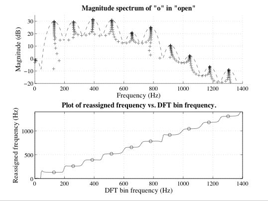
Figure 3: Demonstration of frequency reassignment in a single spectrum for a fragment of speech (the “o” in “open”), computed using a 33.6 ms Kaiser analysis window with a shaping parameter of 12. The upper plot shows the conventional (dashed lines) and reassigned (crosses) magnitude spectra. The lower plot shows the mapping of nominal (Fourier transform bin) frequency to reassigned frequency for the same fragment of speech. The flat portions of the lower curve represent regions in which the energy in many transform bins is reassigned to the same frequency. The circled points show the samples having locally minimal frequency reassignments.

The method of time-frequency reassignment has been used in a variety of applications for obtaining improved time and frequency estimates for time-varying spectral data [16, 17, 18]. Often, only the frequency reassignment operation is used to compute instantaneous frequency estimates [13, 15]. It should be noted that, for many choices of analysis window, the much simpler method of parabolic interpolation of the magnitude spectrum, proposed by Smith and Serra [19] gives very similar frequency estimates (and in some cases, even more precise estimates, according to [20]). We are, however, aware of no competing method for improving the accuracy of the time estimates in short-time spectral analysis.

5 Separability

The short-time Fourier transform can often be used to estimate the amplitudes and phases of the individual components in a multi-component signal, such as a quasi-harmonic musical instrument tone (see, for example, [5]). Moreover, the time and frequency reassignment operations described by Equation 28 and Equation 29 can be used to sharpen the representation by attributing the spectral energy reported by the short-time Fourier transform to the point that is the local center of gravity of the complex energy distribution [18].

For a signal consisting of a single component, described by Equation 37, the instantaneous frequency can be estimated from the partial derivatives of phase of any short-time Fourier transform channel that passes the component, as shown above. If the signal is to be decomposed into many components,

$$x(t)=\sum_{n}A_{n}(t)e^{j\theta_{n}(t)}$$ (44)

and the instantaneous frequency of each component is defined as the derivative of its phase with respect to time, that is,

$$\omega_{n}(t)=\frac{d\theta_{n}(t)}{dt},$$ (45)

then the instantaneous frequency of each individual component can be computed from the phase of the response of a filter that passes that component, provided that no more than one component lies in the passband of the filter.

This is the property, in the frequency domain, that Nelson called “separabilty” [10, 11] and we require this property of all the signals we analyze. If this property is not met, then we cannot achieve the desired multicomponent decomposition, because we can not estimate the parameters of individual components from the short-time Fourier transform and we must choose a different analysis window so that the separability criterion is satisfied.

If the components of a signal are separable in frequency with respect to a particular short-time spectral analysis window, then the output of each short-time Fourier transform filter is a filtered version of, at most, a single dominant (having significant energy) component, and so the derivative, with respect to time, of the phase of the $X(t,\omega_{0})$ is equal to the derivative with respect to time, of the phase of the dominant component at $\omega_{0}$. Therefore, if a component, $x_{n}(t)$, having instantaneous frequency $\omega_{n}(t)$ is the dominant component in the vicinity of $\omega_{0}$, then the instantaneous frequency of that component can be computed from the phase of the short-time Fourier transformevaluated at $\omega_{0}$. That is,

$$\omega_{n}(t) =\frac{\partial}{\partial t}\arg\{x_{n}(t)\}$$ (46)

$$=\frac{\partial}{\partial t}\arg\{X(t,\omega_{0})\}$$ (47)

Thus, the partial derivative with respect to time of the phase of the short-time Fourier transform can be used to compute the instantaneous frequencies of the individual components in a signal described by Equation 44, provided only that the components are separable in frequency by the chosen analysis window.

Just as we require that each bandpass filter in the short-time Fourier transform filterbank pass at most a single complex exponential component, we require that two temporal events be sufficiently separated in time that they do not lie in the same windowed segment of the input signal. This is the property of separability in the time domain, and is equivalent to requiring that the time between two events be greater than the length of the impulse response of the short-time Fourier transform filters, the span of non-zero samples in $h(t)$.

Separability in time and in frequency is required of components we wish to resolve in a reassigned time-frequency representation. If the components in a decomposition are separable in time and frequency in a certain time-frequency representation, then the components can be resolved by that time-frequency representation, and using the method of reassignment, can be characterized with much greater precision than is possible using classical methods.

For any signal, there are an infinite number of decompositions of the form given in Equation 44. The separability property must be considered in the context of the desired decomposition. Figure 4 shows a reassigned spectrogram of a speech signal computed using an analysis window that is long relative to the time between glottal pulses. The harmonics are clearly visible, and the formant frequencies can also be discerned, but the individual glottal pulses are smeared in this representation, because many pulses are covered by each analysis window (that is, the individual pulses are not separable, in time, by the chosen analysis window). Figure 5 shows a spectrogram of the same speech signal computed using an analysis window that is much shorter than the time between glottal pulses. In this representation, the individual pulses are clearly visible, because no window spans more than one pulse, but the harmonic frequencies are not visible, because the main lobe of the analysis window spectrum is much wider than the spacing between the harmonics (that is, the harmonics are not separable, in frequency, by the chosen analysis window).

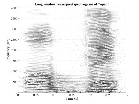
Figure 4: Long-window reassigned spectrogram of the word “open”, computed using a 54.4 ms Kaiser window with a shaping parameter of 9, emphasizing harmonics.

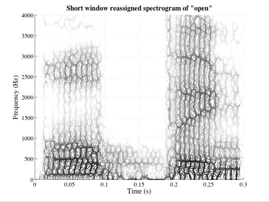
Figure 5: Short-window reassigned spectrogram of the word “open”, computed using a 13.6 ms Kaiser window with a shaping parameter of 9, emphasizing formants and glottal pulses.

6 Efficient Computation of Reassigned Times and Frequencies

In digital signal processing, it is most common to sample the time and frequency domains. The discrete Fourier transform is used to compute samples $X(k)$ of the Fourier transform from samples $x(n)$ of a time domain signal,

$$X(k)=\sum_{m=0}^{N-1}x(m)e^{\frac{-j2\pi km}{N}}$$ (48)

where $x(n)$ is the time domain signal sampled at $t_{n}=nT$ for sampling period $T$, $X(k)$ is the discrete Fourier transform coefficients, equal (for adequately-sampled bandlimited signals) to samples of the Fourier transform at (radian) frequencies $\omega_{k}=2\pi k/N$. For highly-composite $N$, such as powers of two, the discrete Fourier transform can be computed very efficiently using a fast Fourier transform algorithm.

The discrete short-time Fourier transform can be computed

$$X(n,k) =\sum_{m=n-N+1}^{n}x(m)h(n-m)e^{\frac{-j2\pi km}{N}}$$ (49)

$$=e^{\frac{j2\pi kn}{N}}\sum_{m=0}^{N-1}x(m+n)h(-m)e^{\frac{-j2\pi km}{N}}$$ (50)

$$=e^{\frac{j2\pi kn}{N}}X_{n}(k)$$ (51)

where $h(n)$ is samples of a real-valued, finite-length window function that is non-zero only on the range $n=0\ldots N-1$, and is analogous to the analysis window $h(t)$ in Equation 3. $X_{n}(k)$ is the discrete Fourier transform of a shifted and windowed input signal, the discrete time moving window transform defined in Equation 5. For a signal sampled with sampling period $T$ seconds, the $N$-point discrete short-time Fourier transform computes samples of the short-time Fourier transform at times $t_{n}=nT$ and (radian) frequencies $\omega_{k}=2\pi k/N$.

The reassignment operations proposed by Kodera et al. cannot be applied to the discrete short-time Fourier transform data, because partial derivatives cannot be computed directly on data that is discrete in time and frequency. It has been suggested that this difficulty has been the primary barrier to wider use of the method of reassignment [21].

6.1 Approximation of the Partial Derivatives of Phase

It is possible to approximate the partial derivatives using finite differences. For example, the phase spectrum can be evaluated at two nearby times, and the partial derivative with respect to time be approximated as the difference between the two values divided by the time difference, as in:

$$\frac{\partial\phi(t,\omega)}{\partial t} \approx\frac{1}{\Delta t}\left[\phi(t+\frac{\Delta t}{2},\omega)-\phi(t-\frac{\Delta t}{2},\omega)\right]$$ (52)

$$\frac{\partial\phi(t,\omega)}{\partial\omega} \approx\frac{1}{\Delta\omega}\left[\phi(t,\omega+\frac{\Delta\omega}{2})-\phi(t,\omega-\frac{\Delta\omega}{2})\right]$$ (53)

For sufficiently small values of $\Delta t$ and $\Delta\omega$, this finite-difference method yields good approximations to the partial derivatives of phase, because in regions of the spectrum in which the evolution of the phase is dominated by rotation due to sinusoidal oscillation of a single, nearby component, the phase is a linear function.

But the phase of the Fourier transform is the argument of a complex quantity, and can only be computed modulo $2\pi$. This phase wrapping effect, that equates all phases differing by a multiple of $2\pi$, has no practical impact on the individual phase values, but is of some consequence when two phases are combined as in the finite difference derivative approximation, because the difference between two phase values may not be preserved by the wrapping process.

Fortunately, $\Delta t$ and $\Delta\omega$, can be chosen to be small enough that, for a properly-sampled signal, the phase difference can be easily “unwrapped”. The absolute value of the difference in phase between consecutive samples, in time or in frequency, of the short-time Fourier transform cannot exceed $\pi$ in any region of the spectrum dominated by a significant oscillating component. Any phase difference that exceeds $\pi$, in the absolute sense, has been corrupted by phase wrapping, and can be corrected by simply adding or subtracting $2\pi$ to obtain an absolute value that is less than $\pi$. Thus, if $\Delta t$ and $\Delta\omega$ are chosen to be one sample, then the finite difference method can be used to accurately-estimate the reassigned times and frequencies in regions of the spectrum in which the evolution of the phase is dominated by rotation due to sinusoidal oscillation of a nearby component.

Charpentier [22] used a finite difference approximation to Flanagan’s instantaneous frequency equation [12] and showed that the approximation could be computed using only a single Fourier transform for the case of the Hann analysis window.

Unaware of the work of Kodera et al., Nelson arrived at a similar method for computing reassigned time-frequency coordinates for short-time spectral data from partial derivatives of the short-time phase spectrum [10, 11]. Instead of directly computing the first differences of phase, Nelson first computes two so-called cross spectral surfaces,

$$C(t,\omega) =X(t+\frac{\Delta t}{2},\omega)X^{\ast}(t-\frac{\Delta t}{2},\omega)$$ (54)

$$L(t,\omega) =X(t,\omega+\frac{\Delta\omega}{2})X^{\ast}(t,\omega-\frac{\Delta\omega}{2})$$ (55)

The partial derivatives are then approximated by the phase of these cross spectra.

$$\frac{\partial\phi(t,\omega)}{\partial t} \approx\frac{1}{\Delta t}\arg(C(t,\omega))$$ (56)

$$\frac{\partial\phi(t,\omega)}{\partial\omega} \approx\frac{1}{\Delta\omega}\arg(L(t,\omega))$$ (57)

It is easily shown that approximation of the derivatives by means of a cross spectral surface is equivalent to computing the finite differences directly, only the differences are unwrapped automatically when the argument is computed, for example:

$$\frac{1}{\Delta t}\arg(C(t,\omega)) =\frac{1}{\Delta t}\arg\left(X(t+\frac{\Delta t}{2},\omega)X^{\ast}(t-\frac{\Delta t}{2},\omega)\right)$$ (58)

$$=\frac{1}{\Delta t}\arg\left(M(t+\frac{\Delta t}{2},\omega)e^{j\phi(t+\frac{\Delta t}{2},\omega)}M(t-\frac{\Delta t}{2},\omega)e^{-j\phi(t-\frac{\Delta t}{2},\omega)}\right)$$ (59)

$$=\frac{1}{\Delta t}\arg\left(M(t+\frac{\Delta t}{2},\omega)M(t-\frac{\Delta t}{2},\omega)e^{j\left[\phi(t+\frac{\Delta t}{2},\omega)-\phi(t-\frac{\Delta t}{2},\omega)\right]}\right)$$ (60)

$$=\frac{1}{\Delta t}\left[\phi(t+\frac{\Delta t}{2},\omega)-\phi(t-\frac{\Delta t}{2},\omega)\right]$$ (61)

While these linear differences only approximate the partial derivatives of the phase with respect to time and frequency, they give very good approximations in regions of the spectrum dominated by a single, significant concentration of energy, such as an impulse or a sinusoid, because in these regions the evolution of the phase spectrum is linear in time and in frequency. In regions of the spectrum having no significant concentration of energy, the finite difference approximation may not be a good one, but it makes little sense to compute reassigned time and frequency coordinates when there is no energy to reassign.

6.2 Evaluation of the Partial Derivatives of Phase Using Transforms

Auger and Flandrin [3] showed how the method of reassignment, proposed in the context of the spectrogram by Kodera et al., could be extended to any member of Cohen’s class of time-frequency representations by generalizing the reassignment operations in Equation 28 and Equation 29 to

$$\hat{t}(t,\omega) =t-\frac{\iint\tau\cdot W_{x}(t-\tau,\omega-\nu)\cdot\Phi(\tau,\nu)d\tau d\nu}{\iint W_{x}(t-\tau,\omega-\nu)\cdot\Phi(\tau,\nu)d\tau d\nu}$$ (62)

$$\hat{\omega}(t,\omega) =\omega-\frac{\iint\nu\cdot W_{x}(t-\tau,\omega-\nu)\cdot\Phi(\tau,\nu)d\tau d\nu}{\iint W_{x}(t-\tau,\omega-\nu)\cdot\Phi(\tau,\nu)d\tau d\nu}$$ (63)

where $W_{x}(t,\omega)$ is the Wigner-Ville distribution of $x(t)$, and $\Phi(t,\omega)$ is the kernel function that defines the distribution. They further described an efficient method for computing the times and frequencies for the reassigned spectrogram efficiently and accurately without explicitly computing the partial derivatives of phase.

In the case of the spectrogram, $S_{x}(t,\omega)=|X(t,\omega)|^{2}$, the reassignment operations in Equation 28 and Equation 29 can be computed by

$$\hat{t}(t,\omega) =t-\Re\Bigg{\{}\frac{X_{\mathcal{T}h}(t,\omega)\cdot X^{\ast}(t,\omega)}{|X(t,\omega)|^{2}}\Bigg{\}}$$ (64)

$$\hat{\omega}(t,\omega) =\omega+\Im\Bigg{\{}\frac{X_{\mathcal{D}h}(t,\omega)\cdot X^{\ast}(t,\omega)}{|X(t,\omega)|^{2}}\Bigg{\}}$$ (65)

where $X(t,\omega)$ is the short-time Fourier transform computed using an analysis window $h(t)$, $X_{\mathcal{T}h}(t,\omega)$ is the short-time Fourier transform computed using a time-weighted anlaysis window $h_{\mathcal{T}}(t)=t\cdot h(t)$ and $X_{\mathcal{D}h}(t,\omega)$ is the short-time Fourier transform computed using a time-derivative analysis window $h_{\mathcal{D}}(t)=\frac{d}{dt}h(t)$.

In this method, using the auxiliary window functions $h_{\mathcal{T}}(t)$ and $h_{\mathcal{D}}(t)$, the reassignment operations can be computed at any time-frequency coordinate $t,\omega$ from an algebraic combination of the values of three Fourier transforms evaluated at $t,\omega$, without directly evaluating or approximating the partial derivatives of phase. A method of computing instantaneous frequency equivalent to Equation 65 was independently discovered by Abe [23], and is sometimes used in fundamental frequency estimation (see for example [13]). Since the these algorithms operate only on spectral data evaluated at a single time and frequency, and do not explicitly compute any derivatives, they can easily be implemented in digital systems using discrete times and frequencies.

The time-weighted window function, $h_{\mathcal{T}}(t)$, is trivially computed by pointwise multiplication of the original window function, $h(t)$, by a time ramp. If the derivative of the window function is unknown, then $h_{\mathcal{D}}(t)$ can also be computed numerically. The derivative theorem for Fourier transforms, which states that if $X(\omega)$ is the Fourier transform of $x(t)$, then the Fourier transform of $\frac{d}{dt}x(t)$ is $j\omega X(\omega)$. That is,

$$x(t)\leftrightarrow X(\omega)$$ (66)

implies

$$\frac{d}{dt}x(t)\leftrightarrow j\omega X(\omega)$$ (67)

We can therefore construct the time-derivative window used in the evaluation of the frequency reassignment operator by computing the Fourier transform of $h(t)$, multiplying by $j\omega$, and inverting the Fourier transform. That is,

$$\frac{d}{dt}h(t) =\mathrm{FFT}^{-1}\{j\omega H(\omega)\}$$ (68)

$$=-\Im\Big{\{}\mathrm{FFT}^{-1}\{\omega H(\omega)\}\Big{\}}$$ (69)

and so, in discrete time,

$$h_{\mathcal{D}}(n)=-\Im\Big{\{}\mathrm{FFT}^{-1}\big{\{}\frac{2\pi k}{N}H(k)\big{\}}\Big{\}}$$ (70)

The auxiliary short-time analysis windows employed in the computation of Auger and Flandrin’s reassignment operations are shown in Figure 6 for the case of $h(n)$ being 501 samples at 44.1 kHz of a Kaiser window with shaping parameter equal to 12.

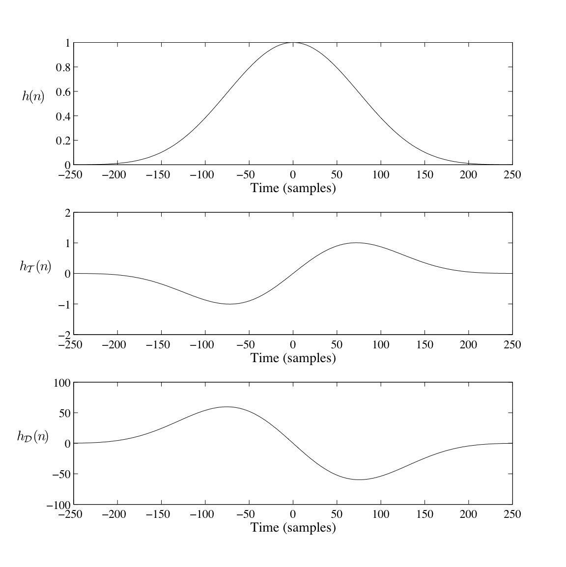
Figure 6: Representative analysis windows employed in the three short-time transforms used to compute reassigned times and frequencies. Waveform (a) is the original window function, $h(n)$ (a Kaiser window with shaping parameter 12.0, in this case), waveform (b) is the time-weighted window function, $h_{\mathcal{T}}(n)$, and waveform (c) is the frequency-weighted window function, $h_{\mathcal{D}}(n)$. In each case, the plots were made from 501 samples of the corresponding window function at 44.1 kHz.

Using Equation 64 and Equation 65, the value of the reassignment operations at $t,\omega$ can be computed from the values of the three short-time Fourier transforms at $t,\omega$, without direct evaluation of any partial derivatives. So if the values of the transforms at discrete time and frequency coordinates, $t_{n},\omega_{k}$, are known, then the values of the reassignment operations can be computed for those discrete times and frequencies without resorting to discrete approximations to the partial derivatives in Equation 28 and Equation 29. Since the discrete short-time Fourier transform computes the values of the short-time Fourier transform at discrete times and frequencies, values of the reassignment operations, $\hat{\omega}(t_{n},\omega_{k})$ and $\hat{t}(t_{n},\omega_{k})$ can be computed from three discrete short-time Fourier transforms. This gives an efficient method of computing the reassigned discrete short-time Fourier transform provided only that the $|X(t,\omega)|^{2}$ is non-zero. This is not much of a restriction, since the reassignment operation itself implies that there is some energy to reassign, and has no meaning when the distribution is zero-valued.

In the two sections that follow, we derive the reassignment operations proposed by Auger and Flandrin. The implementation of the reassignment operations has been described elsewhere [1, 2], and partial derivations have been presented (see, for example [3] and [21]), but we are not aware of a complete, published derivation. We include the derivations here for completeness, and because we have found them to be a useful starting point for deriving methods of computing other spectral derivatives.

The procedure in each derivation is the same. First, we show that the partial derivative of the spectral phase can be expressed in terms of the short-time Fourier transform and its partial derivative. Then, we show that the partial derivative of the short-time Fourier transform can be computed from the transform itself and a second transform computed using a different window function. Finally, we combine the results to obtain an expression for the reassigned coordinate that does not include any explicit partial derivatives.

Readers not interested in the mathematical derivation of the reassignment operations can skip ahead to Section 7.

6.2.1 Derivation of Efficient Spectrogram Time Reassignment Operator

In this section, we present the mathematical derivation of the efficient time reassignment operator discovered by Auger and Flandrin. In Section 6.2.2 we will present the derivation of the frequency reassignment operator. We begin by restating the time reassignment operation identified by Kodera et. al., and presented here in Equation 28

$$\hat{t}(t,\omega)=-\frac{\partial\phi(t,\omega)}{\partial\omega}.$$

To arrive at an expression for the partial derivative of spectral phase with respect to frequency, we first take the partial derivative of $X(t,\omega)$ with respect to frequency. Applying the product rule of differential calculus to Equation 4,

$$\frac{\partial}{\partial\omega}X(t,\omega) =\frac{\partial}{\partial\omega}\left[M(t,\omega)e^{j\phi(t,\omega)}\right]$$ (71)

$$=\frac{\partial M(t,\omega)}{\partial\omega}\cdot e^{j\phi(t,\omega)}+M(t,\omega)\cdot j\frac{\partial\phi(t,\omega)}{\partial\omega}e^{j\phi(t,\omega)}$$ (72)

$$=\frac{\partial M(t,\omega)}{\partial\omega}\cdot e^{j\phi(t,\omega)}+j\frac{\partial\phi(t,\omega)}{\partial\omega}X(t,\omega)$$ (73)

In order to isolate the partial derivative of phase, we can multiply by $jX^{\ast}(t,\omega)/|X(t,\omega)|^{2}$ (this operation is only valid when $|X(t,\omega)|^{2}$ is non-zero, but as noted earlier, the reassignment operation itself has no meaning when the distribution is zero-valued) and simplify to obtain

$$\left[\frac{\partial}{\partial\omega}X(t,\omega)\right]\cdot\frac{jX^{\ast}(t,\omega)}{|X(t,\omega)|^{2}} =\left[\frac{\partial M(t,\omega)}{\partial\omega}\cdot e^{j\phi(t,\omega)}+j\frac{\partial\phi(t,\omega)}{\partial\omega}\cdot X(t,\omega)\right]\cdot\frac{jX^{\ast}(t,\omega)}{|X(t,\omega)|^{2}}$$ (74)

$$=\frac{\partial M(t,\omega)}{\partial\omega}\cdot e^{j\phi(t,\omega)}\cdot\frac{jX^{\ast}(t,\omega)}{|X(t,\omega)|^{2}}-\frac{\partial\phi(t,\omega)}{\partial\omega}\cdot\frac{|X(t,\omega)|^{2}}{|X(t,\omega)|^{2}}$$ (75)

$$=\frac{\partial M(t,\omega)}{\partial\omega}\cdot\frac{jM(t,\omega)}{|X(t,\omega)|^{2}}-\frac{\partial\phi(t,\omega)}{\partial\omega}$$ (76)

$$=-\frac{\partial\phi(t,\omega)}{\partial\omega}+j\cdot\left[\frac{M(t,\omega)}{|X(t,\omega)|^{2}}\right]\cdot\frac{\partial M(t,\omega)}{\partial\omega}$$ (77)

Since $M(t,\omega)$ is real-valued, the real part of this expression is precisely the negative partial derivative with respect to frequency of the phase of the short-time Fourier transform. Thus, we conclude that the partial derivative of spectral phase with respect to frequency, and hence, the reassigned time, $\hat{t}$, can be computed by

$$\hat{t}(t,\omega)=-\frac{\partial\phi(t,\omega)}{\partial\omega}=\Re\Bigg{\{}\frac{\partial X(t,\omega)}{\partial\omega}\cdot\frac{jX^{\ast}(t,\omega)}{|X(t,\omega)|^{2}}\Bigg{\}}$$ (78)

Equation 78 expresses the partial derivative of the short-time Fourier transform phase with respect to frequency in terms of the transform itself and its partial derivative with respect to frequency.

Next, we will show that the partial derivative of the short-time Fourier transform with respect to frequency can be computed without explicitly computing or approximating any derivatives. Taking the partial derivative of the short-time Fourier transform given by Equation 3,

$$\frac{\partial}{\partial\omega}X(t,\omega) =\frac{\partial}{\partial\omega}\int x(\tau)h(t-\tau)e^{-j\omega\tau}d\tau$$ (79)

$$=\int x(\tau)h(t-\tau)\left[\frac{\partial}{\partial\omega}e^{-j\omega\tau}\right]d\tau$$ (80)

$$=\int x(\tau)h(t-\tau)\left[-j\tau e^{-j\omega\tau}\right]d\tau$$ (81)

$$=-j\int x(\tau)\cdot\tau\cdot h(t-\tau)e^{-j\omega\tau}d\tau$$ (82)

$$=-jtX(t,\omega)+jtX(t,\omega)-j\int x(\tau)\cdot\tau\cdot h(t-\tau)e^{-j\omega\tau}d\tau$$ (83)

$$=-jtX(t,\omega)+j\int x(\tau)\cdot(t-\tau)\cdot h(t-\tau)e^{-j\omega\tau}d\tau$$ (84)

$$=-jtX(t,\omega)+j\int x(\tau)h_{\mathcal{T}}(t-\tau)e^{-j\omega\tau}d\tau$$ (85)

$$=-jtX(t,\omega)+jX_{\mathcal{T}h}(t,\omega)$$ (86)

where $h_{\mathcal{T}}(t)=t\cdot h(t)$ is the time-weighted anlaysis window described in Section 6 and shown in Figure 6, and $X_{\mathcal{T}h}(t,\omega)$ is the short-time Fourier transform computed using this time-weighted analysis window. Multiplying, as before (and with the same caveat concerning zero-valued distributions), by $jX^{\ast}(t,\omega)/|X(t,\omega)|^{2}$, we obtain

$$\left[\frac{\partial}{\partial\omega}X(t,\omega)\right]\cdot\frac{jX^{\ast}(t,\omega)}{|X(t,\omega)|^{2}} =\left[-jtX(t,\omega)+jX_{\mathcal{T}h}(t,\omega)\right]\cdot\frac{jX^{\ast}(t,\omega)}{|X(t,\omega)|^{2}}$$ (87)

$$=t\cdot\frac{|X(t,\omega)|^{2}}{|X(t,\omega)|^{2}}+\frac{jX_{\mathcal{T}h}(t,\omega)\cdot jX^{\ast}(t,\omega)}{|X(t,\omega)|^{2}}$$ (88)

$$=t-\frac{X_{\mathcal{T}h}(t,\omega)\cdot X^{\ast}(t,\omega)}{|X(t,\omega)|^{2}}$$ (89)

Substituting this expression into Equation 78, we obtain

$$\hat{t}(t,\omega)=-\frac{\partial\phi(t,\omega)}{\partial\omega}=t-\Re\Bigg{\{}\frac{X_{\mathcal{T}h}(t,\omega)\cdot X^{\ast}(t,\omega)}{|X(t,\omega)|^{2}}\Bigg{\}}$$ (90)

which is the time reassignment operation proposed by Auger and Flandrin, previously presented in Equation 28.

6.2.2 Derivation of Efficient Spectrogram Frequency Reassignment Operator

In this section, we present the mathematical derivation of the efficient frequency reassignment operator discovered by Auger and Flandrin. We begin by restating the frequency reassignment operation identified by Kodera et. al., and presented here in Equation 29

$$\hat{\omega}(t,\omega)=\omega+\frac{\partial\phi(t,\omega)}{\partial t}.$$

To arrive at an expression for the partial derivative of spectral phase with respect to time, we first take the partial derivative of $X(t,\omega)$ with respect to time. Applying the product rule of differential calculus to Equation 4,

$$\frac{\partial}{\partial t}X(t,\omega) =\frac{\partial}{\partial t}\left[M(t,\omega)e^{j\phi(t,\omega)}\right]$$ (91)

$$=\frac{\partial M(t,\omega)}{\partial t}\cdot e^{j\phi(t,\omega)}+M(t,\omega)\cdot j\frac{\partial\phi(t,\omega)}{\partial t}e^{j\phi(t,\omega)}$$ (92)

$$=\frac{\partial M(t,\omega)}{\partial t}\cdot e^{j\phi(t,\omega)}+j\frac{\partial\phi(t,\omega)}{\partial t}\cdot X(t,\omega)$$ (93)

In order to isolate the partial derivative of phase, we can multiply by $X^{\ast}(t,\omega)/|X(t,\omega)|^{2}$ (this operation is only valid when $|X(t,\omega)|^{2}$ is non-zero, but as noted earlier, the reassignment operation itself has no meaning when the distribution is zero-valued) and simplifying to obtain

$$\frac{\partial X(t,\omega)}{\partial t}\cdot\frac{X^{\ast}(t,\omega)}{|X(t,\omega)|^{2}} =\left[\frac{\partial M(t,\omega)}{\partial t}\cdot e^{j\phi(t,\omega)}+j\frac{\partial\phi(t,\omega)}{\partial t}\cdot X(t,\omega)\right]\cdot\frac{X^{\ast}(t,\omega)}{|X(t,\omega)|^{2}}$$ (94)

$$=\frac{\partial M(t,\omega)}{\partial t}\cdot e^{j\phi(t,\omega)}\cdot\frac{X^{\ast}(t,\omega)}{|X(t,\omega)|^{2}}+j\frac{\partial\phi(t,\omega)}{\partial t}\cdot\frac{|X(t,\omega)|^{2}}{|X(t,\omega)|^{2}}$$ (95)

$$=\frac{\partial M(t,\omega)}{\partial t}\cdot\frac{M(t,\omega)}{|X(t,\omega)|^{2}}+j\frac{\partial\phi(t,\omega)}{\partial t}$$ (96)

Since $M(t,\omega)$ is real-valued, the imaginary part of this expression is precisely the partial derivative with respect to time of the phase of the short-time Fourier transform. Thus, we conclude that the value of the frequency reassignment operator can be computed by

$$\hat{\omega}(t,\omega)=\omega+\frac{\partial\phi(t,\omega)}{\partial t}=\omega+\Im\Bigg{\{}\frac{\partial X(t,\omega)}{\partial t}\cdot\frac{X^{\ast}(t,\omega)}{|X(t,\omega)|^{2}}\Bigg{\}}$$ (97)

Equation 97 expresses the partial derivative of the short-time Fourier transform phase with respect to time in terms of the transform itself and its partial derivative with respect to time.

Next, we will show that the partial derivative of the short-time Fourier transform with respect to time can be computed without explicitly computing or approximating any derivatives. Taking the partial derivative of the short-time Fourier transform given by Equation 3,

$$\frac{\partial}{\partial t}X(t,\omega) =\frac{\partial}{\partial t}\int x(\tau)h(t-\tau)e^{-j\omega\tau}d\tau$$ (98)

$$=\int x(\tau)\left[\frac{\partial}{\partial t}h(t-\tau)\right]e^{-j\omega\tau}d\tau$$ (99)

$$=\int x(\tau)h_{\mathcal{D}}(t-\tau)e^{-j\omega\tau}d\tau$$ (100)

$$=X_{\mathcal{D}h}(t,\omega)$$ (101)

where $h_{\mathcal{D}}(t)=\frac{d}{dt}h(t)$ is the time-derivative anlaysis window described in Section 6 and shown in Figure 6, and $X_{\mathcal{D}h}(t,\omega)$ is the short-time Fourier transform computed using this time-derivative analysis window. Multiplying, as before (and with the same caveat concerning zero-valued distributions), by $jX^{\ast}(t,\omega)/|X(t,\omega)|^{2}$, we obtain

$$\frac{\partial X(t,\omega)}{\partial t}\cdot\frac{X^{\ast}(t,\omega)}{|X(t,\omega)|^{2}}=\frac{X_{\mathcal{D}h}(t,\omega)\cdot X^{\ast}(t,\omega)}{|X(t,\omega)|^{2}}$$ (102)

Substituting this expression into Equation 97, we obtain

$$\hat{\omega}(t,\omega)=\omega+\frac{\partial\phi(t,\omega)}{\partial t}=\omega+\Im\Bigg{\{}\frac{X_{\mathcal{D}h}(t,\omega)\cdot X^{\ast}(t,\omega)}{|X(t,\omega)|^{2}}\Bigg{\}}$$ (103)

which is the frequency reassignment operation proposed by Auger and Flandrin, previously presented in Equation 29.

7 Pruning Reassigned Data to Improve Spectrogram Readability

Reassigned time and frequency estimates are much more precise than those obtained from traditional methods, so for many applications, the “readability” or “interpretability” of the spectral data is much improved by reassignment. The resolving power of the reassigned short-time Fourier transform is no greater than that of the classical short-time Fourier transform. The separability conditions discussed in Section 5 apply equally to reassigned and non-reassigned spectra, and components smeared together by the analysis window will be smeared in both reassigned and non-reassigned spectral data. Provided the separability conditions are satisfied, however, reassigned spectrograms offer improved clarity in the representation of quasi-sinusoidal components and improved localization of impulsive events This improved readability is evident in the plot in Figure 7, showing a reassigned spectrogram for the same bass pluck that was plotted in Figures 1 and 2. The sharp attack is clearly visible in this reassigned data, as are the harmonic components.

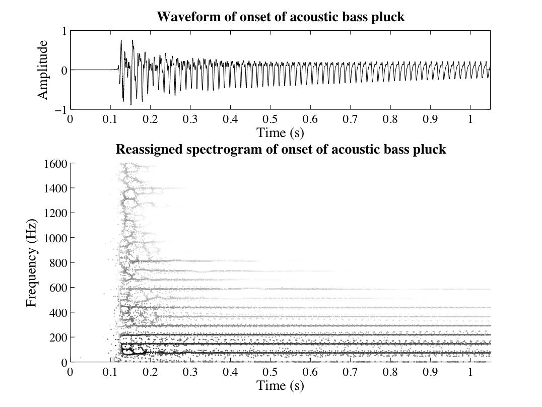
Figure 7: Reassigned spectrogram for the onset of an acoustic bass tone having a sharp pluck and a fundamental frequency of approximately 73.4 Hz. The spectrogram was computed using a 65.7 ms Kaiser window with a shaping parameter of 12. The sharp attack and the harmonic components are clearly visible.

In spite of the obvious gains in clarity, reassigned spectrograms can be disappointingly noisy. Seemingly random speckle is visible in regions where the reassigned data is not clearly associated with either a sinusoidal component or an impulsive component. This random speckle can be seen between the harmonics in Figure 7, and in the reassigned spectrogram shown in Figure 8, representing a portion of the vowel e (day), spoken in a “creaky” (low airflow) voice. The main glottal impulses appear as dark grey lines, and these result from the sudden release of a puff of air into the mouth from below the vocal cords. There are also fainter secondary impulses of unknown cause (these have been attributed to the mechanics of the vocal cord action), appearing just prior to the main impulses in this particular voice sample.

Reassignment provides a mapping from the geometrical center of the short-time analysis window to the center of gravity of a nearby dominant spectral component, but in low-energy regions of the spectrum, where there is no dominant component, data is reassigned in a way that has no apparent relationship to the structure of the analyzed signal.

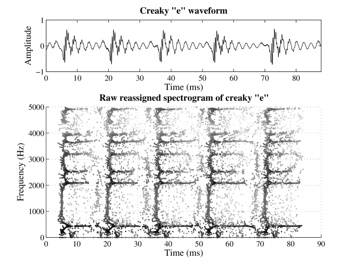
Figure 8: Reassigned spectrogram of the vowel e (day) computed using a 7.8 ms Hann window.

The reassignment operations can be used to gauge the quality or reliability of spectral analysis data. Large time or frequency reassignments indicate energy concentrated far from the geometrical center of the analysis window. Since window functions used in spectral analysis emphasize signal energy near their geometrical centers and de-emphasize signal energy far from their centers, large reassignments indicate data derived primarily from signal features that are not well-represented in a particular analysis window. Reassigned spectral data judged to be unreliable on the basis of large time reassignments [18] or large frequency reassignments [15] can be pruned from the representation to further improve its readability, with the assurance that, owing to the high redundancy of short-time Fourier transform data, the unreliable data will be represented more reliably in a neighboring short-time Fourier transform frame or channel. Gardner [15] further showed that consensus among neighboring estimates of reassigned frequency indicates that those frequency estimates are reliable, and therefore consensus can be used to guide the choice of an optimal analysis window for resolving sinusoidal components in spectrally sparse sounds.

When there is a high degree of consensus among reassigned frequency estimates, then the reassigned frequency, $\hat{\omega}(t,\omega)$ is changing very little with respect to the center frequency of the analysis window, that is

$$\frac{\partial\hat{\omega}(t,\omega)}{\partial\omega}\approx 0.$$ (104)

Since, from Equation 29, the reassigned frequency is computed from the partial derivative of spectral phase with respect to time, consensus among reassigned frequency estimates can be evaluated locally from the mixed partial derivative of spectral phase with respect to time and frequency. Specifically, in the vicinity of quasi-sinusoidal components, all frequencies, $\omega$, should be mapped to approximately the same reassigned frequency, $\hat{\omega}(t,\omega)$, so

$$\frac{\partial\hat{\omega}(t,\omega)}{\partial\omega}=1+\frac{\partial^{2}\phi(t,\omega)}{\partial t\partial\omega}\approx 0.$$ (105)

Nelson showed that the mixed partial derivative of spectral phase can be used to clean up or “de-speckle” reassigned spectrograms by removing data that does not correspond to strongly sinusoidal or impulsive components in the analyzed signal [10, 11]. By plotting just those points in a reassigned spectrogram meeting the condition on the mixed partial derivative expressed in Equation 105, a spectrogram showing just the strongly-sinusoidal components can be drawn. In a speech signal, analyzed using a short analysis window, these will be chiefly the vocal tract resonances. A reassigned spectrogram pruned in this way is shown in Figure 9 for the same speech signal plotted in Figure 8.

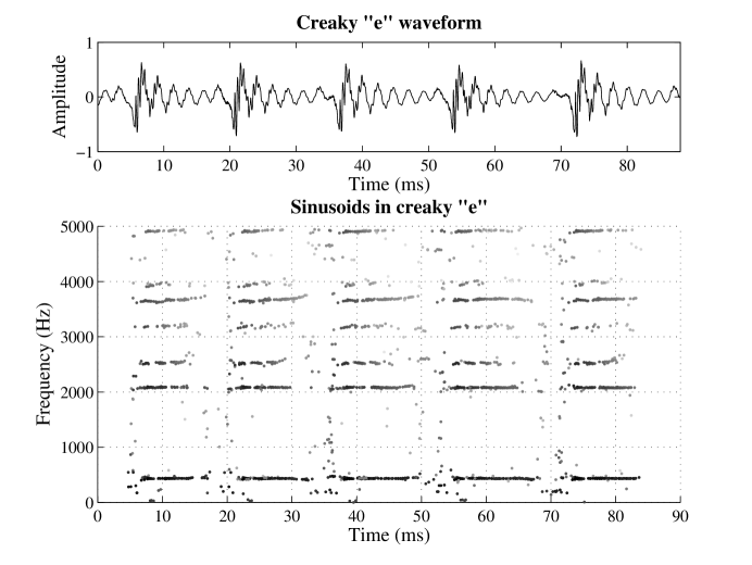
Figure 9: Reassigned spectrogram showing only the sinusoidal components in the vowel e (day). The spectrogram was computed using a 7.8 ms Hann window.

Nelson further demonstrated that impulsive components in a signal should be characterized by a high degree of consensus among neighboring reassigned time estimates. Near the time of the impulse, the reassigned time, $\hat{t}(t,\omega)$, should be changing very slowly with respect to the temporal center of the analysis window, that is,

$$\frac{\partial\hat{t}(t,\omega)}{\partial t}\approx 0.$$ (106)

Since, from Equation 28, the reassigned time is computed from the partial derivative of spectral phase with respect to frequency, consensus among reassigned time estimates can also be evaluated locally from the mixed partial derivative of spectral phase. In the vicinity of impulsive components, all times, $t$, should be mapped to approximately the same reassigned time, $\hat{t}(t,\omega)$, so

$$\frac{\partial\hat{t}(t,\omega)}{\partial\omega}=-\frac{\partial^{2}\phi(t,\omega)}{\partial t\partial\omega}\approx 0.$$ (107)

By plotting just those points in a reassigned spectrogram meeting the condition on the mixed partial derivative expressed in Equation 107, a spectrogram can be drawn that clearly and precisely localizes the impulsive events in a signal. For example, using a short (relative to the fundamental period) analysis window, the individual glottal pulses in a speech signal can be plotted, as shown for the creaky e signal in Figure 10.

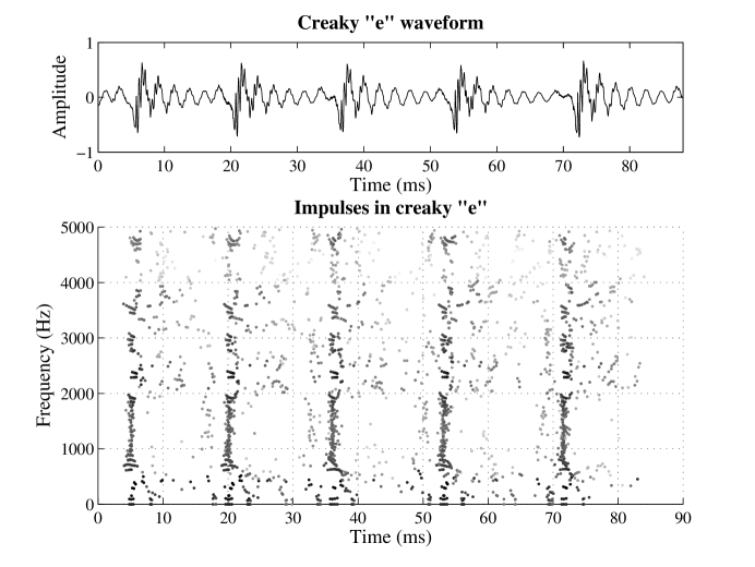
Figure 10: Reassigned spectrogram showing only the impulsive components in the vowel e (day). The spectrogram was computed using a 7.8 ms Hann window.

Using the phase of the moving window transform, Nelson identified the reassigned data corresponding to sinusoidal components as the points satisfying

$$\frac{\partial^{2}\phi_{t}(\omega)}{\partial t\partial\omega}\approx 0.$$ (108)

and the reassigned data corresponding to impulsive components as the points satisfying

$$\frac{\partial^{2}\phi_{t}(\omega)}{\partial t\partial\omega}\approx 1$$ (109)

Equations 108 and 109 are exactly equivalent to Equations 105 and 107, respectively; the apparent shift by one reflects the difference in spectral phase reported by the moving window transform and the short-time Fourier transform.

By plotting just those points in a reassigned spectrogram meeting the disjunction of these two conditions yields a “denoised” reassigned spectrogram showing precisely-localized quasi-sinusoidal and impulsive components, and excluding the objectionable “speckle”. Figure 11 shows a fully “despeckled” reassigned spectrogram of the creaky e, constructed solely from reassigned spectral data satisfying one of the conditions in Equations 105 and 107. Figure 12 shows a similarly “despeckled” reassigned spectrogram for the acoustic bass pluck shown in Figure 7.

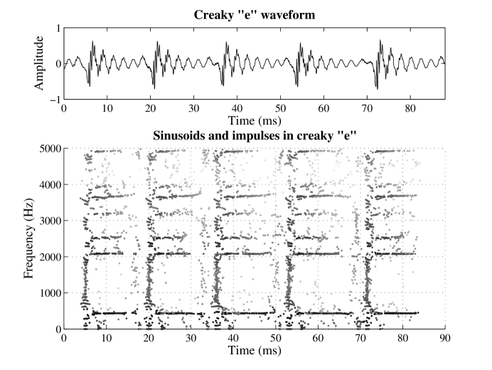
Figure 11: “Despeckled” reassigned spectrogram showing only the sinusoidal and impulsive components in the vowel e (day). The spectrogram was computed using a 7.8 ms Hann window.

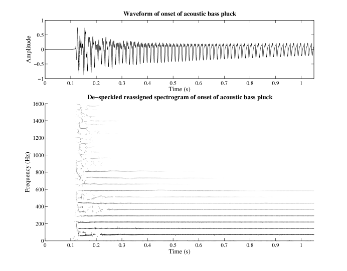
Figure 12: “Despeckled” reassigned spectrogram showing only the sinusoidal and impulsive components in the onset of an acoustic bass tone having a sharp pluck and a fundamental frequency of approximately 73.4 Hz. The spectrogram was computed using a 65.7 ms Kaiser window with a shaping parameter of 12.

Nelson used finite differences to compute the mixed partial derivative of spectral phase, but using the derivations of the reassignment operations in Sections 6.2.1 and 6.2.2, it can be shown the the mixed partial derivative can be computed directly from Fourier transforms by

$$\frac{\partial^{2}\phi(t,\omega)}{\partial t\partial\omega} =\Re\biggl{\{}\frac{X_{\mathcal{TD}h}(t,\omega)X^{\ast}(t,\omega)}{|X(t,\omega)|^{2}}\biggr{\}}-\Re\biggl{\{}\frac{X_{\mathcal{T}h}(t,\omega)X_{\mathcal{D}h}(t,\omega)}{X^{2}(t,\omega)}\biggr{\}}$$ (110)

where $X_{\mathcal{TD}h}(t,\omega)$ is the short-time Fourier transform of $x(t)$ computed using a window $h_{\mathcal{TD}}(t)=t\frac{d}{dt}h(t)$, that is, the window used to compute $X_{\mathcal{D}h}(t,\omega)$ multiplied by a time ramp.

8 Phase-Correct Additive Sound Modeling

In many applications, only the reassigned energy distribution is desired. In sound modeling applications, where the goal is to construct a model of the sound that can be used to reconstruct the sound, possibly with modifications, we retain not the squared magnitude of the Fourier transform, the spectrogram, but the magnitude and phase of the transform.

The reassigned bandwidth-enhanced additive sound model [24] is a high-fidelity representation that allows manipulations and transformations to be applied to a great variety of sounds, including noisy and non-harmonic sounds. It is similar in spirit to traditional sinusoidal models [6, 19, 25] in that a waveform is modeled as a collection of components, called partials, having time-varying frequencies and amplitudes. Estimates of partial frequency, amplitude, and phase are obtained by following ridges on a reassigned time-frequency surface, such as the one shown in Figure 13, constructed by reassigning discrete short-time Fourier transform data. This algorithm shares with traditional sinusoidal methods the notion of temporally-connected partial parameter estimates, but by contrast, the reassigned estimates are non-uniformly distributed in both time and frequency. The reassigned bandwidth-enhanced model yields greater resolution in time and frequency than is possible using conventional additive techniques, and can preserve the temporal envelope of transient signals, even in modified reconstruction, if the short-time phase information is properly maintained [18]. Preserving phase is important for reproducing transients and short-duration complex sounds having significant information in the temporal envelope [26].

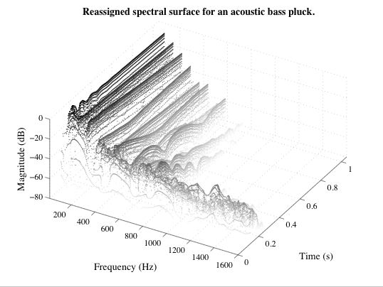
Figure 13: Reassigned spectral surface for the onset of an acoustic bass tone having a sharp pluck and a fundamental frequency of approximately 73.4 Hz. The spectrogram was computed using a 65.7 ms Kaiser window with a shaping parameter of 12.

The phase reported by the short-time Fourier transform is referenced to the geometrical center of the analysis window in time and frequency. For a sinusoid having instantaneous frequency equal to $\omega_{i}(t)$ (which is assumed to be slowly-varying with respect to time), the argument of the short-time Fourier transform evaluated at $t,\omega_{i}(t)$ will be precisely the phase of the sinusoid at time $t$. If the short-time Fourier transform is evaluated at some nearby frequency, $\omega_{i}(t)+\epsilon$, then the argument will not be precisely the phase of the sinusoid, because the transform is equivalent to the output of a bank of linear phase bandpass filters. These filters have phase equal to zero at the center of their passbands, so a sinusoid having frequency equal to the center frequency of the filter will see no phase shift, but a sinusoid having frequency not equal to the center frequency of the filter (but still in the passband) will experience a linear phase shift.

Frequency reassignment computes frequencies for discrete short-time Fourier transform data that are equal to the instantaneous frequency of the dominant component in the signal under analysis at each time and frequency at which the transform is evaluated, and attributes the data to these reassigned frequencies. Since the reassigned data represent energy in signal components having frequencies that are not at the geometrical center of the analysis window, it follows that the data is perturbed by a linear phase shift. This perturbation is easy to correct, because the slope of the phase response of the transform filters is known. In fact, since the phase is linear over the entire passband of the filter (this is why the finite difference approximation to the derivative is so accurate at points of significant energy, see section 6.1), the phase of reassigned short-time data can be corrected to agree with the reassigned frequency by linear interpolation of the discrete short-time phase spectrum.

Similarly, data that is reassigned in time away from the geometrical center of the analysis window needs to be corrected for the phase travel due to sinusoidal oscillation over the interval of time reassignment (that is, the interval between the reassigned time and the temporal center of the analysis window). In order to account for this phase travel precisely, the frequency trajectory must be known precisely. For many sounds, provided that the analysis window is not too long, the frequency can be assumed to be constant over the time reassignment interval, so a shift by $\hat{\omega}(t,\omega)\cdot\left[\hat{t}(t,\omega)-t\right]$ is sufficient to correct the phase of reassigned short-time data to agree with the reassigned time ($\hat{\omega}(t,\omega)$ is the reassigned instantaneous frequency and $\hat{t}(t,\omega)-t$ is time reassignment interval).

9 Computation of Higher-Order Phase Derivatives

The method of reassignment uses the partial derivatives of spectral phase with respect to time and frequency. Applications of higher-order partial derivatives of spectral phase have been proposed as well. Nelson showed that higher-order partial derivatives of phase could be approximated using cross-spectral surfaces [10, 11], but did not discuss any applications beyond the estimation of frequency slope, or chirp rate. Rihaczek [9] proposed that the second derivatives of the spectral phase be used to estimate the optimal dimensions of the time-frequency cells in a Gabor decomposition.

By methods similar to those described in Sections 6.2.1 and 6.2.2, it can be shown that the second partial derivative of phase with respect to frequency and time can be computed

$$\frac{\partial^{2}\phi(t,\omega)}{\partial\omega^{2}} =\Im\biggl{\{}\biggl{(}\frac{X_{\mathcal{T}h}(t,\omega)X^{\ast}(t,\omega)}{|X(t,\omega)|^{2}}\biggr{)}^{2}\biggr{\}}-\Im\biggl{\{}\frac{X_{\mathcal{T}^{2}h}(t,\omega)X^{\ast}(t,\omega)}{|X(t,\omega)|^{2}}\biggr{\}}$$ (111)

$$\frac{\partial^{2}\phi(t,\omega)}{\partial t^{2}} =\Im\biggl{\{}\frac{X_{\mathcal{D}^{2}h}(t,\omega)X^{\ast}(t,\omega)}{|X(t,\omega)|^{2}}\biggr{\}}-\Im\biggl{\{}\biggl{(}\frac{X_{\mathcal{D}h}(t,\omega)X^{\ast}(t,\omega)}{|X(t,\omega)|^{2}}\biggr{)}^{2}\biggr{\}}$$ (112)

where $X_{\mathcal{T}^{2}h}(t,\omega)$ is the short-time Fourier transform of $x(t)$ computed using a window $h_{\mathcal{T}^{2}}(t)=t^{2}h(t)$ and $X_{\mathcal{D}^{2}h}(t,\omega)$ is the short-time Fourier transform of $x(t)$ computed using a window $h_{\mathcal{D}^{2}}(t)=\frac{d^{2}}{dt^{2}}h(t)$.

We think that higher-order phase derivatives might be useful in computing local estimates of time and frequency spread that will allow us to construct more robust models of noisy sounds.

10 Conclusion

We have presented the theory of time-frequency reassignment in the context of the spectrogram, the most commonly-used time-frequency representation in speech and audio processing. Time-frequency reassignment sharpens blurry time-frequency data by relocating the data according to local estimates of instantaneous frequency and group delay. This mapping to reassigned time-frequency coordinates is very precise for signals that are separable in time and frequency with respect to the analysis window. We have discussed methods for computing reassigned times and frequencies in digital systems, and offered a derivation of one popular and efficient method. We believe that many speech and audio processing applications employing short-time spectral analysis could benefit from the straightforward application of the method of reassignment, and have discussed some examples from our own research. We further believe that extensions to the method of reassignment to efficiently compute mixed and higher-order spectral derivatives may provide a means of computing other features of interest in speech and audio signal processing.

Kelly Fitz received a Ph.D. in Electrical Engineering from the University of Illinois at Urbana-Champaign in 1999. He was the principle developer of the sound analysis and synthesis software Lemur, and, at the National Center for Supercomputing Applications, co-developer of the Vanilla Sound Server, an application providing real-time sound synthesis for virtual environments. Dr. Fitz is currently Assistant Professor of Electrical Engineering and Computer Science at Washington State University, and the principle developer of the Loris software for sound modeling and morphing. His research interests include speech and audio processing, digital sound synthesis, and computer music composition.

Sean A. Fulop was born in Calgary, Alberta, on 16 March 1970. He received a Ph.D. in linguistics from UCLA in 1999. After holding lectureships at San Jose State, the University of Chicago, and California State University Fresno, he became an Assistant Professor at Fresno in 2005. Dr. Fulop’s research interests include applications of new DSP methods in the analysis of speech and animal communication, as well as mathematical modeling of human language with the aid of computational learning theory and logic. Nonacademic interests include progressive rock music and nurturing an old sports car.

References

- [1] P. Flandrin, F. Auger, E. Chassande-Mottin, Time-frequency reassignment: From principles to algorithms, in: A. Papandreou-Suppappola (Ed.), Applications in Time-Frequency Signal Processing, CRC Press, 2003, Ch. 5, pp. 179 – 203.
- [2] S. Fulop, K. Fitz, Algorithms for computing the time-corrected instantaneous frequency (reassigned) spectrogram, with applications, Journal of the Acoustical Society of America (2005) to appear.
- [3] F. Auger, P. Flandrin, Improving the readability of time-frequency and time-scale representations by the reassignment method, IEEE Transactions on Signal Processing 43 (5) (1995) 1068 – 1089.
- [4] K. Kodera, R. Gendrin, C. de Villedary, Analysis of time-varying signals with small values, IEEE Transactions on Acoustics, Speech and Signal Processing ASSP-26 (1) (1978) 64 – 76.
- [5] M. Dolson, The phase vocoder: A tutorial, Computer Music Journal 10 (4) (1986) 14 – 27.
- [6] R. J. McAulay, T. F. Quatieri, Speech analysis/synthesis based on a sinusoidal representation, IEEE Transactions on Acoustics, Speech, and Signal Processing ASSP-34 (4) (1986) 744 – 754.
- [7] L. Cohen, Time-Frequency Analysis, Prentice-Hall, Englewood Cliffs, NJ, 1995.
- [8] A. Papoulis, Systems and Transforms with Applications to Optics, McGraw-Hill, New York, New York, 1968, Ch. 7.3, p. 234.
- [9] A. W. Rihaczek, Signal energy distribution in time and frequency, IEEE Transactions on Information Theory 4 (3) (1968) 369 – 374.
- [10] D. J. Nelson, Instantaneous higher order phase derivatives, Digital Signal Processing 12 (2 – 3) (2002) 416 – 428.
- [11] D. J. Nelson, Cross-spectral methods for processing speech, Journal of the Acoustical Society of America 110 (5) (2001) 2575 – 2592.
- [12] J. L. Flanagan, R. M. Golden, Phase vocoder, Bell System Technical Journal (1966) 1493 – 1509.
- [13] T. Nakatani, T. Irino, Robust and accurate fundamental frequency estimation based on dominant harmonic components, The Journal of the Acoustical Society of America 116 (6) (2004) 3690–3700.
- [14] M. Goto, A robust predominant-F0 estimation method for real-time detection of melody and bass lines in cd recordings, in: Proceedings of the IEEE International Conference on Acoustics, Speech, and Signal Processing, 2000, pp. II757 – II760.
- [15] T. J. Gardner, M. O. Magnasco, Instantaneous frequency decomposition: An application to spectrally sparse sounds with fast frequency modulations, The Journal of the Acoustical Society of America 117 (5) (2005) 2896–2903.
- [16] F. Plante, G. Meyer, W. A. Ainsworth, Improvement of speech spectrogram accuracy by the method of spectral reassignment, IEEE Transactions on Speech and Audio Processing 6 (3) (1998) 282 – 287.
- [17] S. Hainsworth, M. Macleod, P. Wolfe, Analysis of reassigned spectrograms for musical transcription, in: IEEE Workshop on the Applications of Signal Processing to Audio and Acoustics, 2001, pp. 23 – 26.
- [18] K. Fitz, L. Haken, On the use of time-frequency reassignment in additve sound modeling, Journal of the Audio Engineering Society 50 (11) (2002) 879 – 893.
- [19] X. Serra, J. O. Smith, Spectral modeling synthesis: A sound analysis/synthesis system based on a deterministic plus stochastic decomposition, Computer Music Journal 14 (4) (1990) 12 – 24.
- [20] F. Keiler, S. Marchand, Survey on extraction of sinusoids in stationary sounds, in: Proc. DAFx-02 Digital Audio Effects Conference, Hamburg, 2002, pp. 51–58.
- [21] F. Auger, P. Flandrin, The why and how of time-frequency reassignment, in: Proceedings of the IEEE-SP International Symposium on Time-Frequency and Time-Scale Analysis, 1994, pp. 197 – 200.
- [22] F. Charpentier, Pitch detection using the short-term phase spectrum, in: IEEE International Conference on Acoustics, Speech, and Signal Processing, Vol. 11, 1986, pp. 113 – 116.
- [23] T. Abe, T. Kobayashi, S. Imai, Robust pitch estimation with harmonics enhancement in noisy environments based on instantaneous frequency, in: Proceedings of the Fourth International Conference on Spoken Language, Vol. 2, 1996, pp. 1277 – 1280.
- [24] K. Fitz, L. Haken, S. Lefvert, C. Champion, M. O’Donnell, Cell-utes and flutter-tongued cats: Sound morphing using Loris and the reassigned bandwidth-enhanced model, Computer Music Journal 27 (4) (2003) 47 – 65.
- [25] K. Fitz, L. Haken, Sinusoidal modeling and manipulation using Lemur, Computer Music Journal 20 (4) (1996) 44 – 59.
- [26] T. F. Quatieri, R. B. Dunn, T. E. Hanna, Time-scale modification of complex acoustic signals, in: Proceedings of the International Conference on Acoustics, Speech, and Signal Processing, IEEE, 1993, pp. I–213 – I–216.