Low Temperature Science 68 (Suppl.), 137–148 (2009).
© Institute of Low Temperature Science, Hokkaido University, Sapporo, Japan.

Abstract: In order to study the mechanical behaviour of polar ice masses, the method of continuum mechanics is used. The newly developed CAFFE model (Continuum-mechanical, Anisotropic Flow model, based on an anisotropic Flow Enhancement factor) is described, which comprises an anisotropic flow law as well as a fabric evolution equation. The flow law is an extension of the isotropic Glen’s flow law, in which anisotropy enters via an enhancement factor that depends on the deformability of the polycrystal. The fabric evolution equation results from an orientational mass balance and includes constitutive relations for grain rotation and recrystallization. The CAFFE model fulfills all the fundamental principles of classical continuum mechanics, is sufficiently simple to allow numerical implementations in ice-flow models and contains only a limited number of free parameters. The applicability of the CAFFE model is demonstrated by a case study for the site of the EPICA (European Project for Ice Coring in Antarctica) ice core in Dronning Maud Land, East Antarctica.

Key words: Ice, polycrystal, flow, anisotropy, continuum mechanics, ice core

1 Introduction

Ice in natural land ice masses, such as polar ice sheets, ice caps or glaciers, consists of zillions of individual hexagonal crystals (“crystallites” or “grains”) with a typical diameter of millimeters to centimeters. This length scale stands in contrast with the size of the ice masses, which ranges from 100’s of meters to 1000’s of kilometers. It has long been known that, while the distribution of the crystallographic axes (also known as optical axes or $c$-axes) at the surface of an ice sheet is essentially at random, deeper down into the ice, different types of anisotropic fabrics with preferred orientations of the $c$-axes tend to develop.

Many models have been proposed to describe the anisotropy of polar ice. On the one end of the range in complexity, a simple flow enhancement factor is introduced in an ad-hoc fashion as a multiplier of the isotropic ice fluidity in order to account for anisotropy and/or impurities. This is done in most current ice-sheet models, often without explicitly mentioning anisotropy [19, 25, 46]. In macroscopic, phenomenological models, an anisotropic macroscopic formulation for the flow law of the polycrystal is postulated. To be usable, the rheological parameters that enter this law must be evaluated as functions of the anisotropic fabric [14, 15, 34, 35]. The concept of homogenization models, also called micro-macro models, is to derive the polycrystalline behaviour at the level of individual crystals and the fabric [1, 4, 5, 17, 26, 29, 50, 51]. As for the “high-end” complexity, full-field models solve the Stokes equation for ice flow properly by decomposing the polycrystal into many elements, which makes it possible to infer the stress and strain-rate heterogeneities at the microscopic scale [27, 28, 30, 31]. A very comprehensive, up-to-date overview of these different types of models is given by Gagliardini et al. [13] (in this volume). However, the more sophisticated models are usually too complex and computationally time-consuming to be included readily in a model of macroscopic ice flow.

Here, the Continuum-mechanical, Anisotropic Flow model, based on an anisotropic Flow Enhancement factor (“CAFFE model”), shall be described. It belongs to the class of macroscopic models, and is laid down in detail in the study by Placidi et al. [42] (based on previous works by Faria [10, 11], Faria et al. [12], Placidi [40, 41], Placidi and Hutter [43]). The flow enhancement factor is taken as a function of a newly introduced scalar quantity called deformability, which is essentially a non-dimensional invariant related to the shear stress acting on the basal plane of a crystallite, weighted by the orientation-distribution function which describes the anisotropic fabric of the polycrystal. Fabric evolution is modelled by an orientation mass balance which accounts for grain rotation and recrystallization processes.

The CAFFE model fulfills all the fundamental principles of classical continuum mechanics (see also Placidi et al. [44]), and it is a good compromise between necessary simplicity on the one hand, and consideration of the major effects of anisotropy on the other. In order to demonstrate its performance, the model is applied to the site of the EPICA (European Project for Ice Coring in Antarctica) ice core in Dronning Maud Land, East Antarctica, for which data on the ice flow as well as on the anisotropic fabric are available.

2 CAFFE model

2.1 Glen’s flow law

Quantity	Value
Stress exponent, $n$	$3$
Pre-exponential constant, $A_{0}$	$\begin{array}[t]{ll}3.985\times{}10^{-13}\,\mathrm{s^{-1}\,Pa^{-3}}&\mbox{(for $T^{\prime}\leq{}263.15\,\mathrm{K}$)}\\ 1.916\times{}10^{3}\,\mathrm{s^{-1}\,Pa^{-3}}&\mbox{(for $T^{\prime}>263.15\,\mathrm{K}$)}\end{array}$
Activation energy, $Q$	$\begin{array}[t]{ll}60\,\mathrm{kJ\,mol^{-1}}&\hskip 44.0pt\mbox{(for $T^{\prime}\leq{}263.15\,\mathrm{K}$)}\\ 139\,\mathrm{kJ\,mol^{-1}}&\hskip 44.0pt\mbox{(for $T^{\prime}>263.15\,\mathrm{K}$)}\end{array}$

Table 1: Physical parameters for Glen’s flow law.

Let us briefly review the isotropic case, for which polycrystalline ice is treated as an incompressible, viscous fluid. The Cauchy stress tensor $\sf\textstyle T$ is split up according to

$$\mathchoice{\mbox{$\sf\displaystyle T$}}{\mbox{$\sf\textstyle T$}}{\mbox{$\sf\scriptstyle T$}}{\mbox{$\sf\scriptscriptstyle T$}}=-p\mathchoice{\mbox{$\sf\displaystyle 1$}}{\mbox{$\sf\textstyle 1$}}{\mbox{$\sf\scriptstyle 1$}}{\mbox{$\sf\scriptscriptstyle 1$}}+\mathchoice{\mbox{$\sf\displaystyle S$}}{\mbox{$\sf\textstyle S$}}{\mbox{$\sf\scriptstyle S$}}{\mbox{$\sf\scriptscriptstyle S$}},\qquad p=-\frac{1}{3}\mbox{tr}\,\mathchoice{\mbox{$\sf\displaystyle T$}}{\mbox{$\sf\textstyle T$}}{\mbox{$\sf\scriptstyle T$}}{\mbox{$\sf\scriptscriptstyle T$}},$$ (1)

where $p$ denotes the pressure, and $\sf\textstyle S$ is the traceless stress deviator ($\mbox{tr}\,\mathchoice{\mbox{$\sf\displaystyle S$}}{\mbox{$\sf\textstyle S$}}{\mbox{$\sf\scriptstyle S$}}{\mbox{$\sf\scriptscriptstyle S$}}=0$). Due to the incompressibility, the flow law only determines the stress deviator $\sf\textstyle S$ and reads

$$\mathchoice{\mbox{$\sf\displaystyle S$}}{\mbox{$\sf\textstyle S$}}{\mbox{$\sf\scriptstyle S$}}{\mbox{$\sf\scriptscriptstyle S$}}=2\eta\mathchoice{\mbox{$\sf\displaystyle D$}}{\mbox{$\sf\textstyle D$}}{\mbox{$\sf\scriptstyle D$}}{\mbox{$\sf\scriptscriptstyle D$}},$$ (2)

where $\mathchoice{\mbox{$\sf\displaystyle D$}}{\mbox{$\sf\textstyle D$}}{\mbox{$\sf\scriptstyle D$}}{\mbox{$\sf\scriptscriptstyle D$}}=\mbox{sym}\,\mbox{grad}\,\mathchoice{\mbox{\boldmath$\bf\displaystyle v$}}{\mbox{\boldmath$\bf\textstyle v$}}{\mbox{\boldmath$\bf\scriptstyle v$}}{\mbox{\boldmath$\bf\scriptscriptstyle v$}}$ is the strain-rate tensor (symmetric part of the gradient of the velocity $\bf\textstyle v$), and the coefficient $\eta$ is the shear viscosity (or simply the viscosity). Its inverse, the fluidity, can be factorized as

$$\frac{1}{\eta}=2EA(T^{\prime})f(\sigma),$$ (3)

where

$$\sigma=\sqrt{\mbox{$\frac{1}{2}$}\,\mbox{tr}\,(\mathchoice{\mbox{$\sf\displaystyle S$}}{\mbox{$\sf\textstyle S$}}{\mbox{$\sf\scriptstyle S$}}{\mbox{$\sf\scriptscriptstyle S$}}^{2})}$$ (4)

is the effective stress (square root of the second invariant of the stress deviator), and the creep function $f(\sigma)$ is given by the power law

$$f(\sigma)=\sigma^{n-1}$$ (5)

(the parameter $n$ is called “stress exponent”). Further, the rate factor $A(T^{\prime})$ depends on the temperature relative to pressure melting $T^{\prime}=T-T_{\mathrm{m}}+T_{0}$ ($T$: absolute temperature, $T_{\mathrm{m}}=T_{0}-\beta{}p\,$: pressure melting point, $T_{0}=273.16\,\mathrm{K}\,$: melting point at zero pressure, $\beta=9.8\times{}10^{-2}\,\mathrm{K\,MPa^{-1}}$: Clausius-Clapeyron constant) via the Arrhenius law

$$A(T^{\prime})=A_{0}\,e^{-Q/RT^{\prime}},$$ (6)

where $A_{0}$ is the pre-exponential constant, $Q$ the activation energy and $R=8.314\,\mathrm{J\,mol^{-1}\,K^{-1}}$ the universal gas constant. The flow enhancement factor $E$ is equal to unity for pure ice, and can be set to values deviating from unity in order to account roughly for effects of impurities and/or anisotropy (Paterson [37]).

The isotropic flow law for ice is now obtained by inserting Eq. (3) [with the specifications of Eqs. (5) and (6)] in the viscous flow law (2). This yields

$$\mathchoice{\mbox{$\sf\displaystyle D$}}{\mbox{$\sf\textstyle D$}}{\mbox{$\sf\scriptstyle D$}}{\mbox{$\sf\scriptscriptstyle D$}}=EA(T^{\prime})f(\sigma)\,\mathchoice{\mbox{$\sf\displaystyle S$}}{\mbox{$\sf\textstyle S$}}{\mbox{$\sf\scriptstyle S$}}{\mbox{$\sf\scriptscriptstyle S$}},$$ (7)

which is called Nye’s generalization of Glen’s flow law, or Glen’s flow law for short (e.g., Greve and Blatter [20], Hooke [23], Paterson [38], van der Veen [52]). Suitable values for the several parameters are listed in Table 1.

2.2 Anisotropic generalization of Glen’s flow law

2.2.1 Deformation of a crystallite

In order to derive a generalization of Glen’s flow law (7) which accounts for general, anisotropic fabrics of the ice polycrystal, we first consider the deformation of a crystallite embedded in the polycrystalline aggregate. Following Placidi et al. [42], only the dominant deformation along the basal plane is accounted for, whereas deformations along prismatic and pyramidal planes, which are at least 60 times more difficult to activate, shall be neglected (Fig. 2.2.1).

Figure 1: Basal, prismatic and pyramidal glide planes in the hexagonal ice crystal, sketched as a right hexagonal prism (Faria [9]).

Let $\bf\textstyle n$ be the normal unit vector of the basal plane (direction of the $c$-axis), then $\sf\textstyle T$$\bf\textstyle n$ is the resolved stress vector (Fig. 2.2.1). Note that the tensor $\sf\textstyle T$ is interpreted as the macroscopic stress which does not depend on the orientation $\bf\textstyle n$. It is reasonable to assume that only the stress component $S_{\mathrm{t}}$ tangential to the basal plane (resolved shear stress) contributes to its shear deformation, while the component normal to the basal plane has no effect.

Figure 2: Decomposition of the stress vector into a part normal and a part tangential to the basal plane.

According to Fig. 2.2.1, the decomposition of the stress vector reads

$$\mathchoice{\mbox{$\sf\displaystyle T$}}{\mbox{$\sf\textstyle T$}}{\mbox{$\sf\scriptstyle T$}}{\mbox{$\sf\scriptscriptstyle T$}}\mathchoice{\mbox{\boldmath$\bf\displaystyle n$}}{\mbox{\boldmath$\bf\textstyle n$}}{\mbox{\boldmath$\bf\scriptstyle n$}}{\mbox{\boldmath$\bf\scriptscriptstyle n$}}=(\mathchoice{\mbox{$\sf\displaystyle T$}}{\mbox{$\sf\textstyle T$}}{\mbox{$\sf\scriptstyle T$}}{\mbox{$\sf\scriptscriptstyle T$}}\mathchoice{\mbox{\boldmath$\bf\displaystyle n$}}{\mbox{\boldmath$\bf\textstyle n$}}{\mbox{\boldmath$\bf\scriptstyle n$}}{\mbox{\boldmath$\bf\scriptscriptstyle n$}}\cdot\mathchoice{\mbox{\boldmath$\bf\displaystyle n$}}{\mbox{\boldmath$\bf\textstyle n$}}{\mbox{\boldmath$\bf\scriptstyle n$}}{\mbox{\boldmath$\bf\scriptscriptstyle n$}})\mathchoice{\mbox{\boldmath$\bf\displaystyle n$}}{\mbox{\boldmath$\bf\textstyle n$}}{\mbox{\boldmath$\bf\scriptstyle n$}}{\mbox{\boldmath$\bf\scriptscriptstyle n$}}+S_{\mathrm{t}}\mathchoice{\mbox{\boldmath$\bf\displaystyle t$}}{\mbox{\boldmath$\bf\textstyle t$}}{\mbox{\boldmath$\bf\scriptstyle t$}}{\mbox{\boldmath$\bf\scriptscriptstyle t$}},$$ (8)

where $\bf\textstyle t$ denotes the tangential unit vector. Inserting the decomposition (1) of the stress tensor $\sf\textstyle T$ readily eliminates the pressure $p$ and leaves

$$\mathchoice{\mbox{$\sf\displaystyle S$}}{\mbox{$\sf\textstyle S$}}{\mbox{$\sf\scriptstyle S$}}{\mbox{$\sf\scriptscriptstyle S$}}\mathchoice{\mbox{\boldmath$\bf\displaystyle n$}}{\mbox{\boldmath$\bf\textstyle n$}}{\mbox{\boldmath$\bf\scriptstyle n$}}{\mbox{\boldmath$\bf\scriptscriptstyle n$}}=(\mathchoice{\mbox{$\sf\displaystyle S$}}{\mbox{$\sf\textstyle S$}}{\mbox{$\sf\scriptstyle S$}}{\mbox{$\sf\scriptscriptstyle S$}}\mathchoice{\mbox{\boldmath$\bf\displaystyle n$}}{\mbox{\boldmath$\bf\textstyle n$}}{\mbox{\boldmath$\bf\scriptstyle n$}}{\mbox{\boldmath$\bf\scriptscriptstyle n$}}\cdot\mathchoice{\mbox{\boldmath$\bf\displaystyle n$}}{\mbox{\boldmath$\bf\textstyle n$}}{\mbox{\boldmath$\bf\scriptstyle n$}}{\mbox{\boldmath$\bf\scriptscriptstyle n$}})\mathchoice{\mbox{\boldmath$\bf\displaystyle n$}}{\mbox{\boldmath$\bf\textstyle n$}}{\mbox{\boldmath$\bf\scriptstyle n$}}{\mbox{\boldmath$\bf\scriptscriptstyle n$}}+S_{\mathrm{t}}\mathchoice{\mbox{\boldmath$\bf\displaystyle t$}}{\mbox{\boldmath$\bf\textstyle t$}}{\mbox{\boldmath$\bf\scriptstyle t$}}{\mbox{\boldmath$\bf\scriptscriptstyle t$}}.$$ (9)

As mentioned above, deformation of the crystallite in the polycrystalline aggregate is attributed to the tangential component $S_{\mathrm{t}}$ only. Since we aim at a theory which describes the effects of anisotropy by a scalar, anisotropic flow enhancement factor, we define the scalar invariant

$$S_{\mathrm{t}}^{2}=\mathchoice{\mbox{$\sf\displaystyle S$}}{\mbox{$\sf\textstyle S$}}{\mbox{$\sf\scriptstyle S$}}{\mbox{$\sf\scriptscriptstyle S$}}\mathchoice{\mbox{\boldmath$\bf\displaystyle n$}}{\mbox{\boldmath$\bf\textstyle n$}}{\mbox{\boldmath$\bf\scriptstyle n$}}{\mbox{\boldmath$\bf\scriptscriptstyle n$}}\cdot\mathchoice{\mbox{$\sf\displaystyle S$}}{\mbox{$\sf\textstyle S$}}{\mbox{$\sf\scriptstyle S$}}{\mbox{$\sf\scriptscriptstyle S$}}\mathchoice{\mbox{\boldmath$\bf\displaystyle n$}}{\mbox{\boldmath$\bf\textstyle n$}}{\mbox{\boldmath$\bf\scriptstyle n$}}{\mbox{\boldmath$\bf\scriptscriptstyle n$}}-(\mathchoice{\mbox{$\sf\displaystyle S$}}{\mbox{$\sf\textstyle S$}}{\mbox{$\sf\scriptstyle S$}}{\mbox{$\sf\scriptscriptstyle S$}}\mathchoice{\mbox{\boldmath$\bf\displaystyle n$}}{\mbox{\boldmath$\bf\textstyle n$}}{\mbox{\boldmath$\bf\scriptstyle n$}}{\mbox{\boldmath$\bf\scriptscriptstyle n$}}\cdot\mathchoice{\mbox{\boldmath$\bf\displaystyle n$}}{\mbox{\boldmath$\bf\textstyle n$}}{\mbox{\boldmath$\bf\scriptstyle n$}}{\mbox{\boldmath$\bf\scriptscriptstyle n$}})^{2}.$$ (10)

This quantity has the unit of a stress squared, and so a natural way to non-dimensionalize it is by the square of the effective stress $\sigma$ [Eq. (4)], which is also a scalar invariant. Thus, we introduce the deformability of a crystallite in the polycrystalline aggregate, which is loaded by the stress $\sf\textstyle T$, as

$$\mathcal{A}^{\star}(\mathchoice{\mbox{\boldmath$\bf\displaystyle n$}}{\mbox{\boldmath$\bf\textstyle n$}}{\mbox{\boldmath$\bf\scriptstyle n$}}{\mbox{\boldmath$\bf\scriptscriptstyle n$}})=\frac{5}{2}\,\frac{S_{\mathrm{t}}^{2}(\mathchoice{\mbox{\boldmath$\bf\displaystyle n$}}{\mbox{\boldmath$\bf\textstyle n$}}{\mbox{\boldmath$\bf\scriptstyle n$}}{\mbox{\boldmath$\bf\scriptscriptstyle n$}})}{\sigma^{2}}=5\,\frac{\mathchoice{\mbox{$\sf\displaystyle S$}}{\mbox{$\sf\textstyle S$}}{\mbox{$\sf\scriptstyle S$}}{\mbox{$\sf\scriptscriptstyle S$}}\mathchoice{\mbox{\boldmath$\bf\displaystyle n$}}{\mbox{\boldmath$\bf\textstyle n$}}{\mbox{\boldmath$\bf\scriptstyle n$}}{\mbox{\boldmath$\bf\scriptscriptstyle n$}}\cdot\mathchoice{\mbox{$\sf\displaystyle S$}}{\mbox{$\sf\textstyle S$}}{\mbox{$\sf\scriptstyle S$}}{\mbox{$\sf\scriptscriptstyle S$}}\mathchoice{\mbox{\boldmath$\bf\displaystyle n$}}{\mbox{\boldmath$\bf\textstyle n$}}{\mbox{\boldmath$\bf\scriptstyle n$}}{\mbox{\boldmath$\bf\scriptscriptstyle n$}}-(\mathchoice{\mbox{$\sf\displaystyle S$}}{\mbox{$\sf\textstyle S$}}{\mbox{$\sf\scriptstyle S$}}{\mbox{$\sf\scriptscriptstyle S$}}\mathchoice{\mbox{\boldmath$\bf\displaystyle n$}}{\mbox{\boldmath$\bf\textstyle n$}}{\mbox{\boldmath$\bf\scriptstyle n$}}{\mbox{\boldmath$\bf\scriptscriptstyle n$}}\cdot\mathchoice{\mbox{\boldmath$\bf\displaystyle n$}}{\mbox{\boldmath$\bf\textstyle n$}}{\mbox{\boldmath$\bf\scriptstyle n$}}{\mbox{\boldmath$\bf\scriptscriptstyle n$}})^{2}}{\mbox{tr}\,(\mathchoice{\mbox{$\sf\displaystyle S$}}{\mbox{$\sf\textstyle S$}}{\mbox{$\sf\scriptstyle S$}}{\mbox{$\sf\scriptscriptstyle S$}}^{2})}.$$ (11)

The factor $5/2$ has been introduced merely for reasons of convenience, as it will become clear below.

2.2.2 Flow law for polycrystalline ice

In polycrystalline ice, the crystallites within a control volume (which is assumed to be large compared to the crystallite dimensions, but small compared to the macroscopic scale of ice flow) show a certain fabric. Extreme cases are on the one hand the single maximum fabric, for which all $c$-axes are perfectly aligned, and on the other hand the isotropic fabric with a completely random distribution of the $c$-axes. A general fabric, which is usually in between these cases, can be described by the orientation mass density (OMD) $\rho^{\star}(\mathchoice{\mbox{\boldmath$\bf\displaystyle n$}}{\mbox{\boldmath$\bf\textstyle n$}}{\mbox{\boldmath$\bf\scriptstyle n$}}{\mbox{\boldmath$\bf\scriptscriptstyle n$}})$. It is defined as the mass per volume and orientation, the latter being specified by the normal unit vector (direction of the $c$-axis) $\mathchoice{\mbox{\boldmath$\bf\displaystyle n$}}{\mbox{\boldmath$\bf\textstyle n$}}{\mbox{\boldmath$\bf\scriptstyle n$}}{\mbox{\boldmath$\bf\scriptscriptstyle n$}}\in{}S^{2}$ ($S^{2}$ is the unit sphere). Evidently, when integrated over all orientations, the OMD must yield the normal mass density $\rho$, which leads to the normalization condition

$$\int\limits_{S^{2}}\rho^{\star}(\mathchoice{\mbox{\boldmath$\bf\displaystyle n$}}{\mbox{\boldmath$\bf\textstyle n$}}{\mbox{\boldmath$\bf\scriptstyle n$}}{\mbox{\boldmath$\bf\scriptscriptstyle n$}})\,\mathrm{d}^{2}n=\rho.$$ (12)

Alternatively, an orientation distribution function (ODF) $f^{\star}(\mathchoice{\mbox{\boldmath$\bf\displaystyle n$}}{\mbox{\boldmath$\bf\textstyle n$}}{\mbox{\boldmath$\bf\scriptstyle n$}}{\mbox{\boldmath$\bf\scriptscriptstyle n$}})$ can be defined as

$$f^{\star}(\mathchoice{\mbox{\boldmath$\bf\displaystyle n$}}{\mbox{\boldmath$\bf\textstyle n$}}{\mbox{\boldmath$\bf\scriptstyle n$}}{\mbox{\boldmath$\bf\scriptscriptstyle n$}})=\frac{\rho^{\star}(\mathchoice{\mbox{\boldmath$\bf\displaystyle n$}}{\mbox{\boldmath$\bf\textstyle n$}}{\mbox{\boldmath$\bf\scriptstyle n$}}{\mbox{\boldmath$\bf\scriptscriptstyle n$}})}{\rho},$$ (13)

which is normalized to unity when integrated over all orientations.

We use the ODF in order to define the deformability of polycrystalline ice by weighting the deformability of the crystallite (11),

$$\mathcal{A} \!\!\!=\!\!\! \int\limits_{S^{2}}\mathcal{A}^{\star}(\mathchoice{\mbox{\boldmath$\bf\displaystyle n$}}{\mbox{\boldmath$\bf\textstyle n$}}{\mbox{\boldmath$\bf\scriptstyle n$}}{\mbox{\boldmath$\bf\scriptscriptstyle n$}})\,f^{\star}(\mathchoice{\mbox{\boldmath$\bf\displaystyle n$}}{\mbox{\boldmath$\bf\textstyle n$}}{\mbox{\boldmath$\bf\scriptstyle n$}}{\mbox{\boldmath$\bf\scriptscriptstyle n$}})\,\mathrm{d}^{2}n$$ (14)

$$\!\!\!=\!\!\! \frac{5}{2}\int\limits_{S^{2}}\frac{S_{\mathrm{t}}^{2}(\mathchoice{\mbox{\boldmath$\bf\displaystyle n$}}{\mbox{\boldmath$\bf\textstyle n$}}{\mbox{\boldmath$\bf\scriptstyle n$}}{\mbox{\boldmath$\bf\scriptscriptstyle n$}})}{\sigma^{2}}f^{\star}(\mathchoice{\mbox{\boldmath$\bf\displaystyle n$}}{\mbox{\boldmath$\bf\textstyle n$}}{\mbox{\boldmath$\bf\scriptstyle n$}}{\mbox{\boldmath$\bf\scriptscriptstyle n$}})\,\mathrm{d}^{2}n$$

$$\!\!\!=\!\!\! 5\int\limits_{S^{2}}\frac{\mathchoice{\mbox{$\sf\displaystyle S$}}{\mbox{$\sf\textstyle S$}}{\mbox{$\sf\scriptstyle S$}}{\mbox{$\sf\scriptscriptstyle S$}}\mathchoice{\mbox{\boldmath$\bf\displaystyle n$}}{\mbox{\boldmath$\bf\textstyle n$}}{\mbox{\boldmath$\bf\scriptstyle n$}}{\mbox{\boldmath$\bf\scriptscriptstyle n$}}\cdot\mathchoice{\mbox{$\sf\displaystyle S$}}{\mbox{$\sf\textstyle S$}}{\mbox{$\sf\scriptstyle S$}}{\mbox{$\sf\scriptscriptstyle S$}}\mathchoice{\mbox{\boldmath$\bf\displaystyle n$}}{\mbox{\boldmath$\bf\textstyle n$}}{\mbox{\boldmath$\bf\scriptstyle n$}}{\mbox{\boldmath$\bf\scriptscriptstyle n$}}-(\mathchoice{\mbox{$\sf\displaystyle S$}}{\mbox{$\sf\textstyle S$}}{\mbox{$\sf\scriptstyle S$}}{\mbox{$\sf\scriptscriptstyle S$}}\mathchoice{\mbox{\boldmath$\bf\displaystyle n$}}{\mbox{\boldmath$\bf\textstyle n$}}{\mbox{\boldmath$\bf\scriptstyle n$}}{\mbox{\boldmath$\bf\scriptscriptstyle n$}}\cdot\mathchoice{\mbox{\boldmath$\bf\displaystyle n$}}{\mbox{\boldmath$\bf\textstyle n$}}{\mbox{\boldmath$\bf\scriptstyle n$}}{\mbox{\boldmath$\bf\scriptscriptstyle n$}})^{2}}{\mbox{tr}\,(\mathchoice{\mbox{$\sf\displaystyle S$}}{\mbox{$\sf\textstyle S$}}{\mbox{$\sf\scriptstyle S$}}{\mbox{$\sf\scriptscriptstyle S$}}^{2})}f^{\star}(\mathchoice{\mbox{\boldmath$\bf\displaystyle n$}}{\mbox{\boldmath$\bf\textstyle n$}}{\mbox{\boldmath$\bf\scriptstyle n$}}{\mbox{\boldmath$\bf\scriptscriptstyle n$}})\,\mathrm{d}^{2}n.$$

Note that, for the isotropic case, the ODF is $f^{\star}(\mathchoice{\mbox{\boldmath$\bf\displaystyle n$}}{\mbox{\boldmath$\bf\textstyle n$}}{\mbox{\boldmath$\bf\scriptstyle n$}}{\mbox{\boldmath$\bf\scriptscriptstyle n$}})=1/(4\pi)$, and from Eq. (14) we obtain a deformability of $\mathcal{A}=1$ (Placidi et al. [42]). For that reason, the factor $5/2$ has been introduced in Eq. (11).

Figure 3: Uniaxial compression on single maximum (UC/SM) and simple shear on single maximum (SS/SM) for a small sample of polycrystalline ice. Stresses are indicated as black arrows, and the single maximum fabric is marked by the dark-grey arrows within the ice sample.

The envisaged flow law for anisotropic polar ice can now be formulated. Essentially, we keep the form of the Glen’s flow law (7), but with a scalar, anisotropic enhancement factor $\hat{E}(\mathcal{A})$ instead of the parameter $E$,

$$\mathchoice{\mbox{$\sf\displaystyle D$}}{\mbox{$\sf\textstyle D$}}{\mbox{$\sf\scriptstyle D$}}{\mbox{$\sf\scriptscriptstyle D$}}=\hat{E}(\mathcal{A})\,A(T^{\prime})f(\sigma)\,\mathchoice{\mbox{$\sf\displaystyle S$}}{\mbox{$\sf\textstyle S$}}{\mbox{$\sf\scriptstyle S$}}{\mbox{$\sf\scriptscriptstyle S$}}.$$ (15)

The function $\hat{E}(\mathcal{A})$ is supposed to be strictly increasing with the deformability $\mathcal{A}$, and has the fixed points

$$\begin{array}[]{l}\hat{E}(0)=E_{\mathrm{min}}\\[4.30554pt] \;\;\;\mbox{(uniaxial compression on single maximum)},\\[4.30554pt] \hat{E}(1)=1\\[4.30554pt] \;\;\;\mbox{(arbitrary stress on isotropic fabric)},\\[4.30554pt] \hat{E}(\frac{5}{2})=E_{\mathrm{max}}\\[4.30554pt] \;\;\;\mbox{(simple shear on single maximum)}.\end{array}$$ (16)

The “hard” case (16)₁ and the “soft” case (16)₃ are illustrated in Fig. 2.2.2. Note also that the deformability cannot take values larger than $\mathcal{A}=5/2$ (Placidi et al. [42]).

For the detailed form $\hat{E}(\mathcal{A})$ of the anisotropic enhancement factor, in addition to Eq. (16), we demand that the function is continuously differentiable, that is, $\hat{E}\in{}C^{1}[0,\frac{5}{2}]$. Moreover, Azuma [2] and Miyamoto [32] have experimentally verified that the enhancement factor depends on the Schmid factor (resolved shear stress) to the fourth power, that is, on the square of the deformability $\mathcal{A}$. This yields

$$\hat{E}(\mathcal{A})=\left\{\begin{array}[]{l}E_{\mathrm{min}}+(1-E_{\mathrm{min}})\mathcal{A}^{t},\\[12.91663pt] \hskip 35.00005ptt=\mbox{$\displaystyle\frac{8}{21}$}\,\mbox{$\displaystyle\frac{E_{\mathrm{max}}-1}{1-E_{\mathrm{min}}}$},\\[12.91663pt] \hskip 90.00014pt0\leq\mathcal{A}\leq 1,\\[12.91663pt] \mbox{$\displaystyle\frac{4\mathcal{A}^{2}(E_{\mathrm{max}}-1)+25-4E_{\mathrm{max}}}{21}$},\\[12.91663pt] \hskip 90.00014pt1\leq\mathcal{A}\leq\mbox{$\displaystyle\frac{5}{2}$}\end{array}\right.$$ (17)

(for details see Placidi et al. [42]). Several investigations (e.g. Budd and Jacka [3], Pimienta et al. [39], Russell-Head and Budd [45]) indicate that the parameter $E_{\mathrm{max}}$ (maximum softening) is approximately equal to ten. The parameter $E_{\mathrm{min}}$ (maximum hardening) can be realistically chosen between zero and one tenth, a non-zero value serving mainly the purpose of avoiding numerical problems. The function (17) is shown in Fig. 2.2.2.

Figure 4: Anisotropic enhancement factor $\hat{E}(\mathcal{A})$ as a function of the deformability $\mathcal{A}$ according to Eq. (17), for $E_{\mathrm{max}}=10$ and $E_{\mathrm{min}}=0$.

2.2.3 Inversion of the flow law

As long as the creep function $f(\sigma)$ is given by the power law (5), the anisotropic flow law (15) can be inverted analytically. We find

$$\mathchoice{\mbox{$\sf\displaystyle S$}}{\mbox{$\sf\textstyle S$}}{\mbox{$\sf\scriptstyle S$}}{\mbox{$\sf\scriptscriptstyle S$}}=[\hat{E}(\mathcal{A})]^{-1/n}\,[A(T^{\prime})]^{-1/n}\,d^{-(1-1/n)}\,\mathchoice{\mbox{$\sf\displaystyle D$}}{\mbox{$\sf\textstyle D$}}{\mbox{$\sf\scriptstyle D$}}{\mbox{$\sf\scriptscriptstyle D$}},$$ (18)

where

$$d=\sqrt{\mbox{$\frac{1}{2}$}\,\mbox{tr}\,(\mathchoice{\mbox{$\sf\displaystyle D$}}{\mbox{$\sf\textstyle D$}}{\mbox{$\sf\scriptstyle D$}}{\mbox{$\sf\scriptscriptstyle D$}}^{2})}$$ (19)

is the effective strain rate. The deformability $\mathcal{A}$ also needs to be expressed by strain rates instead of stresses [see Eq. (14)]. In analogy to Eq. (9), we consider the resolved strain-rate vector $\sf\textstyle D$$\bf\textstyle n$ in a crystallite in the polycrystalline aggregate, and decompose it according to

$$\mathchoice{\mbox{$\sf\displaystyle D$}}{\mbox{$\sf\textstyle D$}}{\mbox{$\sf\scriptstyle D$}}{\mbox{$\sf\scriptscriptstyle D$}}\mathchoice{\mbox{\boldmath$\bf\displaystyle n$}}{\mbox{\boldmath$\bf\textstyle n$}}{\mbox{\boldmath$\bf\scriptstyle n$}}{\mbox{\boldmath$\bf\scriptscriptstyle n$}}=(\mathchoice{\mbox{$\sf\displaystyle D$}}{\mbox{$\sf\textstyle D$}}{\mbox{$\sf\scriptstyle D$}}{\mbox{$\sf\scriptscriptstyle D$}}\mathchoice{\mbox{\boldmath$\bf\displaystyle n$}}{\mbox{\boldmath$\bf\textstyle n$}}{\mbox{\boldmath$\bf\scriptstyle n$}}{\mbox{\boldmath$\bf\scriptscriptstyle n$}}\cdot\mathchoice{\mbox{\boldmath$\bf\displaystyle n$}}{\mbox{\boldmath$\bf\textstyle n$}}{\mbox{\boldmath$\bf\scriptstyle n$}}{\mbox{\boldmath$\bf\scriptscriptstyle n$}})\mathchoice{\mbox{\boldmath$\bf\displaystyle n$}}{\mbox{\boldmath$\bf\textstyle n$}}{\mbox{\boldmath$\bf\scriptstyle n$}}{\mbox{\boldmath$\bf\scriptscriptstyle n$}}+D_{\mathrm{t}}\mathchoice{\mbox{\boldmath$\bf\displaystyle t$}}{\mbox{\boldmath$\bf\textstyle t$}}{\mbox{\boldmath$\bf\scriptstyle t$}}{\mbox{\boldmath$\bf\scriptscriptstyle t$}},$$ (20)

where $D_{\mathrm{t}}$ is the resolved shear rate in the basal plane (see also Fig. 2.2.1). As in Eq. (10), we define the scalar invariant

$$D_{\mathrm{t}}^{2}=\mathchoice{\mbox{$\sf\displaystyle D$}}{\mbox{$\sf\textstyle D$}}{\mbox{$\sf\scriptstyle D$}}{\mbox{$\sf\scriptscriptstyle D$}}\mathchoice{\mbox{\boldmath$\bf\displaystyle n$}}{\mbox{\boldmath$\bf\textstyle n$}}{\mbox{\boldmath$\bf\scriptstyle n$}}{\mbox{\boldmath$\bf\scriptscriptstyle n$}}\cdot\mathchoice{\mbox{$\sf\displaystyle D$}}{\mbox{$\sf\textstyle D$}}{\mbox{$\sf\scriptstyle D$}}{\mbox{$\sf\scriptscriptstyle D$}}\mathchoice{\mbox{\boldmath$\bf\displaystyle n$}}{\mbox{\boldmath$\bf\textstyle n$}}{\mbox{\boldmath$\bf\scriptstyle n$}}{\mbox{\boldmath$\bf\scriptscriptstyle n$}}-(\mathchoice{\mbox{$\sf\displaystyle D$}}{\mbox{$\sf\textstyle D$}}{\mbox{$\sf\scriptstyle D$}}{\mbox{$\sf\scriptscriptstyle D$}}\mathchoice{\mbox{\boldmath$\bf\displaystyle n$}}{\mbox{\boldmath$\bf\textstyle n$}}{\mbox{\boldmath$\bf\scriptstyle n$}}{\mbox{\boldmath$\bf\scriptscriptstyle n$}}\cdot\mathchoice{\mbox{\boldmath$\bf\displaystyle n$}}{\mbox{\boldmath$\bf\textstyle n$}}{\mbox{\boldmath$\bf\scriptstyle n$}}{\mbox{\boldmath$\bf\scriptscriptstyle n$}})^{2}.$$ (21)

Owing to the collinearity of the tensors $\sf\textstyle S$ and $\sf\textstyle D$ [see Eqs. (15) and (18)], the deformability of a crystallite in the polycrystalline aggregate [Eq. (11)] can be readily expressed by $D_{\mathrm{t}}$ and $d$,

$$\mathcal{A}^{\star}(\mathchoice{\mbox{\boldmath$\bf\displaystyle n$}}{\mbox{\boldmath$\bf\textstyle n$}}{\mbox{\boldmath$\bf\scriptstyle n$}}{\mbox{\boldmath$\bf\scriptscriptstyle n$}})=\frac{5}{2}\,\frac{D_{\mathrm{t}}^{2}(\mathchoice{\mbox{\boldmath$\bf\displaystyle n$}}{\mbox{\boldmath$\bf\textstyle n$}}{\mbox{\boldmath$\bf\scriptstyle n$}}{\mbox{\boldmath$\bf\scriptscriptstyle n$}})}{d^{2}}=5\,\frac{\mathchoice{\mbox{$\sf\displaystyle D$}}{\mbox{$\sf\textstyle D$}}{\mbox{$\sf\scriptstyle D$}}{\mbox{$\sf\scriptscriptstyle D$}}\mathchoice{\mbox{\boldmath$\bf\displaystyle n$}}{\mbox{\boldmath$\bf\textstyle n$}}{\mbox{\boldmath$\bf\scriptstyle n$}}{\mbox{\boldmath$\bf\scriptscriptstyle n$}}\cdot\mathchoice{\mbox{$\sf\displaystyle D$}}{\mbox{$\sf\textstyle D$}}{\mbox{$\sf\scriptstyle D$}}{\mbox{$\sf\scriptscriptstyle D$}}\mathchoice{\mbox{\boldmath$\bf\displaystyle n$}}{\mbox{\boldmath$\bf\textstyle n$}}{\mbox{\boldmath$\bf\scriptstyle n$}}{\mbox{\boldmath$\bf\scriptscriptstyle n$}}-(\mathchoice{\mbox{$\sf\displaystyle D$}}{\mbox{$\sf\textstyle D$}}{\mbox{$\sf\scriptstyle D$}}{\mbox{$\sf\scriptscriptstyle D$}}\mathchoice{\mbox{\boldmath$\bf\displaystyle n$}}{\mbox{\boldmath$\bf\textstyle n$}}{\mbox{\boldmath$\bf\scriptstyle n$}}{\mbox{\boldmath$\bf\scriptscriptstyle n$}}\cdot\mathchoice{\mbox{\boldmath$\bf\displaystyle n$}}{\mbox{\boldmath$\bf\textstyle n$}}{\mbox{\boldmath$\bf\scriptstyle n$}}{\mbox{\boldmath$\bf\scriptscriptstyle n$}})^{2}}{\mbox{tr}\,(\mathchoice{\mbox{$\sf\displaystyle D$}}{\mbox{$\sf\textstyle D$}}{\mbox{$\sf\scriptstyle D$}}{\mbox{$\sf\scriptscriptstyle D$}}^{2})},$$ (22)

and the deformability of polycrystalline ice [Eq. (14)] yields

$$\mathcal{A} \!\!\!=\!\!\! \int\limits_{S^{2}}\mathcal{A}^{\star}(\mathchoice{\mbox{\boldmath$\bf\displaystyle n$}}{\mbox{\boldmath$\bf\textstyle n$}}{\mbox{\boldmath$\bf\scriptstyle n$}}{\mbox{\boldmath$\bf\scriptscriptstyle n$}})\,f^{\star}(\mathchoice{\mbox{\boldmath$\bf\displaystyle n$}}{\mbox{\boldmath$\bf\textstyle n$}}{\mbox{\boldmath$\bf\scriptstyle n$}}{\mbox{\boldmath$\bf\scriptscriptstyle n$}})\,\mathrm{d}^{2}n$$ (23)

$$\!\!\!=\!\!\! \frac{5}{2}\int\limits_{S^{2}}\frac{D_{\mathrm{t}}^{2}(\mathchoice{\mbox{\boldmath$\bf\displaystyle n$}}{\mbox{\boldmath$\bf\textstyle n$}}{\mbox{\boldmath$\bf\scriptstyle n$}}{\mbox{\boldmath$\bf\scriptscriptstyle n$}})}{d^{2}}f^{\star}(\mathchoice{\mbox{\boldmath$\bf\displaystyle n$}}{\mbox{\boldmath$\bf\textstyle n$}}{\mbox{\boldmath$\bf\scriptstyle n$}}{\mbox{\boldmath$\bf\scriptscriptstyle n$}})\,\mathrm{d}^{2}n$$

$$\!\!\!=\!\!\! 5\int\limits_{S^{2}}\frac{\mathchoice{\mbox{$\sf\displaystyle D$}}{\mbox{$\sf\textstyle D$}}{\mbox{$\sf\scriptstyle D$}}{\mbox{$\sf\scriptscriptstyle D$}}\mathchoice{\mbox{\boldmath$\bf\displaystyle n$}}{\mbox{\boldmath$\bf\textstyle n$}}{\mbox{\boldmath$\bf\scriptstyle n$}}{\mbox{\boldmath$\bf\scriptscriptstyle n$}}\cdot\mathchoice{\mbox{$\sf\displaystyle D$}}{\mbox{$\sf\textstyle D$}}{\mbox{$\sf\scriptstyle D$}}{\mbox{$\sf\scriptscriptstyle D$}}\mathchoice{\mbox{\boldmath$\bf\displaystyle n$}}{\mbox{\boldmath$\bf\textstyle n$}}{\mbox{\boldmath$\bf\scriptstyle n$}}{\mbox{\boldmath$\bf\scriptscriptstyle n$}}-(\mathchoice{\mbox{$\sf\displaystyle D$}}{\mbox{$\sf\textstyle D$}}{\mbox{$\sf\scriptstyle D$}}{\mbox{$\sf\scriptscriptstyle D$}}\mathchoice{\mbox{\boldmath$\bf\displaystyle n$}}{\mbox{\boldmath$\bf\textstyle n$}}{\mbox{\boldmath$\bf\scriptstyle n$}}{\mbox{\boldmath$\bf\scriptscriptstyle n$}}\cdot\mathchoice{\mbox{\boldmath$\bf\displaystyle n$}}{\mbox{\boldmath$\bf\textstyle n$}}{\mbox{\boldmath$\bf\scriptstyle n$}}{\mbox{\boldmath$\bf\scriptscriptstyle n$}})^{2}}{\mbox{tr}\,(\mathchoice{\mbox{$\sf\displaystyle D$}}{\mbox{$\sf\textstyle D$}}{\mbox{$\sf\scriptstyle D$}}{\mbox{$\sf\scriptscriptstyle D$}}^{2})}f^{\star}(\mathchoice{\mbox{\boldmath$\bf\displaystyle n$}}{\mbox{\boldmath$\bf\textstyle n$}}{\mbox{\boldmath$\bf\scriptstyle n$}}{\mbox{\boldmath$\bf\scriptscriptstyle n$}})\,\mathrm{d}^{2}n.$$

This completes the inversion of the anisotropic flow law.

2.3 Evolution of anisotropy

2.3.1 Orientation mass balance

The anisotropic flow law in the form (15) or (18) needs to be complemented by an evolution equation for the anisotropic fabric. This is done by formulating the orientation mass balance for the OMD $\rho^{\star}(\mathchoice{\mbox{\boldmath$\bf\displaystyle n$}}{\mbox{\boldmath$\bf\textstyle n$}}{\mbox{\boldmath$\bf\scriptstyle n$}}{\mbox{\boldmath$\bf\scriptscriptstyle n$}})$.

Figure 5: Orientation transition rate $\mathchoice{\mbox{\boldmath$\bf\displaystyle u$}}{\mbox{\boldmath$\bf\textstyle u$}}{\mbox{\boldmath$\bf\scriptstyle u$}}{\mbox{\boldmath$\bf\scriptscriptstyle u$}}^{\star}(\mathchoice{\mbox{\boldmath$\bf\displaystyle n$}}{\mbox{\boldmath$\bf\textstyle n$}}{\mbox{\boldmath$\bf\scriptstyle n$}}{\mbox{\boldmath$\bf\scriptscriptstyle n$}})$ on the unit sphere $S^{2}$.

We are not going to enter the detailed formalism of orientation balance equations here (see Placidi et al. [42], and references therein). Instead, we rather motivate the form of the orientation mass balance by generalizing the ordinary mass balance. The difference is that, in addition to the dependencies on the position vector $\bf\textstyle x$ and the time $t$, the density and velocity fields also depend on the orientation vector $\mathchoice{\mbox{\boldmath$\bf\displaystyle n$}}{\mbox{\boldmath$\bf\textstyle n$}}{\mbox{\boldmath$\bf\scriptstyle n$}}{\mbox{\boldmath$\bf\scriptscriptstyle n$}}\in{}S^{2}$, which is indicated by the notation $\rho^{\star}(\mathchoice{\mbox{\boldmath$\bf\displaystyle n$}}{\mbox{\boldmath$\bf\textstyle n$}}{\mbox{\boldmath$\bf\scriptstyle n$}}{\mbox{\boldmath$\bf\scriptscriptstyle n$}})$ and $\mathchoice{\mbox{\boldmath$\bf\displaystyle v$}}{\mbox{\boldmath$\bf\textstyle v$}}{\mbox{\boldmath$\bf\scriptstyle v$}}{\mbox{\boldmath$\bf\scriptscriptstyle v$}}^{\star}(\mathchoice{\mbox{\boldmath$\bf\displaystyle n$}}{\mbox{\boldmath$\bf\textstyle n$}}{\mbox{\boldmath$\bf\scriptstyle n$}}{\mbox{\boldmath$\bf\scriptscriptstyle n$}})$. The velocity, which describes motions in the physical space, is complemented by an orientation transition rate $\mathchoice{\mbox{\boldmath$\bf\displaystyle u$}}{\mbox{\boldmath$\bf\textstyle u$}}{\mbox{\boldmath$\bf\scriptstyle u$}}{\mbox{\boldmath$\bf\scriptscriptstyle u$}}^{\star}(\mathchoice{\mbox{\boldmath$\bf\displaystyle n$}}{\mbox{\boldmath$\bf\textstyle n$}}{\mbox{\boldmath$\bf\scriptstyle n$}}{\mbox{\boldmath$\bf\scriptscriptstyle n$}})$, which describes motions on the unit sphere, that is, changes of the orientation due to grain rotation (Fig. 2.3.1). Also, an orientation flux $\mathchoice{\mbox{\boldmath$\bf\displaystyle q$}}{\mbox{\boldmath$\bf\textstyle q$}}{\mbox{\boldmath$\bf\scriptstyle q$}}{\mbox{\boldmath$\bf\scriptscriptstyle q$}}^{\star}(\mathchoice{\mbox{\boldmath$\bf\displaystyle n$}}{\mbox{\boldmath$\bf\textstyle n$}}{\mbox{\boldmath$\bf\scriptstyle n$}}{\mbox{\boldmath$\bf\scriptscriptstyle n$}})$ is considered, which allows redistributions of the OMD due to rotation recrystallization (polygonization). Consequently, the orientation mass balance reads

$$\frac{\partial\rho^{\star}}{\partial t}+\mbox{div}\,(\rho^{\star}\mathchoice{\mbox{\boldmath$\bf\displaystyle v$}}{\mbox{\boldmath$\bf\textstyle v$}}{\mbox{\boldmath$\bf\scriptstyle v$}}{\mbox{\boldmath$\bf\scriptscriptstyle v$}}^{\star})+\mbox{div}\,\!_{S^{2}}(\rho^{\star}\mathchoice{\mbox{\boldmath$\bf\displaystyle u$}}{\mbox{\boldmath$\bf\textstyle u$}}{\mbox{\boldmath$\bf\scriptstyle u$}}{\mbox{\boldmath$\bf\scriptscriptstyle u$}}^{\star}+\mathchoice{\mbox{\boldmath$\bf\displaystyle q$}}{\mbox{\boldmath$\bf\textstyle q$}}{\mbox{\boldmath$\bf\scriptstyle q$}}{\mbox{\boldmath$\bf\scriptscriptstyle q$}}^{\star})=\rho^{\star}\Gamma^{\star}.$$ (24)

The first two terms on the left-hand side are straightforward generalizations of the terms in the ordinary mass balance. The third term on the left-hand side is the equivalent of the second term for the orientation transition rate $\mathchoice{\mbox{\boldmath$\bf\displaystyle u$}}{\mbox{\boldmath$\bf\textstyle u$}}{\mbox{\boldmath$\bf\scriptstyle u$}}{\mbox{\boldmath$\bf\scriptscriptstyle u$}}^{\star}(\mathchoice{\mbox{\boldmath$\bf\displaystyle n$}}{\mbox{\boldmath$\bf\textstyle n$}}{\mbox{\boldmath$\bf\scriptstyle n$}}{\mbox{\boldmath$\bf\scriptscriptstyle n$}})$ and the orientation flux $\mathchoice{\mbox{\boldmath$\bf\displaystyle q$}}{\mbox{\boldmath$\bf\textstyle q$}}{\mbox{\boldmath$\bf\scriptstyle q$}}{\mbox{\boldmath$\bf\scriptscriptstyle q$}}^{\star}(\mathchoice{\mbox{\boldmath$\bf\displaystyle n$}}{\mbox{\boldmath$\bf\textstyle n$}}{\mbox{\boldmath$\bf\scriptstyle n$}}{\mbox{\boldmath$\bf\scriptscriptstyle n$}})$, where $\mbox{div}\,\!_{S^{2}}$ is the divergence operator on the unit sphere. On the right-hand side, a source term appears which allows that certain orientations can be produced at the expense of others. The quantity $\Gamma^{\star}(\mathchoice{\mbox{\boldmath$\bf\displaystyle n$}}{\mbox{\boldmath$\bf\textstyle n$}}{\mbox{\boldmath$\bf\scriptstyle n$}}{\mbox{\boldmath$\bf\scriptscriptstyle n$}})$ is therefore called the orientation production rate. Physically, it describes migration recrystallization and all other processes in which the transport of mass from one grain, having a certain orientation, to another grain, having a different orientation, cannot be neglected.

In the following, we will make the reasonable assumption that the spatial velocity does not depend on the orientation, that is, $\mathchoice{\mbox{\boldmath$\bf\displaystyle v$}}{\mbox{\boldmath$\bf\textstyle v$}}{\mbox{\boldmath$\bf\scriptstyle v$}}{\mbox{\boldmath$\bf\scriptscriptstyle v$}}^{\star}(\mathchoice{\mbox{\boldmath$\bf\displaystyle n$}}{\mbox{\boldmath$\bf\textstyle n$}}{\mbox{\boldmath$\bf\scriptstyle n$}}{\mbox{\boldmath$\bf\scriptscriptstyle n$}})=\mathchoice{\mbox{\boldmath$\bf\displaystyle v$}}{\mbox{\boldmath$\bf\textstyle v$}}{\mbox{\boldmath$\bf\scriptstyle v$}}{\mbox{\boldmath$\bf\scriptscriptstyle v$}}$. Therefore, the orientation mass balance (24) simplifies to

$$\frac{\partial\rho^{\star}}{\partial t}+\mbox{div}\,(\rho^{\star}\mathchoice{\mbox{\boldmath$\bf\displaystyle v$}}{\mbox{\boldmath$\bf\textstyle v$}}{\mbox{\boldmath$\bf\scriptstyle v$}}{\mbox{\boldmath$\bf\scriptscriptstyle v$}})+\mbox{div}\,\!_{S^{2}}(\rho^{\star}\mathchoice{\mbox{\boldmath$\bf\displaystyle u$}}{\mbox{\boldmath$\bf\textstyle u$}}{\mbox{\boldmath$\bf\scriptstyle u$}}{\mbox{\boldmath$\bf\scriptscriptstyle u$}}^{\star}+\mathchoice{\mbox{\boldmath$\bf\displaystyle q$}}{\mbox{\boldmath$\bf\textstyle q$}}{\mbox{\boldmath$\bf\scriptstyle q$}}{\mbox{\boldmath$\bf\scriptscriptstyle q$}}^{\star})=\rho^{\star}\Gamma^{\star}.$$ (25)

Integration over $S^{2}$ (all orientations) gives the classical mass balance

$$\frac{\partial\rho}{\partial t}+\mbox{div}\,(\rho\mathchoice{\mbox{\boldmath$\bf\displaystyle v$}}{\mbox{\boldmath$\bf\textstyle v$}}{\mbox{\boldmath$\bf\scriptstyle v$}}{\mbox{\boldmath$\bf\scriptscriptstyle v$}})=0,$$ (26)

with the use of the Gauss theorem and the mass-conservation requirement

$$\int\limits_{S^{2}}\rho^{\star}(\mathchoice{\mbox{\boldmath$\bf\displaystyle n$}}{\mbox{\boldmath$\bf\textstyle n$}}{\mbox{\boldmath$\bf\scriptstyle n$}}{\mbox{\boldmath$\bf\scriptscriptstyle n$}})\,\Gamma^{\star}(\mathchoice{\mbox{\boldmath$\bf\displaystyle n$}}{\mbox{\boldmath$\bf\textstyle n$}}{\mbox{\boldmath$\bf\scriptstyle n$}}{\mbox{\boldmath$\bf\scriptscriptstyle n$}})\,\mathrm{d}^{2}n=0.$$ (27)

In order to solve the orientation mass balance (25), constitutive relations for the orientation transition rate $\mathchoice{\mbox{\boldmath$\bf\displaystyle u$}}{\mbox{\boldmath$\bf\textstyle u$}}{\mbox{\boldmath$\bf\scriptstyle u$}}{\mbox{\boldmath$\bf\scriptscriptstyle u$}}^{\star}(\mathchoice{\mbox{\boldmath$\bf\displaystyle n$}}{\mbox{\boldmath$\bf\textstyle n$}}{\mbox{\boldmath$\bf\scriptstyle n$}}{\mbox{\boldmath$\bf\scriptscriptstyle n$}})$, the orientation flux $\mathchoice{\mbox{\boldmath$\bf\displaystyle q$}}{\mbox{\boldmath$\bf\textstyle q$}}{\mbox{\boldmath$\bf\scriptstyle q$}}{\mbox{\boldmath$\bf\scriptscriptstyle q$}}^{\star}(\mathchoice{\mbox{\boldmath$\bf\displaystyle n$}}{\mbox{\boldmath$\bf\textstyle n$}}{\mbox{\boldmath$\bf\scriptstyle n$}}{\mbox{\boldmath$\bf\scriptscriptstyle n$}})$ and the orientation production rate $\Gamma^{\star}(\mathchoice{\mbox{\boldmath$\bf\displaystyle n$}}{\mbox{\boldmath$\bf\textstyle n$}}{\mbox{\boldmath$\bf\scriptstyle n$}}{\mbox{\boldmath$\bf\scriptscriptstyle n$}})$ need to be provided as closure conditions.

2.3.2 Constitutive relation for the orientation transition rate

As mentioned above, the orientation transition rate corresponds physically to grain rotation. Since grain rotation is induced by shear deformation in the basal plane, we argue that it is controlled by the resolved shear rate $D_{\mathrm{t}}\mathchoice{\mbox{\boldmath$\bf\displaystyle t$}}{\mbox{\boldmath$\bf\textstyle t$}}{\mbox{\boldmath$\bf\scriptstyle t$}}{\mbox{\boldmath$\bf\scriptscriptstyle t$}}$ [Eq. (20)], and use the relation

$$\mathchoice{\mbox{\boldmath$\bf\displaystyle u$}}{\mbox{\boldmath$\bf\textstyle u$}}{\mbox{\boldmath$\bf\scriptstyle u$}}{\mbox{\boldmath$\bf\scriptscriptstyle u$}}^{\star}(\mathchoice{\mbox{\boldmath$\bf\displaystyle n$}}{\mbox{\boldmath$\bf\textstyle n$}}{\mbox{\boldmath$\bf\scriptstyle n$}}{\mbox{\boldmath$\bf\scriptscriptstyle n$}}) = -\iota\,D_{\mathrm{t}}\mathchoice{\mbox{\boldmath$\bf\displaystyle t$}}{\mbox{\boldmath$\bf\textstyle t$}}{\mbox{\boldmath$\bf\scriptstyle t$}}{\mbox{\boldmath$\bf\scriptscriptstyle t$}}+\mathchoice{\mbox{$\sf\displaystyle W$}}{\mbox{$\sf\textstyle W$}}{\mbox{$\sf\scriptstyle W$}}{\mbox{$\sf\scriptscriptstyle W$}}\mathchoice{\mbox{\boldmath$\bf\displaystyle n$}}{\mbox{\boldmath$\bf\textstyle n$}}{\mbox{\boldmath$\bf\scriptstyle n$}}{\mbox{\boldmath$\bf\scriptscriptstyle n$}}$$ (28)

$$= \iota\cdot[(\mathchoice{\mbox{$\sf\displaystyle D$}}{\mbox{$\sf\textstyle D$}}{\mbox{$\sf\scriptstyle D$}}{\mbox{$\sf\scriptscriptstyle D$}}\mathchoice{\mbox{\boldmath$\bf\displaystyle n$}}{\mbox{\boldmath$\bf\textstyle n$}}{\mbox{\boldmath$\bf\scriptstyle n$}}{\mbox{\boldmath$\bf\scriptscriptstyle n$}}\cdot\mathchoice{\mbox{\boldmath$\bf\displaystyle n$}}{\mbox{\boldmath$\bf\textstyle n$}}{\mbox{\boldmath$\bf\scriptstyle n$}}{\mbox{\boldmath$\bf\scriptscriptstyle n$}})\mathchoice{\mbox{\boldmath$\bf\displaystyle n$}}{\mbox{\boldmath$\bf\textstyle n$}}{\mbox{\boldmath$\bf\scriptstyle n$}}{\mbox{\boldmath$\bf\scriptscriptstyle n$}}-\mathchoice{\mbox{$\sf\displaystyle D$}}{\mbox{$\sf\textstyle D$}}{\mbox{$\sf\scriptstyle D$}}{\mbox{$\sf\scriptscriptstyle D$}}\mathchoice{\mbox{\boldmath$\bf\displaystyle n$}}{\mbox{\boldmath$\bf\textstyle n$}}{\mbox{\boldmath$\bf\scriptstyle n$}}{\mbox{\boldmath$\bf\scriptscriptstyle n$}}]+\mathchoice{\mbox{$\sf\displaystyle W$}}{\mbox{$\sf\textstyle W$}}{\mbox{$\sf\scriptstyle W$}}{\mbox{$\sf\scriptscriptstyle W$}}\mathchoice{\mbox{\boldmath$\bf\displaystyle n$}}{\mbox{\boldmath$\bf\textstyle n$}}{\mbox{\boldmath$\bf\scriptstyle n$}}{\mbox{\boldmath$\bf\scriptscriptstyle n$}}$$

(see, e.g., Dafalias [6]). The parameter $\iota$ is assumed to be a positive constant. The additional term $\sf\textstyle W$$\bf\textstyle n$ with the spin tensor $\mathchoice{\mbox{$\sf\displaystyle W$}}{\mbox{$\sf\textstyle W$}}{\mbox{$\sf\scriptstyle W$}}{\mbox{$\sf\scriptscriptstyle W$}}=\mbox{skw}\,\mbox{grad}\,\mathchoice{\mbox{\boldmath$\bf\displaystyle v$}}{\mbox{\boldmath$\bf\textstyle v$}}{\mbox{\boldmath$\bf\scriptstyle v$}}{\mbox{\boldmath$\bf\scriptscriptstyle v$}}$ (skew-symmetric part of the gradient of the velocity $\bf\textstyle v$) describes the contribution of local rigid-body rotations.

In the special case $\iota=1$, the basal planes are material area elements, that is, they carry out an affine rotation. However, due to geometric incompatibilities of the deformation of individual crystallites in the polycrystalline aggregate, an affine rotation is not plausible, and we expect realistic values of $\iota$ to be less than unity.

2.3.3 Constitutive relation for the orientation flux

The orientation flux is supposed to describe rotation recrystallization (polygonization). Following the argumentation by Gödert [16], it is modelled as a diffusive process,

$$\mathchoice{\mbox{\boldmath$\bf\displaystyle q$}}{\mbox{\boldmath$\bf\textstyle q$}}{\mbox{\boldmath$\bf\scriptstyle q$}}{\mbox{\boldmath$\bf\scriptscriptstyle q$}}^{\star}(\mathchoice{\mbox{\boldmath$\bf\displaystyle n$}}{\mbox{\boldmath$\bf\textstyle n$}}{\mbox{\boldmath$\bf\scriptstyle n$}}{\mbox{\boldmath$\bf\scriptscriptstyle n$}})=-\lambda\,\mbox{grad}\,\!_{S^{2}}[\rho^{\star}(\mathchoice{\mbox{\boldmath$\bf\displaystyle n$}}{\mbox{\boldmath$\bf\textstyle n$}}{\mbox{\boldmath$\bf\scriptstyle n$}}{\mbox{\boldmath$\bf\scriptscriptstyle n$}})\mathcal{H}^{\star}(\mathchoice{\mbox{\boldmath$\bf\displaystyle n$}}{\mbox{\boldmath$\bf\textstyle n$}}{\mbox{\boldmath$\bf\scriptstyle n$}}{\mbox{\boldmath$\bf\scriptscriptstyle n$}})],$$ (29)

where the parameter $\lambda>0$ is the orientation diffusivity, $\mbox{grad}\,\!_{S^{2}}$ is the gradient operator on the unit sphere, and the “hardness” $\mathcal{H}^{\star}(\mathchoice{\mbox{\boldmath$\bf\displaystyle n$}}{\mbox{\boldmath$\bf\textstyle n$}}{\mbox{\boldmath$\bf\scriptstyle n$}}{\mbox{\boldmath$\bf\scriptscriptstyle n$}})$ is a monotonically decreasing function of the crystallite deformability $\mathcal{A}^{\star}(\mathchoice{\mbox{\boldmath$\bf\displaystyle n$}}{\mbox{\boldmath$\bf\textstyle n$}}{\mbox{\boldmath$\bf\scriptstyle n$}}{\mbox{\boldmath$\bf\scriptscriptstyle n$}})$ [see Eq. (11)]. A simple choice for the hardness function would therefore be

$$\mathcal{H}^{\star}(\mathchoice{\mbox{\boldmath$\bf\displaystyle n$}}{\mbox{\boldmath$\bf\textstyle n$}}{\mbox{\boldmath$\bf\scriptstyle n$}}{\mbox{\boldmath$\bf\scriptscriptstyle n$}})=\frac{1}{\mathcal{A}^{\star}(\mathchoice{\mbox{\boldmath$\bf\displaystyle n$}}{\mbox{\boldmath$\bf\textstyle n$}}{\mbox{\boldmath$\bf\scriptstyle n$}}{\mbox{\boldmath$\bf\scriptscriptstyle n$}})+\epsilon},$$ (30)

the offset $\epsilon\ll{}1$ being introduced in order to prevent a singularity for $\mathcal{A}^{\star}=0$. However, recent results by Durand et al. [8] suggest that rotation recrystallization is an isotropic process not affected by the orientation. In this case, the choice

$$\mathcal{H}^{\star}(\mathchoice{\mbox{\boldmath$\bf\displaystyle n$}}{\mbox{\boldmath$\bf\textstyle n$}}{\mbox{\boldmath$\bf\scriptstyle n$}}{\mbox{\boldmath$\bf\scriptscriptstyle n$}})\equiv 1$$ (31)

is indicated, which renders Eq. (29) equivalent to Fick’s laws of diffusion on the unit sphere.

2.3.4 Constitutive relation for the orientation production rate

The driving force for the orientation production rate, which models essentially migration recrystallization, are macroscopic deformations of the polycrystal, which can be more easily followed on the microscopic scale by grains oriented favourably for the given deformation. Therefore, it is reasonable to assume that the orientation production rate for a certain orientation $\bf\textstyle n$ is related to the crystallite deformability $\mathcal{A}^{\star}(\mathchoice{\mbox{\boldmath$\bf\displaystyle n$}}{\mbox{\boldmath$\bf\textstyle n$}}{\mbox{\boldmath$\bf\scriptstyle n$}}{\mbox{\boldmath$\bf\scriptscriptstyle n$}})$ [Eqs. (11), (22)]. In the CAFFE model, the linear relation

$$\Gamma^{\star}(\mathchoice{\mbox{\boldmath$\bf\displaystyle n$}}{\mbox{\boldmath$\bf\textstyle n$}}{\mbox{\boldmath$\bf\scriptstyle n$}}{\mbox{\boldmath$\bf\scriptscriptstyle n$}})=\Gamma\,[\mathcal{A}^{\star}(\mathchoice{\mbox{\boldmath$\bf\displaystyle n$}}{\mbox{\boldmath$\bf\textstyle n$}}{\mbox{\boldmath$\bf\scriptstyle n$}}{\mbox{\boldmath$\bf\scriptscriptstyle n$}})-\mathcal{A}]$$ (32)

is proposed. Subtraction of the polycrystal deformability $\mathcal{A}$ is required in order to fulfill the mass-conservation condition (27). The parameter $\Gamma$ is assumed to be positive, which guarantees a positive mass production for favourably oriented grains, and a negative production for unfavourably oriented grains (Fig. 2.3.4).

Figure 6: Orientation production rate according to Eq. (32).

The CAFFE model is now formulated completely. Equation (15) is the actual flow law, which replaces its isotropic counterpart (7). Anisotropy enters via the enhancement factor $\hat{E}(\mathcal{A})$ [Eq. (17)], which depends on the deformability $\mathcal{A}$ defined in Eq. (14). Computation of the deformability requires knowledge of the orientation mass density $\rho^{\star}$, which is governed by the evolution equation (25) and the constitutive relations (28), (29) and (32).

3 Application to the EDML ice core

3.1 Methods

We have developed a one-dimensional flow model, including the CAFFE model, for the site of the EPICA ice core at Kohnen Station in Dronning Maud Land, East Antarctica (“EDML core”, $75^{\circ}{}00^{\prime}06^{\prime\prime}\mathrm{S}$, $00^{\circ}{}04^{\prime}04^{\prime\prime}\mathrm{E}$, 2892 meters above sea level; see http://www.awi-bremerhaven.de/Polar/Kohnen/). For this core with an overall length of 2774 m, preliminary fabric data are available from 50 m until 2570 m depth (I. Hamann, pers. comm. 2006). The fabric is essentially isotropic down to approximately 600 m depth, and shows a gradual transition to a broad girdle fabric between 600 and 1000 m depth. Further down, the girdle fabric narrows until approximately 2000 m depth. The fabric then experiences an abrupt change towards a single maximum, which prevails below 2040 m depth. Tendencies of secondary or multiple maxima are observed at several depths. The complete data set and a detailed interpretation will be presented elsewhere (Hamann et al. [22]).

The location of the EDML site on a flank (rather than a dome like most other ice cores) allows deriving a one-dimensional flow model based on the shallow-ice approximation (Hutter [24], Morland [33]), with which the performance of the CAFFE model can be tested. We define a local Cartesian coordinate system such that Kohnen Station is located at the origin, the $x$-axis points in the $260^{\circ}$ (WSW) direction, the $y$-axis in the $170^{\circ}$ (SSE) direction, and $z$ (depth) points vertically downward (Fig. 3.1).

Figure 7: Local coordinate system for the EDML site. Underlaid topography map by Wesche et al. [53].

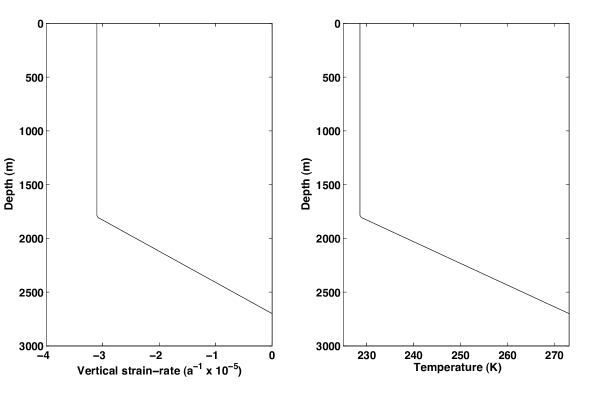
Figure 8: Dansgaard-Johnsen type distributions of the vertical strain rate (left panel) and the temperature at the EDML site (right panel). The depth of the kinks is at two-thirds of the local ice thickness. The strain rate at the surface has been chosen such that the downward vertical velocity equals the accumulation rate, and the surface and basal temperatures match the ice-core data.

According to the topographical data by Wesche et al. [53], the $x$-axis is approximately aligned with the downhill direction, and the gradient of the free surface elevation, $h$, is

$$\frac{\partial h}{\partial x}=-9\times 10^{-4}\pm 10\%,\quad\frac{\partial h}{\partial y}=0.$$ (33)

Thus, in the shallow-ice approximation, the only non-vanishing bed-parallel shear-stress component is $T_{xz}$ ($=S_{xz}$), given by

$$T_{xz}=S_{xz}=\rho gz\frac{\partial h}{\partial x},\qquad$$ (34)

where $g$ is the acceleration due to gravity. Combination with the $x$-$z$-component of the Glen’s flow law (7) yields the isotropic horizontal velocity,

$$v_{x}=-2\rho g\frac{\partial h}{\partial x}\int\limits_{z}^{H}A(T^{\prime})\,\sigma^{n-1}\,\bar{z}\,\mathrm{d}\bar{z}$$ (35)

(e.g., Greve [18], Greve and Blatter [20]), where $H$ is the ice thickness, the rate factor $A(T^{\prime})$ and stress exponent $n$ are chosen as listed in Sect. 2.1, and the enhancement factor $E$ has been set to unity. Similarly, for anisotropic conditions and the corresponding flow law (15), the horizontal velocity is

$$v_{x}=-2\rho g\frac{\partial h}{\partial x}\int\limits_{z}^{H}\hat{E}(\mathcal{A})\,A(T^{\prime})\,\sigma^{n-1}\,\bar{z}\,\mathrm{d}\bar{z},$$ (36)

with the enhancement factor function $\hat{E}(\mathcal{A})$ of Eq. (17). Note that no-slip conditions have been assumed at the ice base, that is, $v_{x}(z\!=\!H)=0$.

The unknowns in Eq. (36) are the normal deviatoric stresses ($S_{xx}$, $S_{yy}$, $S_{zz}$) which are required together with the shallow-ice shear stress (34) for computing the deformability $\mathcal{A}$ by Eq. (14), and then the enhancement factor $\hat{E}(\mathcal{A})$ by Eq. (17). The normal deviatoric stresses are computed by application of the inverse anisotropic flow law (18) with the deformability in the form (23). The latter is evaluated with the calculated shallow-ice deformations and an assumed vertical strain rate $D_{zz}$ in the form of a Dansgaard-Johnsen type distribution [7], which consists of a constant value of $D_{zz}$ from the free surface down to two thirds of the ice thickness, and a linearly decreasing value of $D_{zz}$ below. A similar distribution is employed for the temperature profile (see Fig. 8). We also assume extension in the $x$-direction only, so that the only non-zero horizontal strain rate entering the evaluation of Eq. (23) is $D_{xx}=-D_{zz}$. The vertical velocity $v_{z}$ results from integrating the prescribed vertical strain rate $D_{zz}$, which gives a linear/quadratic profile (e.g., Greve et al. [21]).

For the ODF, we use the preliminary data of the EDML fabric described above. However, since during the drilling process the orientation of the core is not fixed, the horizontal orientation of the non-circularly symmetric girdle fabric (between approximately 600 and 2040 m depth) relative to our coordinate system, i.e., the direction of ice flow, is unknown. For this reason, we need to assign an orientation for the fabric when computing the enhancement factor. We consider two limiting cases by rotating the initial data such that the girdle fabric at all depths is aligned with the $x$-axis (case “R13”) and with the $y$-axis (case “R23”), respectively. This is illustrated in Fig. 3.1.

Figure 9: Sketch of the rotation of the girdle fabrics in order to align with the $x$-axis (case “R13”) and with the $y$-axis (case “R23”) in the Schmidt projection.

At the surface, we assume isotropic conditions, so that $\mathcal{A}_{\mathrm{s}}=1$, and for the maximum softening and hardening parameters, we use the values $E_{\mathrm{max}}=10$ and $E_{\mathrm{min}}=0$, respectively.

In a second step, we attempt at solving the fabric evolution equation (25). For the lack of better knowledge, we neglect recrystallization, that is, we set $\lambda=0$ and $\Gamma=0$ in the constitutive relations (29) and (32), respectively. By allowing only a dependency of the orientation mass density $\rho^{\star}$ on the vertical coordinate $z$ (one-dimensional steady-state problem) and on the orientation $\bf\textstyle n$, the orientation mass balance (25) yields an equation which governs the fabric evolution along the EDML ice core,

$$\frac{\partial\rho^{\star}}{\partial z}v_{z}+\partial_{i}(\rho^{\star}u_{i}^{\star})=0,$$ (37)

where the orientational gradient operator $\partial_{i}$ and the orientation transition rate $u_{i}^{\star}$, respectively, read in index notation as

$$\partial_{i}=\frac{\partial}{\partial n_{i}}-n_{i}n_{j}\frac{\partial}{\partial n_{j}}$$ (38)

and, due to Eq. (28),

$$u^{\star}_{i}=\iota D_{hk}n_{h}n_{k}n_{i}-\iota D_{ij}n_{j}+W_{ij}n_{j}.$$ (39)

With Eq. (38), and by inserting the constitutive relation Eq. (39) in Eq. (37), it follows

$$\begin{array}[b]{l}\mbox{$\displaystyle\frac{\partial\rho^{\star}}{\partial z}$}v_{z}+u_{i}^{\star}\partial_{i}\rho^{\star}+\rho^{\star}\partial_{i}u_{i}^{\star}\\[10.76385pt] =\mbox{$\displaystyle\frac{\partial\rho^{\star}}{\partial z}$}v_{z}+(W_{ij}-\iota D_{ij})n_{j}\partial_{i}\rho^{\star}\\[8.61108pt] \hskip 39.83385pt+\;3\iota\rho^{\star}D_{hk}n_{k}n_{h}=0.\end{array}$$ (40)

We assume that the local flow field consists of vertical compression with the compression rate (negative vertical strain rate) $\varepsilon=-\partial{}v_{z}/\partial{}z$ according to Fig. 8, horizontal extension in $x$-direction, and the horizontal, bed-parallel shear rate

$$\gamma=\frac{\partial v_{x}}{\partial z}=2\rho g\frac{\partial h}{\partial x}\,\hat{E}(\mathcal{A})\,A(T^{\prime})\,\sigma^{n-1}\,z$$ (41)

that results from Eq. (36). The velocity gradient $\mathchoice{\mbox{$\sf\displaystyle L$}}{\mbox{$\sf\textstyle L$}}{\mbox{$\sf\scriptstyle L$}}{\mbox{$\sf\scriptscriptstyle L$}}=\mbox{grad}\,\mathchoice{\mbox{\boldmath$\bf\displaystyle v$}}{\mbox{\boldmath$\bf\textstyle v$}}{\mbox{\boldmath$\bf\scriptstyle v$}}{\mbox{\boldmath$\bf\scriptscriptstyle v$}}$ then reads

$$\mathchoice{\mbox{$\sf\displaystyle L$}}{\mbox{$\sf\textstyle L$}}{\mbox{$\sf\scriptstyle L$}}{\mbox{$\sf\scriptscriptstyle L$}}=\left(\begin{array}[]{ccc}{\varepsilon}&{0}&{\gamma}\\ {0}&{0}&{0}\\ {0}&{0}&{-\varepsilon}\end{array}\right).$$ (42)

Consequently, we obtain for the strain-rate tensor $\sf\textstyle D$ and the spin tensor $\sf\textstyle W$

$$\mathchoice{\mbox{$\sf\displaystyle D$}}{\mbox{$\sf\textstyle D$}}{\mbox{$\sf\scriptstyle D$}}{\mbox{$\sf\scriptscriptstyle D$}}=\left(\begin{array}[]{ccc}{\varepsilon}&{0}&{\mbox{$\frac{1}{2}$}{}\gamma}\\ {0}&{0}&{0}\\ {\mbox{$\frac{1}{2}$}{}\gamma}&{0}&{-\varepsilon}\end{array}\right)$$ (43)

and

$$\mathchoice{\mbox{$\sf\displaystyle W$}}{\mbox{$\sf\textstyle W$}}{\mbox{$\sf\scriptstyle W$}}{\mbox{$\sf\scriptscriptstyle W$}}=\left(\begin{array}[]{ccc}{0}&{0}&{\mbox{$\frac{1}{2}$}{}\gamma}\\ {0}&{0}&{0}\\ {-\mbox{$\frac{1}{2}$}{}\gamma}&{0}&{0}\end{array}\right).$$ (44)

With these expressions and the introduction of spherical coordinates, Eq. (40) reduces to

$$\begin{array}[b]{l}4\mbox{$\displaystyle\frac{\partial\rho^{\star}}{\partial z}$}v_{z}\\[10.76385pt] +\;3\iota\rho^{\star}\big{[}\varepsilon(2\sin^{2}{\theta}\cos{2\varphi}-1-3\cos{2\theta})\\[10.76385pt] \hskip 31.29802pt+\;2\gamma\sin{2\theta}\cos{\varphi}\big{]}\\[8.61108pt] +\;2\mbox{$\displaystyle\frac{\partial\rho^{\star}}{\partial\varphi}$}\Big{[}\varepsilon\iota\sin{2\varphi}+\;\gamma(-1+\iota)\,\mbox{$\displaystyle\frac{\sin{\varphi}}{\tan{\theta}}$}\Big{]}\\[10.76385pt] +\;2\mbox{$\displaystyle\frac{\partial\rho^{\star}}{\partial\theta}$}\Big{[}-\mbox{$\displaystyle\frac{1}{2}$}\iota\varepsilon\sin{2\theta}\,(\cos{2\varphi}+3)\\[10.76385pt] \hskip 41.25648pt+\;\gamma(1-\iota\cos{2\theta})\cos{\varphi}\Big{]}=0,\end{array}$$ (45)

where $\theta$ and $\varphi$ are the polar angle (co-latitude) and azimuth angle (longitude), respectively. Note that, due to Eq. (41), the shear rate $\gamma$ depends on the fabric via the deformability $\mathcal{A}$.

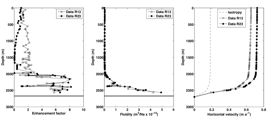
Figure 10: Variation of the enhancement factor (left panel), the ice fluidity (middle panel) and the horizontal velocity (right panel) along the EDML ice core. “Data R13” and “Data R23” represent the solutions obtained with the measured girdle fabrics rotated to align with the $x$- and $y$-direction, respectively, and “Isotropy” represents isotropic conditions.

The shear flow at the EDML station leads to the transport of ice particles over significant horizontal distances. Huybrechts et al. [25] estimate, based on three-dimensional flow modelling, that particles at 89% depth of the core originate from $\approx{}184\,\mathrm{km}$ upstream. This is not taken into account in our spatially one-dimensional model. However, the variation of the shear upstream of the drill site is likely small due to the small variation of the surface gradient (Fig. 3.1), so that the error resulting from the neglected horizontal inhomogeneity should be limited.

In this study, we restrict the solution of Eq. (45) to the simplified case of a transversely isotropic (circularly symmetric) fabric, so that the OMD $\rho^{\star}$ is only a function of the depth $z$ and the polar angle $\theta$. Then Eq. (45) becomes, after integration over the azimuth angle $\varphi$,

$$\begin{array}[b]{l}4\mbox{$\displaystyle\frac{\partial\rho^{\star}}{\partial z}$}v_{z}-\mbox{$\displaystyle\frac{\partial\rho^{\star}}{\partial\theta}$}3\iota\varepsilon\sin{2\theta}\\[10.76385pt] \hskip 34.1433pt-\;3\iota\rho^{\star}\varepsilon(1+3\cos{2\theta})=0.\end{array}$$ (46)

Equation (46) is solved by using a finite-difference discretization with the parameter $\iota=0.6$.

3.2 Results

Figure 10 shows the variation of the enhancement factor, the ice fluidity and the horizontal velocity along the ice core, computed with the ODF based on the fabric data described above. For both limiting cases R13 and R23, the enhancement factor is close to unity in the upper 600 m, which reflects the nearly isotropic fabrics in that part of the EDML core. Further down, in the girdle fabric regime, the case R13 is characterized by a moderate increase of the enhancement factor to an average value of about two, whereas the case R23 exhibits a strong decrease of the enhancement factor to values close to zero. This demonstrates clearly that the girdle fabrics produce a significantly different mechanical response depending on the orientation relative to the ice flow. Case R23 is probably closer to reality, because in the girdle fabric regime above 2000 m depth the deformation is essentially pure shear (vertical compression, horizontal extension in $x$-direction only). For this situation, a simple “deck-of-cards” model illustrates that the $c$-axes turn away from the $x$-axis and towards the $z$-axis, whereas nothing happens in $y$-direction, so that in the Schmidt projection a concentration perpendicular to the $x$-axis (flow direction) results.

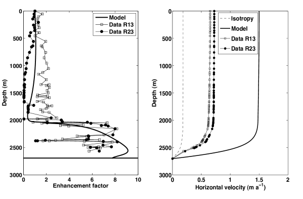
Figure 11: Variation of the enhancement factor (left panel) and the horizontal velocity (right panel) along the EDML ice core. “Model” represents the solutions based on the fabric evolution equation (46) for transverse isotropy. For “Data R13”, “Data R23” and “Isotropy” see the caption of Fig. 10.

Below 2000 m depth, where the fabric switches to a single maximum, the difference between the cases R13 and R23 essentially vanishes. The crystallite basal planes are favourably oriented for the now prevailing simple-shear deformation, which leads to large deformabilities. Consequently, the enhancement factor shows a sharp increase to a maximum value of about eight, which is close to the theoretical maximum of $E_{\mathrm{max}}=10$.

The variabilities of the enhancement factor and the effective stress, as well as the increase of the temperature with depth, contribute to the fluidity profiles shown in Fig. 10b. Since the fluidity is very small above 2000 m depth and increases only further down, the difference between the cases R13 and R23 in absolute values is surprisingly small. At 2563 m depth, the fluidity is about 200 times higher than the fluidity at 1000 m depth for the case R23 due to the counteracting contributions from the favourably oriented $c$-axes, the higher temperature and the smaller effective stress. The latter is somewhat surprising; it is caused by the normal deviatoric stresses $S_{xx}$ and $S_{zz}$, which decrease strongly below 2000 m depth and outweigh the influence of the increasing shear stress $S_{xz}$ in the effective stress.

Owing to the large enhancement factors close to the bottom, the anisotropic flow law predicts significantly larger horizontal velocities compared to the isotropic flow law for the entire depth of the ice core (Fig. 10c). At the surface, the anisotropic horizontal velocities are by approximately a factor 3.5 larger than their isotropic counterparts, and the absolute value of $\approx{}0.7\,\mathrm{m\,a^{-1}}$ agrees very well with measurements (H. Oerter, pers. comm. 2005; Wesche et al. [53]). The difference between the cases R13 and R23 amounts to $\approx{}10\%$, the larger values being obtained for the case R23 owing to the slightly larger enhancement factors below 2000 m depth. Interestingly, these differences show that the fabrics are not perfectly transversely isotropic below 2000 m depth, even though they are very close to the single-maximum type.

Let us now turn to the simulation in which the fabric evolution is computed by solving Eq. (46) for a transversely isotropic fabric. Although this assumption is not consistent with the observed girdle fabric between approximately 600 and 2000 m depth and is therefore a gross simplification, it is interesting to study the mechanical response of such a simplified system and the differences to the ice flow resulting from applying the measured fabrics.

Figure 11a shows the comparison between the enhancement factors resulting from the computed, transversely isotropic fabric (which will be referred to as “modelled enhancement factor” in the following) and from the fabric data. Evidently, the agreement is good despite the assumption of transverse isotropy. Down to 1800 m depth, the modelled enhancement factor lies in between the cases R13 and R23, which are the limiting cases for the orientation of the measured girdle fabric with respect to the ice-flow direction. Between 1800 and 1900 m depth, the modelled enhancement factor is very close to the low values of the case R23, for which the girdle fabric is aligned perpendicular to the flow direction. Below 2000 m depth, the sharp increase is also well reproduced; however, the maximum of the modelled enhancement factor is more pronounced and lies closer to the bottom than for the cases R13 and R23.

For that reason, the modelled enhancement factor leads to larger near-basal shear rates than the enhancement factor based on the cases R13 and R23. Consequently, the horizontal velocity resulting from the modelled enhancement factor is larger by about a factor two than the velocities for the cases R13 and R23 (Fig. 11b). At the surface, a value of $\approx{}1.5\,\mathrm{m\,a^{-1}}$ is reached, which is twice the measured surface velocity. This highlights the great sensitivity of the ice dynamics to the processes near the bottom, which are most difficult to model precisely. Beside the assumption of transverse isotropy, a weak point in that context is the neglection of recrystallization processes, which are expected to become important for the fabric evolution in the lower part of the ice core. This point requires further attention.

4 Conclusions

The newly developed CAFFE model (Continuum-mechanical, Anisotropic Flow model, based on an anisotropic Flow Enhancement factor), which comprises an anisotropic flow law as well as a fabric evolution equation, was presented in this study. It is a good compromise between physical adequateness and simplicity, and is therefore well suited for being used in flow models of ice sheets and glaciers.

The CAFFE model was successfully applied to the site of the EDML ice core in East Antarctica. Two different methods were employed, (i) computing the anisotropic enhancement factor and the horizontal flow based on fabrics data, and (ii) solving the fabric evolution equation under the simplifying assumption of transverse isotropy. Method (i) demonstrated clearly the importance of the anisotropic fabric in the ice column for the flow velocity, and better agreement with the measured surface velocity was achieved compared to an isotropic computation. The anisotropic enhancement factor produced with method (ii) agreed reasonably well with that of method (i), despite the fact that the measured fabric is not transversely isotropic in large parts of the ice core.

A solution of the fabric evolution equation (45) for the EDML ice core without the assumption of transverse isotropy has been presented elsewhere (Seddik et al. [48]). Further, the CAFFE model has already been implemented in the three-dimensional, full-Stokes ice-flow model Elmer/Ice (Seddik [47], Seddik et al. [49]) in order to simulate the ice flow in the vicinity within $100\,\mathrm{km}$ around the Dome Fuji drill site (Motoyama [36]) in central East Antarctica.

References

- [1] N. Azuma. A flow law for anisotropic ice and its application to ice sheets. Earth Planet. Sci. Lett., 128(3-4):601–614, 1994.
- [2] N. Azuma. A flow law for anisotropic polycrystalline ice under uniaxial compressive deformation. Cold Reg. Sci. Technol., 23(2):137–147, 1995.
- [3] W. F. Budd and T. H. Jacka. A review of ice rheology for ice sheet modelling. Cold Reg. Sci. Technol., 16(2):107–144, 1989.
- [4] O. Castelnau, H. Shoji, A. Mangeney, H. Milsch, P. Duval, A. Miyamoto, K. Kawada, and O. Watanabe. Anisotropic behavior of GRIP ices and flow in central Greenland. Earth Planet. Sci. Lett., 154(1-4):307–322, 1998.
- [5] O. Castelnau, T. Thorsteinsson, J. Kipfstuhl, P. Duval, and G. R. Canova. Modelling fabric development along the GRIP ice core, central Greenland. Ann. Glaciol., 23:194–201, 1996.
- [6] Y. F. Dafalias. Orientation distribution function in non-affine rotations. J. Mech. Phys. Solids, 49(11):2493–2516, 2001.
- [7] W. Dansgaard and S. J. Johnsen. A flow model and a time scale for the ice core from Camp Century, Greenland. J. Glaciol., 8(53):215–223, 1969.
- [8] G. Durand, A. Persson, D. Samyn, and A. Svensson. Relation between neighbouring grains in the upper part of the NorthGRIP ice core – implications for rotation recrystallization. Earth Planet. Sci. Lett., 265(3):666–671, 2008.
- [9] S. H. Faria. Mechanics and thermodynamics of mixtures with continuous diversity. Doctoral thesis, Department of Mechanics, Darmstadt University of Technology, Germany, 2003.
- [10] S. H. Faria. Creep and recrystallization of large polycrystalline masses. I. General continuum theory. Proc. R. Soc. A, 462(2069):1493–1514, 2006.
- [11] S. H. Faria. Creep and recrystallization of large polycrystalline masses. III. Continuum theory of ice sheets. Proc. R. Soc. A, 462(2073):2797–2816, 2006.
- [12] S. H. Faria, G. M. Kremer, and K. Hutter. Creep and recrystallization of large polycrystalline masses. II. Constitutive theory for crystalline media with transversely isotropic grains. Proc. R. Soc. A, 462(2070):1699–1720, 2006.
- [13] O. Gagliardini, F. Gillet-Chaulet, and M. Montagnat. A review of anisotropic polar ice models: from crystal to ice-sheet flow models. Low Temp. Sci., 68(Suppl.):149–166, 2009 (this volume).
- [14] F. Gillet-Chaulet, O. Gagliardini, J. Meyssonnier, M. Montagnat, and O. Castelnau. A user-friendly anisotropic flow law for ice-sheet modelling. J. Glaciol., 51(172):3–14, 2005.
- [15] F. Gillet-Chaulet, O. Gagliardini, J. Meyssonnier, T. Zwinger, and J. Ruokolainen. Flow-induced anisotropy in polar ice and related ice-sheet flow modelling. J. Non-Newtonian Fluid Mech., 134:33–43, 2006.
- [16] G. Gödert. A mesoscopic approach for modelling texture evolution of polar ice including recrystallization phenomena. Ann. Glaciol., 37:23–28, 2003.
- [17] G. Gödert and K. Hutter. Induced anisotropy in large ice shields: theory and its homogenization. Cont. Mech. Thermodyn., 10(5):293–318, 1998.
- [18] R. Greve. A continuum-mechanical formulation for shallow polythermal ice sheets. Phil. Trans. R. Soc. Lond. A, 355(1726):921–974, 1997.
- [19] R. Greve. Relation of measured basal temperatures and the spatial distribution of the geothermal heat flux for the Greenland ice sheet. Ann. Glaciol., 42:424–432, 2005.
- [20] R. Greve and H. Blatter. Dynamics of Ice Sheets and Glaciers. Springer, Berlin, Germany etc., 2009.
- [21] R. Greve, Y. Wang, and B. Mügge. Comparison of numerical schemes for the solution of the advective age equation in ice sheets. Ann. Glaciol., 35:487–494, 2002.
- [22] I. Hamann, S. Kipfstuhl, and A. Lambrecht. Ice-fabrics study in the EDML deep ice core (Antarctica). Paper in preparation, 2009.
- [23] R. LeB. Hooke. Principles of Glacier Mechanics. Cambridge University Press, Cambridge, UK and New York, NY, USA, 2nd edition, 2005.
- [24] K. Hutter. Theoretical Glaciology; Material Science of Ice and the Mechanics of Glaciers and Ice Sheets. D. Reidel Publishing Company, Dordrecht, The Netherlands, 1983.
- [25] P. Huybrechts, O. Rybak, F. Pattyn, U. Ruth, and D. Steinhage. Ice thinning, upstream advection, and non-climatic biases for the upper 89% of the EDML ice core from a nested model of the Antarctic ice sheet. Clim. Past, 3(4):577–589, 2007.
- [26] D. Ktitarev, G. Gödert, and K. Hutter. Cellular automaton model for recrystallization, fabric, and texture development in polar ice. J. Geophys. Res., 107(B8):2165, 2002.
- [27] R. Lebensohn, Y. Liu, and P. Ponte Castañeda. Macroscopic properties and field fluctuations in model power-law polycrystals: full-field solutions versus self-consistent estimates. Proc. R. Soc. A, 460:1381–1405, 2004.
- [28] R. Lebensohn, Y. Liu, and P. Ponte Castañeda. On the accuracy of the self-consistent approximation for polycrystals: comparison with full-field numerical simulations. Acta Materialia, 52(18):5347–5361, 2004.
- [29] L. Lliboutry. Anisotropic, transversely isotropic nonlinear viscosity of rock ice and rheological parameters inferred from homogenization. Int. J. Plast., 9:619–632, 1993.
- [30] P. Mansuy, J. Meyssonnier, and A. Philip. Localization of deformation in polycrystalline ice: experiments and numerical simulations with a simple grain model. Comp. Mater. Sci., 25(1-2):142–150, 2002.
- [31] J. Meyssonnier and A. Philip. Comparison of finite-element and homogenization methods for modelling the viscoplastic behaviour of a s2-columnar-ice polycrystal. Ann. Glaciol., 30:115–120, 2000.
- [32] A. Miyamoto. Mechanical properties and crystal textures of Greenland deep ice cores. Doctoral thesis, Hokkaido University, Sapporo, Japan, 1999.
- [33] L. W. Morland. Thermomechanical balances of ice sheet flows. Geophys. Astrophys. Fluid Dyn., 29:237–266, 1984.
- [34] L. W. Morland and R. Staroszczyk. Viscous response of polar ice with evolving fabric. Cont. Mech. Thermodyn., 10(3):135–152, 1998.
- [35] L. W. Morland and R. Staroszczyk. Stress and strain-rate formulations for fabric evolution in polar ice. Cont. Mech. Thermodyn., 15(1):55–71, 2003.
- [36] H. Motoyama. The second deep ice coring project at Dome Fuji, Antarctica. Sci. Drill., 5:41–43, 2007.
- [37] W. S. B. Paterson. Why ice-age ice is sometimes “soft”. Cold Reg. Sci. Technol., 20(1):75–98, 1991.
- [38] W. S. B. Paterson. The Physics of Glaciers. Pergamon Press, Oxford, UK etc., 3rd edition, 1994.
- [39] P. Pimienta, P. Duval, and V. Y. Lipenkov. Mechanical behaviour of anisotropic polar ice. In E. D. Waddington and J. S. Walder, editors, The Physical Basis of Ice Sheet Modelling, IAHS Publication No. 170, pages 57–66. IAHS Press, Wallingford, UK, 1987.
- [40] L. Placidi. Thermodynamically consistent formulation of induced anisotropy in polar ice accounting for grain-rotation, grain-size evolution and recrystallization. Doctoral thesis, Department of Mechanics, Darmstadt University of Technology, Germany, 2004.
- [41] L. Placidi. Microstructured continua treated by the theory of mixtures. Doctoral thesis, University of Rome “La Sapienza”, 2005.
- [42] L. Placidi, R. Greve, H. Seddik, and S. H. Faria. Continuum-mechanical, Anisotropic Flow model for polar ice masses, based on an anisotropic Flow Enhancement factor. Cont. Mech. Thermodyn., 2009. doi: 10.1007/s00161-009-0126-0.
- [43] L. Placidi and K. Hutter. An anisotropic flow law for incompressible polycrystalline materials. Z. angew. Math. Phys., 57:160–181, 2006.
- [44] L. Placidi and K. Hutter. Thermodynamics of polycrystalline materials treated by the theory of mixtures with continuous diversity. Cont. Mech. Thermodyn., 17(6):409–451, 2006.
- [45] D. S. Russell-Head and W. F. Budd. Ice sheet flow properties derived from borehole shear measurements combined with ice core studies. J. Glaciol., 24(90):117–130, 1979.
- [46] F. Saito and A. Abe-Ouchi. Thermal structure of Dome Fuji and east Dronning Maud Land, Antarctica, simulated by a three-dimensional ice-sheet model. Ann. Glaciol., 39:433–438, 2004.
- [47] H. Seddik. A full-Stokes finite-element model for the vicinity of Dome Fuji with flow-induced ice anisotropy and fabric evolution. Doctoral thesis, Graduate School of Environmental Science, Hokkaido University, Sapporo, Japan, 2008.
- [48] H. Seddik, R. Greve, L. Placidi, I. Hamann, and O. Gagliardini. Application of a continuum-mechanical model for the flow of anisotropic polar ice to the EDML core, Antarctica. J. Glaciol., 54(187):631–642, 2008.
- [49] H. Seddik, R. Greve, T. Zwinger, and L. Placidi. A full-Stokes ice flow model for the vicinity of Dome Fuji, Antarctica, with induced anisotropy and fabric evolution. The Cryosphere Discuss., 3(1):1–31, 2009.
- [50] B. Svendsen and K. Hutter. A continuum approach for modelling induced anisotropy in glaciers and ice sheets. Ann. Glaciol., 23:262–269, 1996.
- [51] T. Thorsteinsson. Fabric development with nearest-neighbor interaction and dynamic recrystallization. J. Geophys. Res., 107(B1):2014, 2002.
- [52] C. J. van der Veen. Fundamentals of Glacier Dynamics. A. A. Balkema, Rotterdam, The Netherlands, 1999.
- [53] C. Wesche, O. Eisen, H. Oerter, D. Schulte, and D. Steinhage. Surface topography and ice flow in the vicinity of the EDML deep-drilling site, Antarctica. J. Glaciol., 53(182):442–448, 2007.