Algorithms for regional source localization

Abstract

In this paper we use the MAP criterion to locate a region containing a source. Sensors placed in a field of interest divide the latter into smaller regions and take measurements that are transmitted over noisy wireless channels. We propose implementations of our algorithm that consider complete and limited communication among sensors and seek to choose the most likely hypothesis. Each hypothesis corresponds to the event that a given region contains the source. Corrupted measurements are used to calculate conditional posteriors. We prove that the algorithms asymptotically find the correct region almost surely as long as information is available from three or more sensors. We also study the geometric properties of the model that make it possible in some situations to detect the correct region with a unique sensor. Our simulations confirm that the performance of algorithms with complete and limited information ameliorates with decreasing noise.

I Introduction

I-A Problem description and motivation

Source localization has assumed increasing interest, and has been the subject of study for many researchers. The general setting is that one or multiple sources lie in a bounded region $C$, and a group of $N$ sensors divide $C$ into $N$ smaller connected localization regions $W_{i}$ ,where $i\in\{1,\dots,N\}$. They measure a received signal strength originating at a source $s$, the sensors try to cooperatively identify the region $W_{i}$ containing $s$. We set the problem as a multiple hypothesis decision making problem, where hypothesis $H_{i}$ is true if the source lies in the region $W_{i}$. Maximum a posteriori estimation (MAP) is used as a decision making tool. We implement the estimation technique with an all-to-all and a limited communication algorithm. The setting of the problem and the proposed solution prove to have some geometric characteristics that we derive later in the paper. If properly exploited, these characteristics imply the possibility of regional localization with a unique sensor for certain source positions. We also prove almost sure $(a.s.)$ convergence of both our all-to-all and limited communication algorithms. To the best of our knowledge, none of the algorithms in the literature provide a similar convergence result.

I-B Literature review

In the classical setting, a number of sensors collaborate to locate the exact position of a source. The relation between the position of a source and the received signal strength (RSS) is described in [1, 2, 3]. RSS indirectly provides the distance between the source and a sensor. It is easy to formulate a trivial linear algorithm that permits localization from the measurements at three sensors. However, such a linear algorithm may deliver highly inaccurate estimates of the distances, even when the noise is small [4]. On the other hand, several authors [5, 6] treat localization as a nonconvex optimization problem. Gradient descent algorithms can be used to solve the maximum likelihood estimation problems. Other approaches include approximating the nonlinear nonconvex optimization problem by a linear and convex one and then proposing algorithms for the relaxed problem [7].

Following the gradient, and approximating with a linear convex problem have limitations. The gradient descent can get stuck at local minima far from the correct position, leading to the choice of wrong regions, even in the absence of noise [8]. Authors in [5] use a method of projection onto convex sets. A necessary and sufficient condition for the convergence of this algorithm is that the source lies inside the convex hull of the sensors. The limitations of these methods motivated us to look into regional localization. We note that there are instances where the location of the region containing a source is all that is needed. A more detailed listing of the contributions of this paper is presented below.

I-C Contributions

This paper presents the source localization problem in a setting and formulation that to the best of our knowledge are new. We present algorithms based on all-to-all and limited communication that require only the computation of integrals and therefore present a less computationally exhaustive alternative to the current solutions to the localization problem. We also show that as the noise decreases, regional localization can be accomplished with a unique sensor for certain source positions. We show through an asymptotic analysis that choosing Voronoi partitions as localization regions achieves zero probability of error in the two sensors case. The most important advantage of our formulation is that we are able to demonstrate the convergence of our algorithms. We provide the proof of $a.s.$ convergence of our algorithms, a step that tends to be missing in all of the work presented earlier. Finally, the limited communication algorithm is promising for the localization problems involving multiple sources.

I-D Paper organization

The paper proceeds by a problem formulation and an explanation of our proposed solution in Section II. In Section III we derive some asymptotic geometric properties of the MAP algorithm when applied to our setting. Section IV introduces the implementation of the algorithms. The analytical proof of almost sure $(a.s.)$ convergence of our algorithms is presented in Section V. Section VI shows our simulation results and we conclude in Section VII.

II Problem formulation

Consider a compact connected environment $C\subset\mathbb{R}^{2}$. Suppose there are $N$ disjoint regions $W_{i}$, such that $\cup_{i=1}^{N}W_{i}=C$. Suppose also that there are $N$ sensors placed at $x_{i}\in W_{i}$ and that the source located at an unknown location $s\in C$, transmits a signal whose power undergoes lognormal shadowing described below.

The average power loss for an arbitrary Transmitter-Receiver separation is expressed as a function of distance by using a path loss exponent $\beta>2$. The power loss is proportional to a power of the distance between the transmitter and the receiver. For a thorough description of signal attenuation models over communication channels, we refer the reader to [1, 2, 7]. For reasons to be explained shortly, we work with a slight modification of the traditional model used in the literature. This model for the received power at a sensor $i$ is, $P_{r_{i}}=\frac{Pd_{0}}{d_{0}+\|x_{i}-s\|^{\beta}}$, where $\beta$ indicates the rate at which the power loss increases with distance. $d_{0}$ is a nominal distance chosen such that the received power in the vicinity of the source is almost equal to $P$, the transmitted power at the source. Note that while this model gets rid of the singularity at the source, it converges to the same behavior as the classical model used in communication literature $P_{r_{i}}=\frac{P_{1}}{\|x_{i}-s\|^{\beta}}$, when the distance $\|x_{i}-s\|$ is large. Here $P_{1}$ is the power received at a unit distance from the source. Taking noise into account in our model, the received power satisfies

$$\ln P_{r_{i}}=\ln(Pd_{0})-\ln(d_{0}+\|x_{i}-s\|^{\beta})+n_{i},$$ (1)

where $n_{i}$ are zero mean, independent and identically distributed (i.i.d) white gaussian noise with variance $\sigma^{2}$, each associated with a sensor $i$. The joint probability density function of the $\ln P_{r}=[\ln P_{r_{1}},\dots,\ln P_{r_{N}}]^{T}$, conditioned on the hypothesis that the source is at a point $y\in C$ is given by

$$p(\ln P_{r_{1}},\dots,\ln P_{r_{N}}|y)=\frac{1}{(2\pi\sigma^{2})^{N/2}}\\ \cdot\exp\!\Big{(}{-\frac{\sum_{i=1}^{N}\left(\ln P_{r_{i}}-\ln(\frac{Pd_{0}}{d_{0}+\|x_{i}-y\|^{\beta}})\right)^{2}}{2\sigma^{2}}}\Big{)}.$$ (2)

Solving for the exact position of the source requires solving for $\hat{y}$ that will maximize the likelihood of having the received observation which becomes the problem of solving for,

$$\hat{y}=\arg\min_{y}\sum_{i=1}^{N}\left(\ln P_{r_{i}}-\ln(\frac{Pd_{0}}{d_{0}+||x_{i}-y||^{\beta}})\right)^{2}.$$

This is a nonlinear nonconvex optimization problem. Attempts to solve it or approximate its solution are a topic of great interest. In this paper we look for a regional localization, so the conditioning on the exact position $y$ in (2) is replaced by a regional conditioning. The information exchanged between any two communicating sensors are: the position of the sensors, the localization regions associated with each sensor and the logarithms of the received powers (corrupted with log-normal noise). Sensors can share information as soon as they make a measurement. Alternatively when the noise level in the communication channel is known to be high, it is possible for each sensor to average a set of repeated measurements and transmit the averaged logarithm of the received power. Averaging helps decrease the noise variance, and therefore as we expect and will show later, improves the performance. We start by introducing the case of one noisy measurement per sensor.

II-A Posterior density with a single noisy measurement

Since we do not know where the source is, we make a worst case assumption on the knowledge of its position $s$. Specifically, we assume that the density of $s$ obeys:

$$p(s)=\begin{cases}1/A,&\text{if }s\in C,\\ 0,&\text{otherwise.}\end{cases}$$

Here $A$ is the sum of all the areas $A_{j}$ of $W_{j}$, with $j\in\{1,\dots,N\}$. We need to derive the probability density conditioned on each hypothesis.

Lemma II.1 (Regional conditional density)

Let $z=[\ln P_{r_{1}},\dots,\ln P_{r_{i}}]^{T}$, and note that $P(y\in W_{j})=P(H_{j})=\frac{A_{j}}{A}$, then

$$p(z|y\in W_{j})=\frac{1}{A_{j}}\int_{W_{j}}p(z|y)dy.$$ (3)

Proof.

We compute

$$p(z|y\in W_{j})=\frac{d}{dz}\frac{\operatorname{Prob}(Z\leq z,y\in W_{j})}{P(y\in W_{j})}\\ =A\frac{d}{dz}\frac{\int_{-\infty}^{z}\qquad\int_{W_{j}}p(z|y)p(y)dydz}{A_{j}}\\ =A\frac{d}{dz}\frac{\int_{-\infty}^{z}\qquad\int_{W_{j}}\big{(}p(z|y)/A)dydz}{A_{j}}=\frac{\int_{W_{j}}p(z|y)dy}{A_{j}}.$$

∎

From (2) and (3), we obtain

$$p(\ln P_{r_{1}},\dots,\ln P_{r_{N}}|H_{j})P(H_{j})=\frac{1}{A}\int_{W_{j}}\frac{1}{(2\pi\sigma^{2})^{N/2}}\\ \cdot\exp\!\Big{(}-\frac{\sum_{i=1}^{N}\left(\ln P_{r_{i}}-\ln(\frac{Pd_{0}}{d_{0}+\|x_{i}-y\|^{\beta}})\right)^{2}}{2\sigma^{2}}\Big{)}dy.$$ (4)

Similarly, when measurements from only one sensor are studied.

II-B Posterior density with aggregated noisy measurements

In this setting each sensor is allowed to take $k$ repeated noisy measurements. Noise independence is assumed between sensors and between different samples times for each sensor. Then defining

$$\textbf{P}_{r_{i}}(k)=\sum_{l=1}^{k}\frac{P_{r_{i}}(l)}{k},$$ (5)

the variance of the noise becomes $\sigma^{2}(k)=\frac{\sigma^{2}}{k}$. The regional posterior in then becomes

$$p(\ln\textbf{P}_{r_{i}}(k)|H_{j})P(H_{j})=\frac{1}{A}\int_{W_{j}}\frac{1}{(2\pi\sigma^{2}(k))^{1/2}}\\ \cdot\exp\!\Big{(}-\frac{\left(\ln\textbf{P}_{r_{i}}(k)-\ln(\frac{Pd_{0}}{d_{0}+||x_{i}-y||^{\beta}})\right)^{2}}{2\sigma^{2}(k)}\Big{)}dy,$$

and the joint conditional regional posterior becomes:

$$p(\ln\textbf{P}_{r_{1}}(k),\dots,\ln\textbf{P}_{r_{N}}(k)|H_{i})P(H_{i})=\frac{1}{A}\int_{W_{i}}dy\\ \prod_{j=1}^{N}\frac{1}{(2\pi\sigma^{2}(k))^{1/2}}\exp\!\Big{(}-\frac{\left(\ln\textbf{P}_{r_{j}}(k)-\ln(\frac{Pd_{0}}{d_{0}+||x_{j}-y||^{\beta}})\right)^{2}}{2\sigma^{2}(k)}\Big{)}.$$

Note that, as $k~{}\to~{}\infty$, the noise variance approaches zero, and the probability density approaches a delta function.

Remark II.2

Let $\delta$ be the Dirac delta function. In the infinite measurement case, $\lim_{k\to\infty}\sigma^{2}(k)=0$, and the probability density satisfies

$$p(\ln\textbf{P}_{r_{i}}|y)$$

$$=\lim_{k\rightarrow\infty}\frac{1}{(2\pi\sigma(k)^{2})^{1/2}}\exp\!\Big{(}-\frac{\left(\ln\textbf{P}_{r_{i}}-\ln(\frac{Pd_{0}}{d_{0}+||x_{i}-y||^{\beta}})\right)^{2}}{2\sigma^{2}(k)}\Big{)}$$

$$=\delta\Big{(}\ln\textbf{P}_{r_{i}}-\ln\frac{Pd_{0}}{d_{0}+\|x_{i}-y\|^{\beta}}\Big{)}. \square$$

Remark II.3

In the sequel, for notational simplicity we will treat the aggregated measurement case as if it were identical to the single measurement case with the caveat that the variance goes to zero. $\square$

II-C All-to-all information MAP estimation

In the all-to-all communication (A2A) case, full information is available. Using the conditional probability in (4) MAP selects the hypothesis $H_{i^{*}}$ according to

$$i^{*}=\arg\max_{i}p(\ln P_{r_{1}},\dots,\ln P_{r_{n}}|H_{i})P(H_{i}).$$ (6)

Per Remark II.3, this selection scheme applies to both the single and the aggregated measurement cases.

Before we proceed to deriving the results in the next section, we introduce the definition of the Voronoi diagrams.

Definition II.4 (Voronoi Diagrams)

Given $N$ sensors located at positions $\{x_{1},\dots,x_{N}\}\in C$, we define the Voronoi diagram associated with the $i$th sensor, as follows

$$V_{i}=\{x\in C:\|x-x_{i}\|\leq\|x-x_{j}\|,\forall j\neq i\}.$$

III Preliminary properties of regional localization for one and two sensors

In this section we derive certain geometric properties of MAP estimation as $k~{}\to~{}\infty$ in (5). These geometric properties allow us to conclude the following two results. First, for certain source locations, a single sensor suffices to asymptotically detect the correct hypothesis. Second, for the asymptotic detection problem with two sensors, the selection of Voronoi partitions as localization regions leads to exact localization. These $2$ results should be viewed against the fact that, even in the noise-free case, at least $3$ non-collinear sensors are needed for exact localization. In this section we conduct a large sample analysis to prove an interesting geometric interpretation of the conditional probability densities. This analysis recognizes that when $k~{}\to~{}\infty$ in (5), the Gaussian density approaches a Dirac delta function. Before we state the lemma that captures this property, we mention a basic property of the Dirac delta function [9].

Lemma III.1 (On the Dirac delta function)

If $g:\mathbb{R}\rightarrow\mathbb{R}$ is differentiable and vanishes at positions $x_{\gamma}$, $\gamma\in\Gamma$, then

$$\delta[g(x)]=\sum_{\gamma\in\Gamma}\frac{\delta(x-x_{\gamma})}{|g^{\prime}(x_{\gamma})|}.$$ (7)

In keeping with Remark II.3, consider the situation where

$$p(\ln P_{r_{i}}|y\in W_{j})P(y\in W_{j})\\ =\frac{1}{A}\int_{W_{j}}\delta\left(\ln P_{r_{i}}-\ln\frac{Pd_{0}}{d_{0}+\|x_{i}-y\|^{\beta}}\right)dy.$$

Define the circle $C(r,x_{i})=\{y\in\mathbb{R}^{2}\;|\;\|y-x_{i}\|=r\}$ and denote its intersection with the region $W_{j}$ by $S(W_{j},r,x_{i})~{}=~{}C(r,x_{i})\bigcap W_{j}$. Clearly, this intersection set $S(W_{j},r,x_{i})$ is the union of certain arcs of $C(r,x_{i})$. Define $\theta(W_{j},r,x_{i})$ to be the sum of the angles subtended by these arcs. Call $H_{j}=\left(y\in W_{j}\right)$. If we let $y=[y_{1},y_{2}]^{T}$ and define

$$f(y_{1},y_{2},P_{r_{i}})=\ln P_{r_{i}}-\ln Pd_{0}\\ +\ln(d_{0}+((x_{i_{1}}-y_{1})^{2}+(x_{i_{2}}-y_{2})^{2})^{\beta/2}),$$

then

$$\tiny p(\ln P_{r_{i}}|H_{j})P(H_{j})=\frac{1}{A}\int_{W_{j}}\delta(f(y_{1},y_{2},P_{r_{i}}))dy_{2}dy_{1}.$$

We are now ready for the following lemma.

Lemma III.2 (The arc-length property)

Given a region $W_{j}$, the conditional probability density satisfies

$$p(\ln P_{r_{i}}|y\in W_{j})P(y\in W_{j})\\ =\mathop{\frac{1}{A}\int}_{W_{j}}\delta\Big{(}\ln P_{r_{i}}-\ln\frac{Pd_{0}}{d_{0}+\|x_{i}-y\|^{\beta}}\Big{)}dy_{2}dy_{1},$$

and, if we let $r_{i}=(\frac{P}{P_{r_{i}}}-1)^{\beta}$, then

$$p(\ln P_{r_{i}}|y\in W_{j})P(y\in W_{j})=\frac{d_{0}+r_{i}^{\beta}}{A\beta r_{i}^{\beta-2}}\theta(W_{j},r_{i},x_{i}).$$

The proof of the lemma is provided in the appendix. This lemma can be interpreted as follows. Asymptotically, $P_{r_{i}}$ directly provides the circle of radius $r_{i}$ centered at $x_{i}$ where the sensor is located. $\theta(W_{j},r_{i},x_{i})$ is simply the angle subtended by the intersection of this circle with $W_{j}$. The quantity $p(\ln P_{r_{i}}|y\in W_{j})P(y\in W_{j})$ that is used in MAP is proportional to this angle. We describe further the significance of this result after Lemma III.3. In the following lemma, we show that having Voronoi partitions as well as the MAP estimation algorithm, make the probability of error zero in the two sensors case.

Lemma III.3 (Optimality of Voronoi for $2$ sensors)

Consider two points $x_{1}$ and $x_{2}$ in $C\subset\mathbb{R}^{2}$. Let $V_{1}$ and $V_{2}$ be the Voronoi diagrams associated with $x_{1}$ and $x_{2}$. Take $s\in C$ and let $r_{1}=\|s-x_{1}\|$ and $r_{2}=\|s-x_{2}\|$. Then as $k$ in (5) tends to infinity, MAP localization algorithm finds the region containing $s$, with zero probability of error with only two sensors.

Figure 1: This figure shows two nodes $x_{1}$ and $x_{2}$, with a source $s\in V_{1}$.

Proof.

The proof of this lemma follows the same principle as the proof of Lemma III.2. We point out the differences below. In figure 1, the source $s$ is indicated as one of the two points of intersection of the red and green circle. The posterior becomes $h(y_{1},P_{r_{1}},x_{1},P_{r_{2}},x_{2})=\int_{H(a,W_{j})}\delta\left(f(a,y_{2},P_{r_{1}},x_{1})\right)\cdot\delta\left(f(a,y_{2},P_{r_{2}},x_{2})\right)dy_{2},$ here $P_{r_{1}}$ and $P_{r_{2}}$ are the received powers by the sensors. The integrals are non zero only at the intersections of two sets which we prove to be nothing but the intersection of the circles in Figure 1. The definition of Voronoi (Def. II.4) implies in the two sensors case that if $s^{\prime}\in C$, then $s\in V_{1}\implies s^{\prime}\in V_{1}$. In fact $s\in V_{1}\iff\|x_{1}-s\|\leq\|x_{2}-s\|\iff\|x_{1}-s^{\prime}\|\leq\|x_{2}-s^{\prime}\|\iff s^{\prime}\in V_{1},$ if $s^{\prime}\in C$. The other case to consider is $s^{\prime}\notin C$. In this case $s$ is the unique point of intersection of the circles in $C$. Both ways $h$ is non-zero only in the correct region. ∎

The two lemmas presented in this section have interesting implications. Lemma III.2 implies that, for certain source locations and as the noise becomes smaller, the MAP estimation algorithm can determine the correct region containing the source with only one sensor. That is true when the circle centered at a sensor location with radius $r_{i}$ is included in the region $W_{j}$. Lemma III.3 on the other hand, gives one example where the selection of Voronoi partitions as localization regions makes it possible to locate the source with only two sensors. This would not have been the case with two sensors with general convex regions.

In general, the noise will not be vanishing and the decision needs to be made with a finite number of measurements. We will prove in Section V that the algorithms presented in Section IV below converge almost surely as $k~{}\to~{}\infty$ in (5).

IV Decision making algorithms with all-to-all or limited information

In this section we present two algorithms based on the MAP estimation scheme. The regions can take any shape as long as they are compact. In the limited communication case, sensors can only talk to their neighbors. We assume there is a communication graph that describes the information exchange among robots. We consider two cases: the all-to-all (A2A) communication case and the limited communication case. In the A2A we adopt the complete undirected communication graph. In the limited communication case we make the following degree assumption: each node has at least two neighbors, i.e., each node appears in at least two edges.

IV-A All-to-all communication

In this subsection we present the all-to-all communication algorithm (Algorithm #1), where we apply the classical MAP estimation described in Section II-C on the complete network.   Algorithm #1: All-to-all communication MAP
Network: nodes $\{1,\dots,N\}$ with complete communication graph
State of sensor $i$ is $w_{i}:=\{\ln P_{r_{i}},x_{i},W_{i}\}$
Sensor $i$ executes

1:  For all $j\in\{1,\dots,N\}\setminus\{i\}$

2:       transmit state $w_{i}$ and receive state $w_{j}$

3:       calculate $\theta_{j}:=p(\ln P_{r_{1}},\dots,\ln P_{r_{N}}|H_{j})P(H_{j})$

4:  find $j^{*}:=\arg\max_{j\in\{1,\dots,N\}}\theta_{j}$

5:  Return: decision $j^{*}$

 

Assumption IV.1 (A2A connectivity and noncollinearity)

We assume that the graph is complete. That is all nodes can communicate with each other. We also assume that at least three sensors in the graph are non-collinear.

IV-B Limited communication

In the limited communication algorithm, each sensor acquires data from its neighbors and calculates a joint conditional density (4). Each sensor then applies MAP to choose the most likely hypothesis. In Algorithm #2 each sensor adds the hypothesis of the source being outside its neighborhood, computes the corresponding conditional density and compares it to the densities corresponding to neighboring regions. Let $\mathcal{N}_{i}=\{\{j\in\{1,\dots,N\}\;|\;j\textrm{ is a neighbor of }i\}\operatorname{\cup}\{i\}\}$ and let $N_{i}=|\mathcal{N}_{i}|$ be its cardinality. We described the “source outside neighborhood” hypothesis as hypothesis number $0$ $(H_{0})$. We also define $\ln P_{r_{\mathcal{N}_{i}}}$ to be the vector composed of all measurements $\ln P_{r_{i}}$ where $i\in\mathcal{N}_{i}$. Finally, we mention that given an event $H_{i}=x\in W_{i}$, the complement event is defined by $\overline{H}_{i}=x\in W^{C}_{i}$. Computing the density in the complement of the neighborhood requires only the addition of information about the total region. In fact by applying the total probability theorem, we get that

$$p(\ln P_{r_{j}}|H_{0})P(H_{0})=p(\ln P_{r_{j}}|\overline{\bigcup_{i\in\mathcal{N}_{j}}H_{i}})P(\overline{\bigcup_{i\in\mathcal{N}_{j}}H_{i}})$$

$$=p(\ln P_{r_{j}|y\in C})P(y\in C)-\sum_{i\in\mathcal{N}_{j}}p(\ln P_{r_{j}}|H_{i})P(H_{i})$$

  Algorithm #2: Limited communication MAP
Network: nodes $\{1,\dots,N\}$ with arbitrary communication graph
State of sensor $i$ is $w_{i}:=\{\ln P_{r_{i}},x_{i},W_{i}\}$
Sensor $i$ executes

1:  For all $j\in\mathcal{N}_{i}$

2:       transmit state $w_{i}$ and receive state $w_{j}$

3:       calculate $\theta_{i,j}:=p(\ln P_{r_{\mathcal{N}_{i}}}|H_{j})P(H_{j})$

4:       calculate $\theta_{i,0}=p(\ln P_{r_{\mathcal{N}_{i}}}|\;H_{0})P(H_{0})$

5:  find $j^{*}:=\arg\max_{i\in\mathcal{N}_{i}\operatorname{\cup}\{0\}}\theta_{i,j}$

6:  Return: decision $j^{*}$

 

Assumption IV.2 (Limited conn. and non-collinearity)

We assume that all nodes can communicate to their neighbors. We also assume that at least three sensors are non-collinear in each neighborhood.

V Convergence of algorithms

In this section we prove that the algorithms presented above give the correct decision $w.p.1$ with three or more non-collinear sensors. In keeping with Remark II.3, we examine (4) as $\sigma~{}\to~{}0^{+}$. We start by stating the following result.

Lemma V.1 (Property of non-collinear sensors)

For $d_{0}>0$ and $\beta>0$, given a source $s\in\mathbb{R}^{2}$ and three non-collinear sensors $x_{1}$, $x_{2}$ and $x_{3}\in\mathbb{R}^{2}$, define the function $f:\mathbb{R}^{2}\rightarrow\mathbb{R}$ by $f(z)=\sum_{i=1}^{3}\left(\ln\frac{d_{0}+\|z-x_{i}\|^{\beta}}{d_{0}+\|s-x_{i}\|^{\beta}}\right)^{2}$. The function $f(z)$ vanishes if and only if $z=s$.

Proof.

In fact, it is easy to check that the sum is zero at $z=s$. Uniqueness of this solution is verified by noting that the sum of the square terms is zero only if all the summands are zero. For that to be true one needs to find $z=(x,y)$ such that $((x-x_{i1})^{2}+(y-x_{i2})^{2})^{\beta/2}=((s_{1}-x_{i1})^{2}+(s_{2}-x_{i2})^{2})^{\beta/2}\doteq(r_{i}^{2})^{\beta/2},$ for $i\in\{1,2,3\}$. Expanding and subtracting, we obtain that a necessary and sufficient condition for uniqueness of the solution is that the three points are non-collinear. ∎

In fact given non-collinear $x_{i}$, $i\in\{1,\dots,N\}$ with $N\geq 3$, a compact region $W_{j}$ and a source $s\notin W_{j}$, there always exists

$$D_{j}=\min_{y\in W_{j}}\|s-y\|=\operatorname{dist}(W_{j},s),$$

such that $D_{j}>0$. Also for a compact regions $W_{j}$, there exists $U_{j}>0$ such that

$$U_{j}\geq\max_{y\in W_{j},i\in\{1,\dots,N\}}\left|\ln\frac{d_{0}+\|y-x_{i}\|^{\beta}}{d_{0}+\|s-x_{i}\|^{\beta}}\right|.$$ (8)

Because of the non-collinearity and the fact that $D_{j}>0$, there exists an $L_{j}>0$ such that

$$L_{j}\leq\min_{y\in W_{j}}\sum_{i=1}^{N}\left(\ln\frac{d_{0}+\|y-x_{i}\|^{\beta}}{d_{0}+\|s-x_{i}\|^{\beta}}\right)^{2}.$$ (9)

This follows from the lemma above (i.e., from the fact that the sum has a unique global minimum at $s$). Define

$$\eta_{j}=\sqrt{U_{j}^{2}+\frac{L_{j}}{\alpha N}}-U_{j},$$ (10)

where $\alpha>1$, then we have the following result.

Lemma V.2

Consider $L_{j}$, $U_{j}$ and $\eta_{j}$ as defined in (8), (9) and (10). Suppose the source $s$ is not in region $W_{j}$, and $|n_{i}|\leq\eta_{j}$ for all $i\in\{1,\dots,N\}$. Then

$$\frac{\alpha-1}{\alpha}L_{j}\leq\min_{y\in W_{j}}\sum_{i=1}^{N}\left(\ln\frac{d_{0}+\|y-x_{i}\|^{\beta}}{d_{0}+\|s-x_{i}\|^{\beta}}+n_{i}\right)^{2}.$$ (11)

Proof.

In fact, the sum in (11) satisfies:

$$\sum_{i=1}^{N} \Big{(}\ln\frac{d_{0}+\|y-x_{i}\|^{\beta}}{d_{0}+\|s-x_{i}\|^{\beta}}+n_{i}\Big{)}^{2}$$

$$\geq L_{j}-2U_{j}N\eta_{j}-N\eta_{j}^{2}=L_{j}+2U_{j}^{2}N$$

$$\quad-2U_{j}N\sqrt{U_{j}^{2}+\frac{L_{j}}{\alpha N}}-N(U_{j}^{2}+\frac{L_{j}}{\alpha N})-NU_{j}^{2}$$

$$\quad+2NU_{j}\sqrt{U_{j}^{2}+\frac{L_{j}}{\alpha N}}=\frac{\alpha-1}{\alpha}L_{j}.$$

∎

For simplicity of notation, we choose $\alpha=2$ from here on. Next, we introduce the final intermediate lemma before the main results of this section.

Lemma V.3 (Upper bound for wrong hypothesis)

Given $L_{j}$, $U_{j}$ and $\eta_{j}$ as defined in (8), (9) and (10), define

$$I_{j}=p(\ln P_{r_{1}},\dots,\ln P_{r_{N}}|H_{j})P(H_{j})=\frac{1}{A(2\pi\sigma^{2})^{N/2}}\\ \cdot\int_{W_{j}}\exp\!\Big{(}-\frac{\sum_{i=1}^{N}\left(\ln P_{r_{i}}-\ln\frac{Pd_{0}}{d_{0}+\|y-x_{i}\|^{\beta}}\right)^{2}}{2\sigma^{2}}\Big{)}dy.$$

If $|n_{i}|\leq\eta_{j}$ for $i\in\{1,\dots,N\}$, then for $j\in\{1,\dots,N\}$

$$I_{j}\leq\frac{A_{j}\exp\!\big{(}-L_{j}/4\sigma^{2}\big{)}}{A(2\pi\sigma^{2})^{N/2}}.$$

Proof.

Because of the equality

$$\ln P_{r_{i}}-\ln\frac{Pd_{0}}{d_{0}+\|y-x_{i}\|^{\beta}}=\ln\frac{d_{0}+\|y-x_{i}\|^{\beta}}{d_{0}+\|s-x_{i}\|^{\beta}}+n_{i},$$

the result directly follows from Lemma V.2 and from the fact that the surface integral of a function $f$ is upper bounded by the surface integral of a constant function $g$, where $g$ takes the maximum value of $f$. ∎

We are now ready for the convergence theorem. As usual, we define the $Q$-function $Q:\mathbb{R}\rightarrow\mathbb{R}_{>0}$ by

$$Q(x)=\frac{1}{\sqrt{2\pi}}\int_{x}^{+\infty}\exp(-y^{2}/2)dy.$$

Theorem V.4 (Elimination property of wrong hypothesis)

Consider $x_{i}$ non-collinear sensors, $i\in\{1,\dots,N\}$ with $N\geq 3$. Let $\sigma$ be the noise variance. Given a source $s\notin W_{j}$, then we have

$$\operatorname{Prob}\biggl{[}p(\ln P_{r_{1}},\dots,\ln P_{r_{N}}|H_{j})P(H_{j})\leq\epsilon_{j}(\sigma)\biggr{]}\geq\mu_{j}(\sigma),$$

where

$$\epsilon_{j}(\sigma)=\frac{A_{j}\exp(-L_{j}/4\sigma^{2})}{A(2\pi\sigma^{2})^{N/2}},\quad\mu_{j}(\sigma)=(1-2Q(\eta_{j}/\sigma))^{N}.$$

Furthermore, as $\sigma\to 0^{+}$, we have $\epsilon_{j}(\sigma)~{}\to~{}0^{+}\quad\text{and}\quad\mu_{j}(\sigma)~{}\to~{}1^{-}$.

Proof.

From Lemmas V.2 and V.3 , we have that

$$\operatorname{Prob} \big{[}p(\ln P_{r_{1}},\dots,\ln P_{r_{N}}|H_{j})P(H_{j})\leq\epsilon_{j}(\sigma)\big{]}$$

$$\geq\operatorname{Prob}\left[[n_{1},\dots,n_{N}]^{T}\in[-\eta_{j},\eta_{j}]^{N}\right]$$

$$=\prod_{i=1}^{N}\biggl{(}\frac{1}{2}-\operatorname{Prob}[n_{i}>\eta_{j}]+\frac{1}{2}-\operatorname{Prob}[n_{i}<-\eta_{j}]\biggr{)}$$

$$=\big{(}1-2Q(\eta_{j}/\sigma)\big{)}^{N}.$$

The first inequality comes from the fact that Lemmas V.2 and V.3 hold whenever all $|n_{i}|\leq\eta_{j}$. The proofs of the two limits of $\epsilon_{j}$ and $\mu_{j}$ are immediate. ∎

This theorem states that, as $\sigma~{}\to~{}0^{+}$, the probability that the joint density function $p(\ln P_{r_{1}},\dots,\ln P_{r_{N}}|H_{j})P(H_{j})$ takes an arbitrarily small value goes arbitrarily close to $1$ when $H_{j}$ is not the correct hypothesis. This is so as $Q(x)~{}\to~{}0$ as $x~{}\to~{}\infty$. To complement the Theorem V.4, we prove below that for the correct hypothesis, the probability density will be lower bounded by a positive term $w.p.1$.

Theorem V.5 (Strict positivity for correct hypothesis)

Consider $x_{i}$ non-collinear sensors, $i\in\{1,\dots,N\}$ with $N\geq 3$. Let $\sigma$ be the noise variance. If $s\in W_{i}$, then we have

$$\operatorname{Prob}\left[p(\ln P_{r_{1}},\dots,\ln P_{r_{N}}|H_{i})P(H_{i})\geq\Psi(\sigma)\right]\geq\Omega(\sigma),$$

where

$$\Psi(\sigma)=p(\ln P_{r_{1}},\dots,\ln P_{r_{N}})-\sum_{\begin{subarray}{c}{j=1,\dots,N}\\ {j\neq i}\end{subarray}}\frac{A_{j}\exp(-L_{j}/4\sigma^{2})}{A(2\pi\sigma^{2})^{N/2}},$$

$$\Omega(\sigma)=\prod_{\begin{subarray}{c}{j=1,\dots,N}\\ {j\neq i}\end{subarray}}\mu_{j}(\sigma)=\prod_{\begin{subarray}{c}{j=1,\dots,N}\\ {j\neq i}\end{subarray}}(1-2Q(\eta_{j}/\sigma))^{N}.$$

Furthermore, as $\sigma~{}\to~{}0^{+}$, we have $\Psi(\sigma)~{}\to~{}p(\ln P_{r_{1}},\dots,\ln P_{r_{N}})>0\quad\text{and}\quad\Omega(\sigma)~{}\to~{}1^{-}$.

Proof.

The proof of this theorem follows directly from Theorem V.4 and the total probability theorem. Call $~{}z=~{}[\ln P_{r_{1}},\dots,\ln P_{r_{N}}]^{T}$. We know from the total probability theorem that

$$p(z) =\sum_{j=1}^{N}p(z|H_{j})P(H_{j})$$

$$=p(z|H_{i})P(H_{i})+\sum_{\begin{subarray}{c}{j=1,\dots,N}\\ {j\neq i}\end{subarray}}p(z|H_{j})P(H_{j})$$

and, in turn, that

$$p(z|H_{i})P(H_{i})=p(z)-\sum_{\begin{subarray}{c}{j=1,\dots,N}\\ {j\neq i}\end{subarray}}p(z|H_{j})P(H_{j}).$$

From Theorem V.4

$$\operatorname{Prob}\left[p(z|H_{i})P(H_{i})\geq p(z)-\sum_{\begin{subarray}{c}{j=1,\dots,N}\\ {j\neq i}\end{subarray}}\epsilon_{j}(\sigma)\right]$$

$$\geq\prod_{\begin{subarray}{c}{j=1,\dots,N}\\ {j\neq i}\end{subarray}}\operatorname{Prob}\biggl{[}p(z|H_{j})P(H_{j})\leq\epsilon_{j}(\sigma)\biggr{]}\geq\prod_{\begin{subarray}{c}{j=1,\dots,N}\\ {j\neq i}\end{subarray}}\mu_{j}(\sigma)$$

As $\sigma~{}\to~{}0^{+}$, $\Psi(\sigma)~{}\to~{}p(z)$ and $\Omega(\sigma)~{}\to~{}1^{-}$. ∎

Theorem V.5 complements Theorem V.4 in that is shows that as $\sigma~{}\to~{}0^{+}$, the probability density conditioned on the correct hypothesis is lower bounded by a strictly positive term. This event happens asymptotically with probability $1$.

Under Assumption IV.1, as MAP follows (6), Theorems V.5 and V.4 complete the proof of $a.s$ convergence of the all-to-all communication MAP algorithm. Similarly for the limited communication, under Assumption IV.2, MAP estimation converges almost surely when applied to regional localization.

VI Simulations

In this section we show simulation results illustrating the type of decision obtained by our algorithms. We also show a comparison plot between the all-to-all and the limited information algorithms.

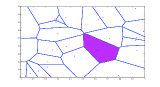
Figure 2: This figure shows the all-to-all communication algorithm with 25 sensors and one source whose region was correctly detected.

The plot in Figure 2 shows a correct detection of the source. The shaded region corresponds to the one detected by the algorithm, the source is shown as a star and the sensors as the dots.

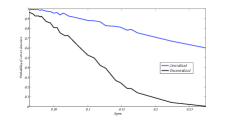
Figure 3: This figure shows the probability of correct decision making of the all-to-all and limited communication cases over $1000$ runs, with $20$ sensors. The blue curve corresponds to the A2A communication algorithm, and the black curve corresponds to the limited communication algorithm (with the majority vote).

Figure 3 shows the results obtained from batches of $1000$ runs, with $N=20$ sensors. The plots are obtained as follows: If $d_{j}$ is the index of the region chosen by sensor $j$, we compare it to the correct index $d^{*}$. For the comparison to be fair, and since the limited communication algorithm makes decisions only about its neighborhood, we compare the two algorithms by adding a communication round to the limited communication algorithm, where we look at all the sensors that decided that the source is in their neighborhood, noting that the decisions could be inconsistent, we run a majority vote among the aforementioned sensors, and compare the final decision to the correct one. The black curve in Figure 3 represents the limited communication decisions, while the blue curve represents the all-to-all communication decision. Figure 3 shows the probability of making a correct decision as $\sigma$ increases. It is not surprising that as the noise variance increases the probability of correct decision making decreases.

VII Conclusion

In this paper we have presented an all-to-all and a limited communication algorithm based on MAP that succeed in identifying a region that contains a source. We have also presented an asymptotic analysis and derived some geometric properties of our algorithms. Those properties had the implication that for certain source positions, it is possible to solve the regional localization problem with a unique sensor. We showed that choosing Voronoi partitions for localization regions asymptotically achieves zero probability of error in the two sensors case. We were also able to prove that when readings from three or more non-collinear sensors are available, the algorithms choose the correct region almost surely. As an extension to this work we are studying how to optimally position the sensors, and choose the localization regions, so that we minimize the probability of error of our algorithms.

Proof of Lemma III.2.

Let

$$H(a,W_{j})=\left(y_{2}\in\mathbb{R}\textrm{ such that given }y_{1}=a,[a,y_{2}]\in W_{j}\right)$$

$$h(y_{1},P_{r_{i}},x_{i})=\\ \int_{H(a,W_{j})}\delta\left(\ln P_{r_{i}}-\ln\frac{Pd_{0}}{d_{0}+\|x_{i}-y\|^{\beta}}\right)dy_{2}\\ =\int_{H(a,W_{j})}\delta\left(f(a,y_{2},P_{r_{i}},x_{i})\right)dy_{2}.$$ (12)

Since

$$\frac{d}{dy_{2}}f(y_{1},y_{2},P_{r_{i}},x_{i})=f^{\prime}(y_{1},y_{2},P_{r_{i}},x_{i})\\ =\frac{\beta}{2}\cdot 2\cdot(-1)\cdot(x_{i_{2}}-y_{2})\frac{\left((x_{i_{1}}-y_{1})^{2}+(x_{i_{2}}-y_{2})^{2}\right)^{\frac{\beta}{2}-1}}{d_{0}+\left((x_{i_{1}}-y_{1})^{2}+(x_{i_{2}}-y_{2})^{2}\right)^{\frac{\beta}{2}}}$$

If we fix $y_{1}=a$, we can solve for $y_{2}(a)$ such that, $f(a,y_{2}(a),P_{r_{i}},x_{i})=0$. In fact

$$f(a,y_{2}(a),P_{r_{i}},x_{i})=0\\ \Leftrightarrow\ln P_{r_{i}}-\ln\frac{Pd_{0}}{d_{0}+\left((x_{i_{1}}-a)^{2}+(x_{i_{2}}-y_{2}(a))^{2}\right)^{\frac{\beta}{2}}}=0\\ \Leftrightarrow(x_{i_{1}}-a)^{2}+(x_{i_{2}}-y_{2}(a))^{2}=\left(\frac{P-P_{r_{i}}}{P_{r_{i}}}d_{0}\right)^{\frac{2}{\beta}}=r_{i}^{2},$$ (13)

where $r_{i}=\left((\frac{P}{P_{r_{i}}}-1)d_{0}\right)^{\frac{1}{\beta}}$. Observe $H(a,W_{j})$ has at most two elements satisfying equation (13), one or both of:

$$y_{2,1}(a)=x_{i_{2}}-\sqrt{r_{i}^{2}-(x_{i_{1}}-a)^{2}}$$ (14)

or,

$$y_{2,2}(a)=x_{i_{2}}+\sqrt{r_{i}^{2}-(x_{i_{1}}-a)^{2}},$$ (15)

whenever $r_{i}^{2}\geq(x_{i_{1}}-a)^{2}$. Using property (7) of the dirac delta function, and substituting with $y_{2,1}(a)$ and $y_{2,2}(a)$ obtained in (14) and (15), (12) becomes:

$$h(a,P_{r_{i}},x_{i})=\int_{H(a,j)}\delta(f(a,y_{2},P_{r_{i}}),x_{i})dy_{2},$$

takes the values

$$\left\{\begin{array}[]{ll}\int_{H(a,W_{j})}\frac{\delta(y_{2}-y_{21}(a))}{|f^{\prime}(a,y_{2},P_{r_{i}},x_{i})|}dy_{2}\\ \textrm{if $y_{2,1}(a)\in H(a,W_{j})$ but $y_{2,2}(a)\notin H(a,W_{j})$}\\ \int_{H(a,W_{j})}\frac{\delta(y-y_{2,2}(a))}{|f^{\prime}(a,y_{2},P_{r_{i}},x_{i})|}\ dy_{2}\\ \textrm{if $y_{2,2}(a)\in H(a,W_{j})$ but $y_{21}(a)\notin H(a,W_{j})$}\\ \int_{H(a,W_{j})}\frac{\delta(y_{2}-y_{2,1}(a))}{|f^{\prime}(a,y_{2},P_{r_{i}},x_{i})|}+\frac{\delta(y_{2}-y_{2,2}(a))}{|f^{\prime}(a,y_{2},P_{r_{i}},x_{i})|}\ dy_{2}\\ \textrm{if both $y_{2,1}(a)$ and $y_{2,2}(a)\in H(a,W_{j})$}\end{array}\right.$$

Define $I_{1}(a,W_{j})$, the indicator function satisfying

$$I_{1}(a,W_{j})=\left\{\begin{array}[]{ll}1&\textrm{if $y_{2,1}(a)\in H(a,W_{j})$}\\ 0&\textrm{otherwise}\end{array}\right.$$

Similarly define $I_{2}(a,W_{j})$, the indicator function satisfying

$$I_{2}(a,W_{j})=\left\{\begin{array}[]{ll}1&\textrm{if $y_{2,2}(a)\in H(a,W_{j})$}\\ 0&\textrm{otherwise}\end{array}\right.$$

Then, (12) becomes

$$h(a,P_{r_{i}},x_{i})=\frac{1}{|f^{\prime}(a,y_{2,1}(a),P_{r_{i}},x_{i})|}I_{1}(a,W_{j})\\ +\frac{1}{|f^{\prime}(a,y_{2,2}(a),P_{r_{i}},x_{i})|}I_{2}(a,W_{j}).$$

By substituting from (14), we get

$$\frac{1}{|f^{\prime}(a,y_{2}(a),P_{r_{i}},x_{i})|}$$

$$= \frac{d_{0}+\left((x_{i_{1}}-a)^{2}+r_{i}^{2}-(x_{i_{1}}-a)^{2}\right)^{\frac{\beta}{2}}}{\beta\sqrt{r_{i}^{2}-(x_{i_{1}}-a)^{2}}\left((x_{i_{1}}-a)^{2}+r_{i}^{2}-(x_{i_{1}}-a)^{2}\right)^{\frac{\beta}{2}-1}}$$

$$= \frac{d_{0}+r_{i}^{\beta}}{\beta\sqrt{r_{i}^{2}-(x_{i_{1}}-a)^{2}}}\frac{1}{r_{i}^{\beta-2}}=\frac{d_{0}+r_{i}^{\beta}}{\beta r_{i}^{\beta-2}}\cdot\frac{1}{\sqrt{r_{i}^{2}-(x_{i_{1}}-a)^{2}}}$$

Let $\mathcal{C}_{j}=\{x\in\mathbb{R}\textrm{ such that }(x,y_{2,1}(x))\in W_{j}\}$ and $\mathcal{C^{\prime}}_{j}=\{x\in\mathbb{R}\textrm{ such that }(x,y_{2,2}(x))\in W_{j}\}$. Note that

$$x\in\mathcal{C}_{j}\Rightarrow I_{1}(x,W_{j})=1\textrm{ and }x\in\mathcal{C^{\prime}}_{j}\Rightarrow I_{2}(x,W_{j})=1.$$

Then,

$$\tiny p (\ln P_{r_{i}}|y\in W_{j})P(y\in W_{j})=\frac{1}{A}\int_{\mathcal{C}_{j}\bigcup\mathcal{C^{\prime}}_{j}}h(y_{1},P_{r_{i}},x_{i})dy_{1}$$

$$=\frac{1}{A}\biggr{(}\int_{\mathcal{C}_{j}}h(y_{1},P_{r_{i}},x_{i})dy_{1}+\int_{\mathcal{C^{\prime}}_{j}}h(y_{1},P_{r_{i}},x_{i})dy_{1}\biggl{)}$$

$$=\frac{1}{A}\int_{\mathcal{C}_{j}}\frac{1}{|f^{\prime}(y_{1},y_{2,1}(y_{1}),P_{r_{i}},x_{i})|}dy_{1}$$

$$+\frac{1}{A}\int_{\mathcal{C^{\prime}}_{j}}\frac{1}{|f^{\prime}(y_{1},y_{2,2}(y_{1}),P_{r_{i}},x_{i})|}dy_{1}.$$ (16)

Write

$$\mathcal{C}_{j}=\bigcup_{\alpha=1}^{s}A_{\alpha}\textrm{ , with }\bigcap_{\alpha}A_{\alpha}=\emptyset\textrm{ , and }A_{\alpha}=[a_{1_{\alpha}},a_{2_{\alpha}}],$$ (17)

$$\mathcal{C^{\prime}}_{j}=\bigcup_{\alpha=1}^{s^{\prime}}A^{\prime}_{\alpha}\textrm{ , with }\bigcap_{\alpha}A^{\prime}_{\alpha}=\emptyset\textrm{ , and }A^{\prime}_{\alpha}=[a^{\prime}_{1_{\alpha}},a^{\prime}_{2_{\alpha}}].$$ (18)

Equation (Proof of Lemma III.2.) can then be written as the sum

$$A\cdot p(\ln P_{r_{i}}|y\in W_{j})P(y\in W_{j})=$$

$$\sum_{\alpha=1}^{s}\int_{A_{\alpha}}\frac{1}{|f^{\prime}(y_{1},y_{2,1}(y_{1}),P_{r_{i}},x_{i})|}dy_{1}$$

$$+\sum_{\alpha=1}^{s^{\prime}}\int_{A^{\prime}_{\alpha}}\frac{1}{|f^{\prime}(y_{1},y_{2,2}(y_{1}),P_{r_{i}},x_{i})|}y_{1}.$$

$$\tiny=\sum_{\alpha=1}^{s}\int_{a_{2_{\alpha}}}^{a_{1_{\alpha}}}\frac{1}{|f^{\prime}(y_{1},y_{2,1}(y_{1}),P_{r_{i}},x_{i})|}dy_{1}\\ +\sum_{\alpha=1}^{s^{\prime}}\int_{a^{\prime}_{1_{\alpha}}}^{a^{\prime}_{2_{\alpha}}}\frac{1}{|f^{\prime}(y_{1},y_{2,2}(y_{1}),P_{r_{i}},x_{i})|}\ dy_{1},$$

$$\tiny=\sum_{\alpha=1}^{s}\int_{a_{2_{\alpha}}}^{a_{1_{\alpha}}}\frac{d_{0}+r_{i}^{\beta}}{\beta r_{i}^{\beta-2}}\cdot\frac{1}{\sqrt{r_{i}^{2}-(x_{i_{1}}-y_{1})^{2}}}\ dy_{1}\\ +\sum_{\alpha=1}^{s^{\prime}}\int_{a^{\prime}_{2_{\alpha}}}^{a^{\prime}_{1_{\alpha}}}\frac{d_{0}+r_{i}^{\beta}}{\beta r_{i}^{\beta-2}}\cdot\frac{1}{\sqrt{r_{i}^{2}-(x_{i_{1}}-y_{1})^{2}}}\ dy_{1}\\ =\sum_{\alpha=1}^{s}\frac{d_{0}+r_{i}^{\beta}}{\beta r_{i}^{\beta-2}}\cdot\arctan\frac{x_{i_{1}}-a}{\sqrt{r_{i}^{2}-(x_{i_{1}}-y_{1})^{2}}}|_{a_{1_{\alpha}}}^{a_{2_{\alpha}}}\\ +\sum_{\alpha=1}^{s^{\prime}}\frac{d_{0}+r_{i}^{\beta}}{\beta r_{i}^{\beta-2}}\cdot\arctan\frac{x_{i_{1}}-y_{1}}{\sqrt{r_{i}^{2}-(x_{i_{1}}-y_{1})^{2}}}|_{a^{\prime}_{1_{\alpha}}}^{a^{\prime}_{2_{\alpha}}}$$

Note that

$$\tiny\arctan\frac{x_{i_{1}}-a}{\sqrt{r_{i}^{2}-(x_{i_{1}}-a)^{2}}}\\ =\arctan\frac{x_{i_{1}}-a}{\sqrt{(x_{i_{1}}-a)^{2}+(x_{i_{2}}-y_{2}(a))^{2}-(x_{i_{1}}-a)^{2}}}\\ =\arctan\frac{x_{i_{1}}-a}{x_{i_{2}}-y_{2}(a)}=\frac{\pi}{2}-\arctan\frac{x_{i_{2}}-y_{2}(a)}{x_{i_{1}}-a}.$$

The conditional probability density becomes after simplifications,

$$\tiny p(\ln P_{r_{i}}|y\in W_{j})P(y\in W_{j})=\frac{d_{0}+r_{i}^{\beta}}{A\beta r^{\beta-2}}\cdot\sum_{\alpha=1}^{s}\\ \left(\frac{\pi}{2}-\arctan\frac{x_{i_{2}}-y_{2}(a_{2_{\alpha}})}{x_{i_{1}}-a_{2_{\alpha}}}-\frac{\pi}{2}+\arctan\frac{x_{i_{2}}-y_{2}(a_{1_{\alpha}})}{x_{i_{1}}-a_{1_{\alpha}}}\right)\\ +\frac{d_{0}+r_{i}^{\beta}}{A\beta r_{i}^{\beta-2}}\sum_{\alpha=1}^{s^{\prime}}\left(\frac{\pi}{2}-\arctan\frac{x_{i_{2}}-y_{2}(a^{\prime}_{2_{\alpha}})}{x_{i_{1}}-a^{\prime}_{2_{\alpha}}}-\frac{\pi}{2}\right.\\ \left.+\arctan\frac{x_{i_{2}}-y_{2}(a^{\prime}_{1_{\alpha}})}{x_{i_{1}}-a^{\prime}_{1_{\alpha}}}\right)=\frac{d_{0}+r_{i}^{\beta}}{A\beta r_{i}^{\beta-2}}\left(\sum_{\alpha=1}^{s}\theta_{\alpha}+\sum_{\alpha=1}^{s^{\prime}}\theta^{\prime}_{\alpha}\right),$$

where $\theta_{\alpha}$ and $\theta^{\prime}_{\alpha}$ are the angles of the arcs in $S(W_{j},r_{i},x_{i})$ described on distinct supports as in (17) and (18) when applicable. ∎

References

• [1] T.Β S. Rappoport, Wireless Communications: Principles and Practice. New Jersey: Prentice Hall, 1996.
• [2] J.Β Proakis and M.Β Salehi, Communication Systems Engineering. Prentice Hall, 2001.
• [3] A.Β Sayed, A.Β Tarighat, and Khajehnouri, β€œNetwork-based wireless location: challenges faced in developping techniques for accurate wireless location information,” IEEE Signal Processing Magazine, vol.Β 22, no.Β 4, 2005.
• [4] M.Β Cao, B.Β Anderson, and A.Β Morse, β€œSensor network localization with imprecise distance measurements,” Systems & Control Letters, vol.Β 55, no.Β 11, 2006.
• [5] A.Β Hero and D.Β Blatt, β€œSensor network source localization via projection onto convex sets (pcos),” in IEEE International Conference on Acoustics, Speech and Signal Processing, pp.Β 689–692, 2005.
• [6] M.Β G. Rabbat and R.Β D. Nowak, β€œDecentralized source localization and trackings,” in IEEE International Conference on Acoustics, Speech and Signal Processing, pp.Β 921–924, 2004.
• [7] C.Β Meng, Z.Β Ding, and S.Β Dasgupta, β€œA semidefinite programming approach to source localization in wireless network,” IEEE Signal Processing Letters, vol.Β 15, pp.Β 389–404, 2008.
• [8] G.Β Mao, B.Β Fidan, and B.Β Anderson, β€œWireless sensor network localization techniques,” Computer Network, vol.Β 51, no.Β 10, pp.Β 2529–2553, 2007.
• [9] K.Β Hecht, Quantum Mechanics. USA: Springer, 1996.
Proof of LemmaΒ III.2.
Let