Joint Bayesian endmember extraction and linear unmixing for hyperspectral imagery

Abstract

This paper studies a fully Bayesian algorithm for endmember extraction and abundance estimation for hyperspectral imagery. Each pixel of the hyperspectral image is decomposed as a linear combination of pure endmember spectra following the linear mixing model. The estimation of the unknown endmember spectra is conducted in a unified manner by generating the posterior distribution of abundances and endmember parameters under a hierarchical Bayesian model. This model assumes conjugate prior distributions for these parameters, accounts for non-negativity and full-additivity constraints, and exploits the fact that the endmember proportions lie on a lower dimensional simplex. A Gibbs sampler is proposed to overcome the complexity of evaluating the resulting posterior distribution. This sampler generates samples distributed according to the posterior distribution and estimates the unknown parameters using these generated samples. The accuracy of the joint Bayesian estimator is illustrated by simulations conducted on synthetic and real AVIRIS images.

I Introduction

Over the last several decades, much research has been devoted to the spectral unmixing problem. Spectral unmixing is an efficient way to solve standard problems encountered in hyperspectral imagery. These problems include pixel classification [1], material quantification [2] and subpixel detection [3]. Spectral unmixing consists of decomposing a pixel spectrum into a collection of material spectra, usually referred to as endmembers, and estimating the corresponding proportions or abundances [4]. To describe the mixture, the most frequently encountered model is the macroscopic model which gives a good approximation in the reflective spectral domain ranging from $0.4\mu$m to $2.5\mu$m [5]. The linearization of the non-linear intimate model proposed by Hapke in [6] results in this macroscopic model [7]. The macroscopic model assumes that the observed pixel spectrum is a weighted linear combination of the endmember spectra.

As reported in [4], linear spectral mixture analysis (LSMA) has often been handled as a two step procedure: the endmember extraction step and the inversion step, respectively. In the first step of analysis, the macroscopic materials that are present in the observed scene are identified by using an Endmember Extraction Algorithm (EEA). The most popular EEAs include PPI [8] and N-FINDR [9], that apply a linear model for the observations with non-negativity and full-additivity constraints. This model results in endmember spectra located on the vertices of a lower dimensional simplex. PPI and N-FINDR estimate this simplex by identifying the largest simplex contained in the data. Another popular alternative, called Vertex Component Analysis (VCA) has been proposed in [10]. A common assumption in VCA, PPI and N-FINDR is that they require pure pixels to be present in the observed scene, where pure pixels are pixels composed of a single endmember. Alternatively, Craig has proposed the Minimum Volume Transform (MVT) to find the smallest simplex that contains all the pixels [11]. However, MVT-based methods (e.g. ORASIS [12]) are not fully automated techniques: they provide results that strongly depend on i) the algorithm initialization, ii) some ad hoc parameters that have to be selected by the user. More generally, these previous EEAs avoid the difficult problem of direct parameter estimation on the simplex. The interested reader is invited to consult [13] and [14] for a recent performance comparison of some standard EEAs.

The second step in LSMA, called the inversion step, consists of estimating the proportions of the materials identified by EEA [15]. The inversion step can use various strategies such as least square estimation [16], maximum likelihood estimation [17] and Bayesian estimation [18].

The central premise of this paper is to propose an algorithm that estimates the endmember spectra and their respective abundances jointly in a single step. This approach casts LSMA as a blind source separation (BSS) problem [19]. In numerous fields, independent component analysis (ICA) [20] has been a mainstay approach to solve BSS problems. In hyperspectral imagery, ICA has also been envisaged [21]. However, as illustrated in [15] and [22], ICA may perform poorly for LSMA due to the strong dependence between the different abundances [23]. Inspired by ICA, dependent component analysis has been introduced in [24] to exploit this dependance. However, this approach assumes that the hyperspectral observations are noise-free. Alternatively, non-negative matrix factorization (NMF) [25] can also be used to solve BSS problem under non-negativity constraints. In [26], a NMF algorithm that consists of alternately updating the signature and abundance matrices has been successfully applied to identify constituent in chemical shift imaging. In this work, the additivity constraint has not been taken into account. Basic simulations conducted on synthetic images show that such MNF strategies lead to weak estimation performances. In [27], an iterative algorithm called ICE (iterated constrained endmembers) is proposed to minimize a penalized criterion. As noted in [24], results provided by ICE strongly depend on the choice of the algorithm parameters. More recently, in [28], Miao et al. have proposed another iterated optimization scheme performing NMF with an additivity constraint on the abundance coefficients. However, as this constraint has been included in the objective function, it is not necessarily ensured. In addition the performances of the algorithm in [28] decrease significantly when the noise level increases.

The joint Bayesian model uses a Gibbs sampling algorithm to efficiently solve the constrained spectral unmixing problem without requiring the presence of pure pixels in the hyperspectral image. In addition, to our knowledge, this is the first time that non-negativity constraints for endmember spectra as well as hard additivity and non-negativity constraints for the abundances are jointly considered in hyperspectral imagery.

In many works, Bayesian estimation approaches have been adopted to solve BSS problems (see for example [29]) like LSMA. The Bayesian formulation allows one to directly incorporate constraints into the model such as sparsity [30], non-negativity [31] and full additivity (sum-to-one constraint) [32]. In this paper, prior distributions are proposed for the abundances and endmember spectra to enforce the constraints inherent to the hyperspectral mixing model. These constraints include non-negativity and full-additivity of the abundance coefficients (as in [18]) and non-negativity of the endmember spectra. The proposed joint LSMA approach is able to solve the endmember spectrum estimation problem directly on a lower dimensional space within a Bayesian framework. We believe that this is one of the principal factors leading to performance improvements that we show on simulated and real data in Sections V and VI. By estimating the parameters on the lower dimensional space we effectively reduce the number of degrees of freedom of the parameters relative to other methods (e.g. [31]), translating into lower estimator bias and variance. The problem of hyperparameter selection in our Bayesian model is circumvented by adopting the hierarchical Bayesian approach of [18] that produces a parameter-independent Bayesian posterior distribution for the endmember spectra and abundances. To overcome the complexity of the full posterior distribution, a Gibbs sampling strategy is derived to approximate standard Bayesian estimators, e.g. the minimum mean squared error (MMSE) estimator. Moreover, as the full posterior distribution of all the unknown parameters is available, confidence interval can be easily computed. These measures allow one to quantify the accuracy of the different estimates.

The paper is organized as follows. The observation model is described in Section II. The different quantities necessary to the Bayesian formulation are enumerated in Section III. Section IV presents the proposed Gibbs sampler for joint abundance and endmember estimation. Simulation results obtained with synthetic and real AVIRIS data are reported in Sections V and VI respectively. Section VII concludes the paper. An appendix provides details on our parameterization of the simplex and selecting relevant and tractable priors.

II Linear mixing model and problem statement

Consider $P$ pixels of an hyperspectral image acquired in $L$ spectral bands. According to the linear mixing model (LMM), described for instance in [4], the $L$-spectrum $\mathbf{y}_{p}=[y_{p,1},\ldots,y_{p,L}]^{T}$ of the $p$th pixel ($p=1,\ldots,P$) is assumed to be a linear combination of $R$ spectra ${\mathbf{m}}_{r}$ corrupted by an additive Gaussian noise

$$\mathbf{y}_{p}=\sum_{r=1}^{R}{\mathbf{m}}_{r}a_{p,r}+{\mathbf{n}}_{p},$$ (1)

where ${\mathbf{m}}_{r}=[m_{r,1},\ldots,m_{r,L}]^{T}$ denotes the spectrum of the $r$th material, $a_{p,r}$ is the fraction of the $r$th material in the ${p}$th observation, $R$ is the number of materials, $L$ is the number of available spectral bands and $P$ is the number of observations (pixels). Moreover, in (1), ${\mathbf{n}}_{p}=[n_{p,1},\ldots,n_{p,L}]^{T}$ is an additive noise sequence which is assumed to be an independent and identically distributed (i.i.d.) zero-mean Gaussian sequence with covariance matrix ${\boldsymbol{\Sigma}}_{\textrm{n}}=\sigma^{2}\textbf{I}_{L}$, where $\textbf{I}_{L}$ is the identity matrix of dimension $L\times L$

$${\mathbf{n}}_{p}\sim\mathcal{N}\left(\boldsymbol{0}_{L},{\boldsymbol{\Sigma}}_{\textrm{n}}\right).$$ (2)

The proposed model in (2) does not account for any possible correlation in the noise sequences but has been widely adopted in the literature [33, 34, 35]. However, some simulation results reported in paragraph V-D will show that the proposed algorithm is robust to the violation of the i.i.d. noise assumption. Note finally that the model in (1) can be easily modified (see [36]) to handle more complicated noise models with different variances in each spectral band as in [37], or by taking into account correlations between spectral bands as in [18].

Due to physical considerations, described in [3], [18] or [38], the fraction vectors ${\mathbb{a}}_{p}=[a_{p,1},\ldots,a_{p,R}]^{T}$ in (1) satisfy the following non-negativity and full-additivity (or sum-to-one) constraints:

$$\left\{\begin{array}[]{l}a_{p,r}\geq 0,\ \forall r=1,\ldots,R,\\ \sum_{r=1}^{R}a_{p,r}=1.\end{array}\right.$$ (3)

In other words, the $p$ abundance vectors belong to the space

$${\mathcal{A}}=\left\{{\mathbb{a}}:\ \left\|{\mathbb{a}}\right\|_{1}=1\ \text{and }{\mathbb{a}}\succeq\boldsymbol{0}\right\},$$ (4)

where $\left\|\cdot\right\|_{1}$ is the $\ell_{1}$ norm $\left\|{\mathbf{x}}\right\|_{1}=\sum_{i}\left|x_{i}\right|$, and ${\mathbb{a}}\succeq\boldsymbol{0}$ stands for the set of inequalities $\left\{a_{r}\geq 0\right\}_{r=1,\ldots,R}$. Moreover, the endmember spectra component $m_{r,l}$ must satisfy non-negativity constraints:

$$m_{r,l}\geq 0,\ \forall r=1,\ldots,R,\ \forall l=1,\ldots,L.$$ (5)

Considering all pixels, standard matrix notations yield:

$$\mathbf{Y}={\mathbf{M}}{\mathbb{A}}+{\mathbb{N}},$$ (6)

where

$$\begin{array}[]{llll}\mathbf{Y}&=\left[\mathbf{y}_{1},\ldots,\mathbf{y}_{P}\right],&\quad{\mathbf{M}}&=\left[{\mathbf{m}}_{1},\ldots,{\mathbf{m}}_{R}\right],\\ {\mathbb{A}}&=\left[{\mathbb{a}}_{1},\ldots,{\mathbb{a}}_{P}\right],&\quad{\mathbb{N}}&=\left[{\mathbf{n}}_{1},\ldots,{\mathbf{n}}_{P}\right].\end{array}$$ (7)

In this work, we propose to estimate ${\mathbb{A}}$ and ${\mathbf{M}}$ from the noisy observations $\mathbf{Y}$ under the constraints in (3) and (5). Note that the unconstrained BSS problem for estimating M and A from Y is ill-posed: if $\left\{\mathbf{Y},{\mathbb{A}}\right\}$ is an admissible estimate then $\left\{\mathbf{Y}\mathbf{H},\mathbf{H}^{T}{\mathbb{A}}\right\}$ is also admissible for any unitary matrix H. In the LSMA problem, this non-uniqueness can be partially circumvented by additional constraints such as full-additivity, which enables one to handle the scale indeterminacy. Consequently, these unit $\ell_{1}$-norm constraints on the abundance vectors avoid using more complex strategies for direct estimation of the scale [39]. Despite the constraints in (3) and (5), uniqueness of the couple $\left\{{\mathbf{M}},{\mathbb{A}}\right\}$ solution of the LSMA (6) is not systematically ensured. To illustrate this problem, $50$ admissible solutions have been depicted in Fig. 1 for $R=2$ endmembers involved in the mixing of $P=2500$ pixels [40]. In the following section, the Bayesian model used for the LSMA is presented.

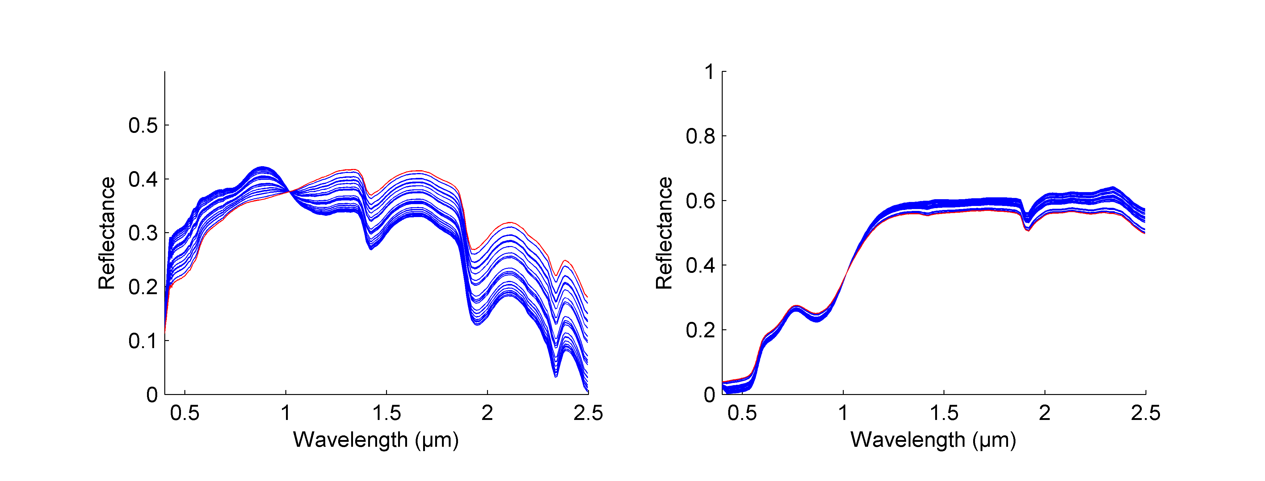
Figure 1: Range of admissible solution for two endmember spectra : construction concrete (left) and red brick (right). The actual endmember (red lines) are mixed according (1) under the constraints in (3) with random proportions to obtain $P=2500$ pixels. $50$ admissible solutions (blue lines) of the BSS problems in (6) are generated using [40].

III Bayesian model

III-A Likelihood

The linear mixing model defined in (1) and the statistical properties in (2) of the noise vector ${\mathbf{n}}_{p}$ result in a conditionally Gaussian distribution for the observation of the $p$th pixel: $\mathbf{y}_{p}|{\mathbf{M}},{\mathbb{a}}_{p},\sigma^{2}\sim\mathcal{N}\left({\mathbf{M}}{\mathbb{a}}_{p},\sigma^{2}\textbf{I}_{L}\right)$. Therefore, the likelihood function of $\mathbf{y}_{p}$ can be expressed as

$$f\left(\mathbf{y}_{p}\big{|}{\mathbf{M}},{\mathbb{a}}_{p},\sigma^{2}\right)=\left(\frac{1}{2\pi\sigma^{2}}\right)^{\frac{L}{2}}\exp\left[-\frac{\left\|\mathbf{y}_{p}-{\mathbf{M}}{\mathbb{a}}_{p}\right\|^{2}}{2\sigma^{2}}\right],$$ (8)

where $\left\|\mathbb{x}\right\|=\left({\mathbb{x}^{T}\mathbb{x}}\right)^{\frac{1}{2}}$ is the $\ell_{2}$ norm. Assuming the independence between the noise sequences ${\mathbf{n}}_{p}$ ($p=1,\ldots,P$), the likelihood function of all the observations $\mathbf{Y}$ is:

$$f\left(\mathbf{Y}\big{|}{\mathbf{M}},{\mathbb{A}},\sigma^{2}\right)=\prod_{p=1}^{P}f\left(\mathbf{y}_{p}\big{|}{\mathbf{M}},{\mathbb{a}}_{p},\sigma^{2}\right).$$ (9)

III-B Prior model for the endmember spectra

III-B1 Dimensionality reduction

It is interesting to note that the unobserved matrix ${\mathbf{X}}={\mathbf{M}}{\mathbb{A}}=\mathbf{Y}-{\mathbb{N}}$ is rank deficient under the linear model (1). More precisely, the set

$$\mathcal{S}_{{\mathbf{M}}}=\left\{{\mathbf{x}}\in\mathds{R}^{L};\ {\mathbf{x}}=\sum_{r=1}^{R}\lambda_{r}{\mathbf{m}}_{r},\ \sum_{r=1}^{R}\lambda_{r}=1,\ \lambda_{r}\geq 0\right\}$$ (10)

is a $(R-1)$-dimensional convex polytope of $\mathds{R}^{L}$ whose vertices are the $R$ endmember spectra ${\mathbf{m}}_{r}$ ($r=1,\ldots,R$) to be recovered. Consequently, in the noise-free case, ${\mathbf{X}}$ can be represented in a suitable lower-dimensional subset ${\mathcal{V}}_{K}$ of $\mathds{R}^{K}$ without lost of information.

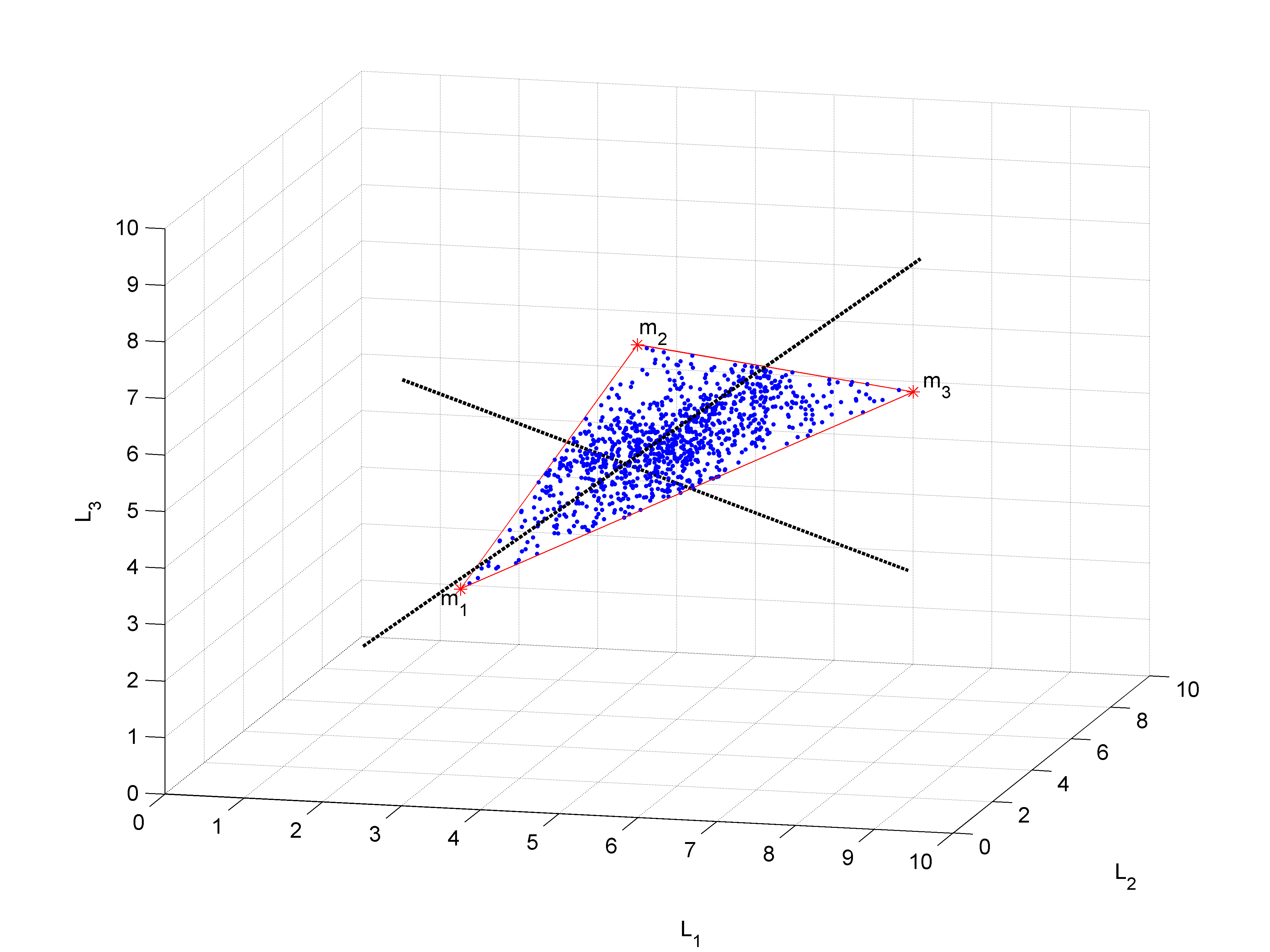
Figure 2: Example of hyperspectral data observed in $3$ spectral bands. The mixed pixels (blue points) belong to the $R$-dimensional convex polytope $\mathcal{S}_{{\mathbf{M}}}$ (red lines) whose vertices are the endmembers spectra ${\mathbf{m}}_{1},\ldots,{\mathbf{m}}_{R}$ (red stars). The first two principal axes estimated by a PCA appear in dashed lines and define the projection subset ${\mathcal{V}}_{K}$.

To illustrate this property, $P=1000$ pixels resulting from a noise-free mixture of $R=3$ endmembers are represented in Fig. 2. As noted in [4], this dimensionality reduction is a common step of the LSMA, adopted by numerous EEAs, such as N-FINDR [9] or PPI [8]. Similarly, we propose to estimate the projection ${\mathbf{t}}_{r}$ ($r=1,\ldots,R$) of the endmember spectra ${\mathbf{m}}_{r}$ in the subspace ${\mathcal{V}}_{K}$. The identification of this subspace can be achieved via a standard dimension reduction procedure. In the sequel, we propose to define ${\mathcal{V}}_{K}$ as the subspace spanned by $K$ orthogonal axes ${\mathbf{v}}_{1},\ldots,{\mathbf{v}}_{K}$ identified by a principal component analysis (PCA) on the observations $\mathbf{Y}$ [41]:

$${\mathcal{V}}_{K}=\textrm{span}\left({\mathbf{v}}_{1},\ldots,{\mathbf{v}}_{K}\right).$$ (11)

The first two principal axes are identified in Fig. 2 for the synthetic hyperspectral data. In the following paragraph, the PCA is described. Note however that this PCA-based dimension reduction step can be easily replaced by other projection techniques, such as the maximum noise fraction (MNF) transform [42] that has been considered in paragraph V-D.

III-B2 PCA projection

The $L\times L$ empirical covariance matrix $\boldsymbol{\Upsilon}$ of the data $\mathbf{Y}$ is given by:

$$\boldsymbol{\Upsilon}=\frac{1}{P}\sum_{p=1}^{P}\left(\mathbf{y}_{p}-\bar{\mathbf{y}}\right)\left(\mathbf{y}_{p}-\bar{\mathbf{y}}\right)^{T}$$ (12)

where $\bar{\mathbf{y}}$ is the empirical mean:

$$\bar{\mathbf{y}}=\frac{1}{P}\sum_{p=1}^{P}\mathbf{y}_{p}.$$ (13)

Let

$$\left\{\begin{split}{\mathbf{D}}&=\mathrm{diag}\left(\lambda_{1},\ldots,\lambda_{K}\right),\\ \mathbf{V}&=\left[{\mathbf{v}}_{1},\ldots,{\mathbf{v}}_{K}\right]^{T}\end{split}\right.$$ (14)

denote respectively the diagonal matrix of the $K$ highest eigenvalues and the corresponding eigenvector matrix of $\boldsymbol{\Upsilon}$. The PCA projection ${\mathbf{t}}_{r}\in\mathds{R}^{K}$ of the endmember spectrum ${\mathbf{m}}_{r}\in\mathds{R}^{L}$ is obtained as follows:

$${\mathbf{t}}_{r}={\mathbf{P}}\left({\mathbf{m}}_{r}-\bar{\mathbf{y}}\right),$$ (15)

with ${\mathbf{P}}=\mathbf{D}^{-\frac{1}{2}}{\mathbf{V}}$. Equivalently,

$${\mathbf{m}}_{r}={\mathbf{U}}{\mathbf{t}}_{r}+\bar{\mathbf{y}},$$ (16)

with ${\mathbf{U}}={\mathbf{V}}^{{\dagger}}{\mathbf{D}}^{\frac{1}{2}}$ where ${\mathbf{V}}^{{\dagger}}\triangleq\left({\mathbf{V}}^{T}{\mathbf{V}}\right)^{-1}{\mathbf{V}}^{T}$ is the pseudo-inverse of ${\mathbf{V}}$. Note that in the subspace ${\mathcal{V}}_{R-1}$ obtained for $K=R-1$, the vectors $\left\{{\mathbf{t}}_{r}\right\}_{r=1,\ldots,R}$ form a simplex that standard EEAs such as N-FINDR [9], MVT [11] and ICE [27] try to recover. In this paper, we estimate the vertices ${\mathbf{t}}_{r}$ ($r=1,\ldots,R$) of this simplex using a Bayesian approach. The Bayesian prior distributions for the projections ${\mathbf{t}}_{r}$ ($r=1,\ldots,R$) are introduced in the following paragraph.

III-B3 Prior distribution for the projected spectra

All the elements of the subspace ${\mathcal{V}}_{K}$ may not be appropriate projected spectra according to (15). Indeed, the $K\times 1$ vector ${\mathbf{t}}_{r}$ has to ensure non-negativity constraints (5) of the corresponding reconstructed $L\times 1$ spectra ${\mathbf{m}}_{r}$. For each endmember ${\mathbf{m}}_{r}$, straightforward computations establish that for any $r=1,\ldots,R$

$$\left\{m_{l,r}\geq 0,\ \forall l=1,\ldots,L\right\}\quad\Leftrightarrow\quad\left\{{\mathbf{t}}_{r}\in\mathcal{T}_{r}\right\},$$ (17)

where the set $\mathcal{T}_{r}\subset{\mathcal{V}}_{K}$ is defined by the following $L$ inequalities

$$\mathcal{T}_{r}=\left\{{\mathbf{t}}_{r};\bar{y}_{l}+\sum_{k=1}^{K}u_{l,k}t_{k,r}\geq 0,l=1,\ldots,L\right\},$$ (18)

with $\bar{\mathbf{y}}=\left[\bar{y}_{1},\ldots,\bar{y}_{L}\right]^{T}$ and ${\mathbf{U}}=\left[u_{l,k}\right]$. A conjugate multivariate Gaussian distribution (MGD) ${\mathcal{N}}_{\mathcal{T}_{r}}\left({\mathbf{e}}_{r},s^{2}_{r}\textbf{I}_{K}\right)$ truncated on the set $\mathcal{T}_{r}$ is chosen as prior distribution for ${\mathbf{t}}_{r}$. The probability density function (pdf) $\phi_{\mathcal{T}_{r}}\left(\cdot\right)$ of this truncated MGD is defined by:

$$\phi_{\mathcal{T}_{r}}\left({\mathbf{t}}_{r}\big{|}{\mathbf{e}}_{r},s^{2}_{r}\textbf{I}_{K}\right)\propto\phi\left({\mathbf{t}}_{r}\big{|}{\mathbf{e}}_{r},s^{2}_{r}\textbf{I}_{K}\right)\textbf{1}_{\mathcal{T}_{r}}\left({\mathbf{t}}_{r}\right),$$ (19)

where $\propto$ stands for “proportional to”, $\phi\left(\cdot|{\mathbf{u}},{\mathbf{W}}\right)$ is the pdf of the standard MGD $\mathcal{N}\left({\mathbf{u}},{\mathbf{W}}\right)$ with mean vector ${\mathbf{u}}$ and covariance matrix ${\mathbf{W}}$, and $\textbf{1}_{\mathcal{T}_{r}}\left(\cdot\right)$ is the indicator function on the set ${\mathcal{T}_{r}}$:

$$\textbf{1}_{\mathcal{T}_{r}}\left({\mathbf{x}}\right)=\left\{\begin{array}[]{ll}1,&\hbox{if ${\mathbf{x}}\in{\mathcal{T}_{r}}$ };\\ 0,&\hbox{overwise.}\end{array}\right.$$ (20)

The normalizing constant $K_{\mathcal{T}_{r}}\left({\mathbf{e}}_{r},s^{2}_{r}\textbf{I}_{K}\right)$ in (19) is defined as follows:

$$K_{\mathcal{T}_{r}}\left({\mathbf{e}}_{r},s^{2}_{r}\textbf{I}_{K}\right)=\int_{\mathcal{T}_{r}}\phi\left({\mathbf{x}}|{\mathbf{e}}_{r},s^{2}_{r}\textbf{I}_{K}\right)d{\mathbf{x}}.$$ (21)

This paper proposes to choose the mean vectors ${\mathbf{e}}_{r}$ ($r=1,\ldots,R$) in (19) as the projected spectra of pure components previously identified by EEA, e.g., N-FINDR. The variances $s^{2}_{r}$ ($r=1,\ldots,R$) reflect the degree of confidence given to this prior information. When no additional knowledge is available, these variances are fixed to large values: $s^{2}_{1}=\ldots=s^{2}_{R}=50$.

By assuming a priori independence of the vectors ${\mathbf{t}}_{r}$ ($r=1,\ldots,R$), the prior distribution for the projected endmember matrix ${\mathbf{T}}=\left[{\mathbf{t}}_{1},\ldots,{\mathbf{t}}_{R}\right]$ is

$$f\left({\mathbf{T}}\mid{\mathbf{E}},{\mathbf{s}}^{2}\right)=\prod_{r=1}^{R}\phi_{\mathcal{T}_{r}}\left({\mathbf{t}}_{r}\big{|}{\mathbf{e}}_{r},s^{2}_{r}\textbf{I}_{K}\right),$$ (22)

where ${\mathbf{E}}=\left[{\mathbf{e}}_{1},\ldots,{\mathbf{e}}_{R}\right]$ and ${\mathbf{s}}^{2}=\left[s^{2}_{1},\ldots,s^{2}_{R}\right]$.

III-C Abundance prior

For each observed pixel $p$, with the full additivity constraint in (3), the abundance vectors ${\mathbb{a}}_{p}$ ($p=1,\ldots,P$) can be rewritten as

$${\mathbb{a}}_{p}=\left[\begin{array}[]{c}{\mathbb{c}}_{p}\\ a_{p,R}\\ \end{array}\right]\qquad\text{with }\qquad{\mathbb{c}}_{p}=\left[\begin{array}[]{c}a_{p,1}\\ \vdots\\ a_{p,R-1}\\ \end{array}\right],$$

and $a_{p,R}=1-\sum_{r=1}^{R-1}a_{p,r}$. Following the model in [18], the priors chosen for ${\mathbb{c}}_{p}$ ($p=1,\ldots,P$) are uniform distributions on the simplex $\mathcal{S}$ defined by:

$$\mathcal{S}=\left\{{\mathbb{c}}_{p};\ \left\|{\mathbb{c}}_{p}\right\|_{1}\leq 1\ \text{and }{\mathbb{c}}_{p}\succeq\boldsymbol{0}\right\}.$$ (23)

Choosing this prior distribution for ${\mathbb{c}}_{p}$ (${p}=1,\ldots,P$) is equivalent to electing a Dirichlet distribution ${\mathcal{D}}\left(1,\ldots,1\right)$, i.e a uniform distribution on ${\mathcal{A}}$ defined in (4), as prior distribution for the full abundance vector ${\mathbb{a}}_{p}$ [43, Appendix A]. However, the proposed reparametrization will prove to be well adapted to the Gibbs sampling strategy introduced in Section IV.

Under the assumption of statistical independence between the abundance vectors ${\mathbb{c}}_{p}$ ($p=1,\ldots,P$), the full prior distribution for partial abundance matrix ${\mathbb{C}}=\left[{\mathbb{c}}_{1},\ldots,{\mathbb{c}}_{P}\right]^{T}$ can be written

$$f\left({\mathbb{C}}\right)\propto\prod_{p=1}^{P}\textbf{1}_{\mathcal{S}}\left({\mathbb{c}}_{p}\right).$$ (24)

As noted in [18], the uniform prior distribution reflects the lack of a priori knowledge about the abundance vector. Moreover, for the BSS problem here, this imposes a strong constraint on the size of the simplex to be recovered. As demonstrated in the Appendix, among two a priori equiprobable solutions of the BSS problem, this uniform prior allows one to favor a posteriori the solution corresponding to the polytope in the projection subset ${\mathcal{V}}_{K}$ with smallest volume. This property has also been exploited in [11].

III-D Noise variance prior

A conjugate prior is chosen for $\sigma^{2}$:

$$\sigma^{2}\left|{\nu},{\gamma}\right.\sim\mathcal{IG}\left(\frac{\nu}{2},\frac{\gamma}{2}\right),$$ (25)

where $\mathcal{IG}\left(\frac{\nu}{2},\frac{\gamma}{2}\right)$ denotes the inverse-gamma distribution with parameters $\frac{\nu}{2}$ and $\frac{\gamma}{2}$. As in previous works ([44] and [45]), the hyperparameter $\nu$ will be fixed to $\nu=2$. On the other hand, $\gamma$ will be a random and adjustable hyperparameter, whose prior distribution is defined below.

III-E Prior distribution for hyperparameter $\gamma$

The prior for $\gamma$ is a non-informative Jeffreys’ prior [46] which reflects the lack of knowledge regarding this hyperparameter:

$$f\left(\gamma\right)\propto\frac{1}{\gamma}\textbf{1}_{\mathbb{R}^{+}}\left(\gamma\right).$$ (26)

III-F Posterior distribution

The posterior distribution of the unknown parameter vector $\boldsymbol{\theta}=\left\{{\mathbb{C}},{\mathbf{T}},\sigma^{2}\right\}$ can be computed from marginalization using the following hierarchical structure

$$f(\boldsymbol{\theta}|\mathbf{Y})=\int f(\boldsymbol{\theta},\gamma|\mathbf{Y})d\gamma\propto\int f(\mathbf{Y}|\boldsymbol{\theta})f(\boldsymbol{\theta}|\gamma)f(\gamma)d\gamma,$$ (27)

where $f\left(\mathbf{Y}\big{|}\boldsymbol{\theta}\right)$ and $f\left(\gamma\right)$ are defined in (9) and (26) respectively. Moreover, under the assumption of a priori independence between ${\mathbb{C}}$, ${\mathbf{T}}$ and $\sigma^{2}$, the following result can be obtained:

$$f\left(\boldsymbol{\theta}\big{|}\gamma\right)=f\left({\mathbb{C}}\right)f\left({\mathbf{T}}\mid{\mathbf{E}},{\mathbf{s}}^{2}\right)f\left(\sigma^{2}\mid\nu,\gamma\right),$$ (28)

where $f\left({\mathbb{C}}\mid{\mathbf{E}},{\mathbf{s}}^{2}\right)$, $f\left({\mathbf{T}}\right)$ and $f\left(\sigma^{2}\mid\nu,\gamma\right)$ have been defined in Eq.’s (24), (22) and (25), respectively.

This hierarchical structure allows one to integrate out the hyperparameter $\gamma$ from the joint distribution $f\left(\boldsymbol{\theta},\gamma|\mathbf{Y}\right)$, yielding:

$$\begin{split}f&\left({\mathbb{C}},{\mathbf{T}},\sigma^{2}\big{|}\mathbf{Y}\right)\propto\prod_{p=1}^{P}\textbf{1}_{\mathcal{S}}\left({\mathbb{c}}_{p}\right)\\ &\times\prod_{r=1}^{R}\exp\left[-\frac{\left\|{\mathbf{t}}_{r}-{\mathbf{e}}_{r}\right\|^{2}}{2s^{2}_{r}}\right]\textbf{1}_{\mathcal{T}_{r}}\left({\mathbf{t}}_{r}\right)\\ &\times\prod_{p=1}^{P}\left[\left(\frac{1}{\sigma^{2}}\right)^{\frac{L}{2}+1}\exp\left(-\frac{\left\|\mathbf{y}_{p}-\left({\mathbf{U}}{\mathbf{T}}+\bar{\mathbf{y}}\right){\mathbb{a}}_{p}\right\|^{2}}{2\sigma^{2}}\right)\right].\end{split}$$ (29)

Deriving the Bayesian estimators (e.g., MMSE or MAP) from the posterior distribution in (29) remains intractable. In such case, it is very common to use Markov chain Monte Carlo (MCMC) methods to generate samples asymptotically distributed according to the posterior distribution. The Bayesian estimators can then be approximated using these samples. The next section studies a Gibbs sampling strategy allowing one to generate samples distributed according to (29).

IV Gibbs sampler

Random samples (denoted by ${\cdot}^{(t)}$ where $t$ is the iteration index) can be drawn from $f\left({\mathbb{C}},{\mathbf{T}},\sigma^{2}\mid\mathbf{Y}\right)$ using a Gibbs sampler [47]. This MCMC technique consists of generating samples $\left\{{\mathbb{C}}^{(t)},{\mathbf{T}}^{(t)},{\boldsymbol{\sigma}}^{2(t)}\right\}$ distributed according to the conditional posterior distributions of each parameter.

    Algorithm 1:
Gibbs sampling algorithm for LSMA

IV-A Sampling from $f\left({\mathbb{C}}|{\mathbf{T}},\sigma^{2},\mathbf{Y}\right)$

Straightforward computations yield for each observation:

$$f\left({\mathbb{c}}_{p}\left|{\mathbf{T}},\sigma^{2},\mathbf{y}_{p}\right.\right)\\ \propto\exp\left[-\frac{\left({\mathbb{c}}_{p}-\boldsymbol{\upsilon}_{p}\right)^{T}{\boldsymbol{\Sigma}}^{-1}_{p}\left({\mathbb{c}}_{p}-\boldsymbol{\upsilon}_{p}\right)}{2}\right]\textbf{1}_{\mathcal{S}}\left({\mathbb{c}}_{p}\right),$$ (30)

where:

$$\left\{\begin{split}{\boldsymbol{\Sigma}}_{p}&=\left[\left({\mathbf{M}}_{\text{-}R}-{\mathbf{m}}_{R}{\boldsymbol{1}}_{R-1}^{T}\right)^{T}{\boldsymbol{\Sigma}}_{\textrm{n}}^{-1}\left({\mathbf{M}}_{\text{-}R}-{\mathbf{m}}_{R}{\boldsymbol{1}}_{R-1}^{T}\right)\right]^{-1},\\ {\boldsymbol{\upsilon}}_{p}&={\boldsymbol{\Sigma}}_{p}\left[\left({\mathbf{M}}_{\text{-}R}-{\mathbf{m}}_{R}{\boldsymbol{1}}_{R-1}^{T}\right)^{T}{\boldsymbol{\Sigma}}_{\textrm{n}}^{-1}\left(\mathbf{y}_{p}-{\mathbf{m}}_{R}\right)\right],\end{split}\right.$$ (31)

with ${\boldsymbol{\Sigma}}_{\textrm{n}}^{-1}=\frac{1}{\sigma^{2}}\textbf{I}_{L}$, ${\boldsymbol{1}}_{R-1}=[1,\ldots,1]^{T}\in\mathbb{R}^{R-1}$ and where ${\mathbf{M}}_{\text{-}R}$ denotes the matrix ${\mathbf{M}}$ whose $R$th column has been removed. As a consequence, ${\mathbb{c}}_{p}\big{|}{\mathbf{T}},\sigma^{2},\mathbf{y}_{p}$ is distributed according to an MGD truncated on the simplex $\mathcal{S}$ in (23):

$${\mathbb{c}}_{p}\left|{\mathbf{T}},\sigma^{2},\mathbf{y}_{p}\right.\sim\mathcal{N}_{\mathcal{S}}\left(\boldsymbol{\upsilon}_{p},\boldsymbol{\Sigma}_{p}\right).$$ (32)

Note that samples can be drawn from an MGD truncated on a simplex using efficient Monte Carlo simulation strategies such as described in [48].

IV-B Sampling from $f\left({\mathbf{T}}|{\mathbb{C}},\sigma^{2},\mathbf{Y}\right)$

Define ${\mathbf{T}}_{\text{-}r}$ as the matrix ${\mathbf{T}}$ whose $r$th column has been removed. Then the conditional posterior distribution of ${\mathbf{t}}_{r}$ ($r=1,\ldots,R$) is:

$$f\left({\mathbf{t}}_{r}|{\mathbf{T}}_{\text{-}r},{\mathbb{c}}_{r},\sigma^{2},\mathbf{Y}\right)\propto\\ \exp\left[-\frac{1}{2}\left({\mathbf{t}}_{r}-\boldsymbol{\tau}_{r}\right)^{T}\boldsymbol{\Lambda}_{r}^{-1}\left({\mathbf{t}}_{r}-\boldsymbol{\tau}_{r}\right)\right]\textbf{1}_{\mathcal{T}_{r}}\left({\mathbf{t}}_{r}\right),$$ (33)

with

$$\left\{\begin{split}{\boldsymbol{\Lambda}}_{r}&=\left[\sum_{p=1}^{P}a_{p,r}^{2}{\mathbf{U}}^{T}{\boldsymbol{\Sigma}}_{\textrm{n}}^{-1}{\mathbf{U}}+\frac{1}{s^{2}_{r}}\textbf{I}_{K}\right]^{-1},\\ {\boldsymbol{\tau}}_{r}&={\boldsymbol{\Lambda}}_{r}\left[\sum_{p=1}^{P}a_{p,r}^{2}{\mathbf{U}}^{T}{\boldsymbol{\Sigma}}_{\textrm{n}}^{-1}\boldsymbol{\epsilon}_{p,r}+\frac{1}{s^{2}_{r}}{\mathbf{e}}_{r}\right],\end{split}\right.$$ (34)

and

$$\boldsymbol{\epsilon}_{p,r}=\mathbf{y}_{p}-a_{p,r}\bar{\mathbf{y}}-\sum_{j\neq r}a_{p,j}{\mathbf{m}}_{j}.$$ (35)

Note that ${\mathbf{m}}_{j}={\mathbf{U}}{\mathbf{t}}_{j}+\bar{\mathbf{y}}$. As a consequence, the posterior distribution of ${\mathbf{t}}_{r}$ is the following truncated MGD:

$${\mathbf{t}}_{r}\mid{\mathbf{T}}_{\text{-}r},{\mathbb{c}}_{r},\sigma^{2},\mathbf{Y}\sim{\mathcal{N}}_{\mathcal{T}_{r}}\left(\boldsymbol{\tau}_{r},\boldsymbol{\Lambda}_{r}\right).$$ (36)

Generating vectors distributed according to this distribution is a difficult task, mainly due to the truncation on the subset $\mathcal{T}_{r}$. An alternative consists of generating each component $t_{k,r}$ of ${\mathbf{t}}_{r}$ conditionally upon the others ${\mathbf{t}}_{\text{-}k,r}=\left\{t_{j,r}\right\}_{j\neq k}$. More precisely, by denoting ${\mathcal{U}}_{k}^{+}=\left\{l;u_{l,k}>0\right\}$, ${\mathcal{U}}_{k}^{-}=\left\{l;u_{l,k}<0\right\}$ and $\varepsilon_{l,k,r}=\bar{y}_{l}+\sum_{j\neq k}u_{l,j}t_{j,r}$, one can write

$$t_{k,r}|{\mathbf{t}}_{\text{-}k,r},{\mathbf{T}}_{\text{-}r},{\mathbb{c}}_{r},\sigma^{2},\mathbf{Y}\sim{\mathcal{N}}_{\left[t_{k,r}^{-},t_{k,r}^{+}\right]}\left(w_{{k},{r}},z^{2}_{{k},{r}}\right),$$ (37)

with

$$\left\{\begin{split}t_{k,r}^{-}&=\max_{l\in{\mathcal{U}}_{k}^{+}}-\frac{\varepsilon_{l,k,r}}{u_{l,k}},\\ t_{k,r}^{+}&=\min_{l\in{\mathcal{U}}_{k}^{-}}-\frac{\varepsilon_{l,k,r}}{u_{l,k}},\\ \end{split}\right.$$ (38)

and where $w_{{k},{r}}$ and $z^{2}_{{k},{r}}$ are the conditional mean and variance respectively, derived from the partitioned mean vector and covariance matrix [49, p. 324] (see [48] for similar computations). Generating samples distributed according to the two-sided truncated Gaussian distribution in (37) can be easily achieved with the algorithm described in [50].

IV-C Sampling from $f\left(\sigma^{2}|{\mathbb{C}},{\mathbf{T}},\mathbf{Y}\right)$

The conditional distribution of $\sigma^{2}|{\mathbb{C}},{\mathbf{T}},\mathbf{Y}$ is the following inverse Gamma distribution:

$$\sigma^{2}|{\mathbb{C}},{\mathbf{T}},\mathbf{Y}\sim\mathcal{IG}\left(\frac{PL}{2},\frac{1}{2}\sum_{p=1}^{P}\left\|\mathbf{y}_{p}-{\mathbf{M}}{\mathbb{a}}_{p}\right\|^{2}\right).$$ (39)

Simulating according to this inverse Gamma distribution can be achieved using a Gamma variate generator (see [51, Ch. 9] and [43, Appendix A]).

To summarize, the hyperparameters that have to be fixed at the beginning of the algorithm are the following: $\nu=2$, $s^{2}_{1}=\ldots=s^{2}_{R}=50$ and $\left\{{\mathbf{e}}_{r}\right\}_{r=1,\ldots,R}$ are set to projected spectra identified by a standard EEA (e.g., N-FINDR).

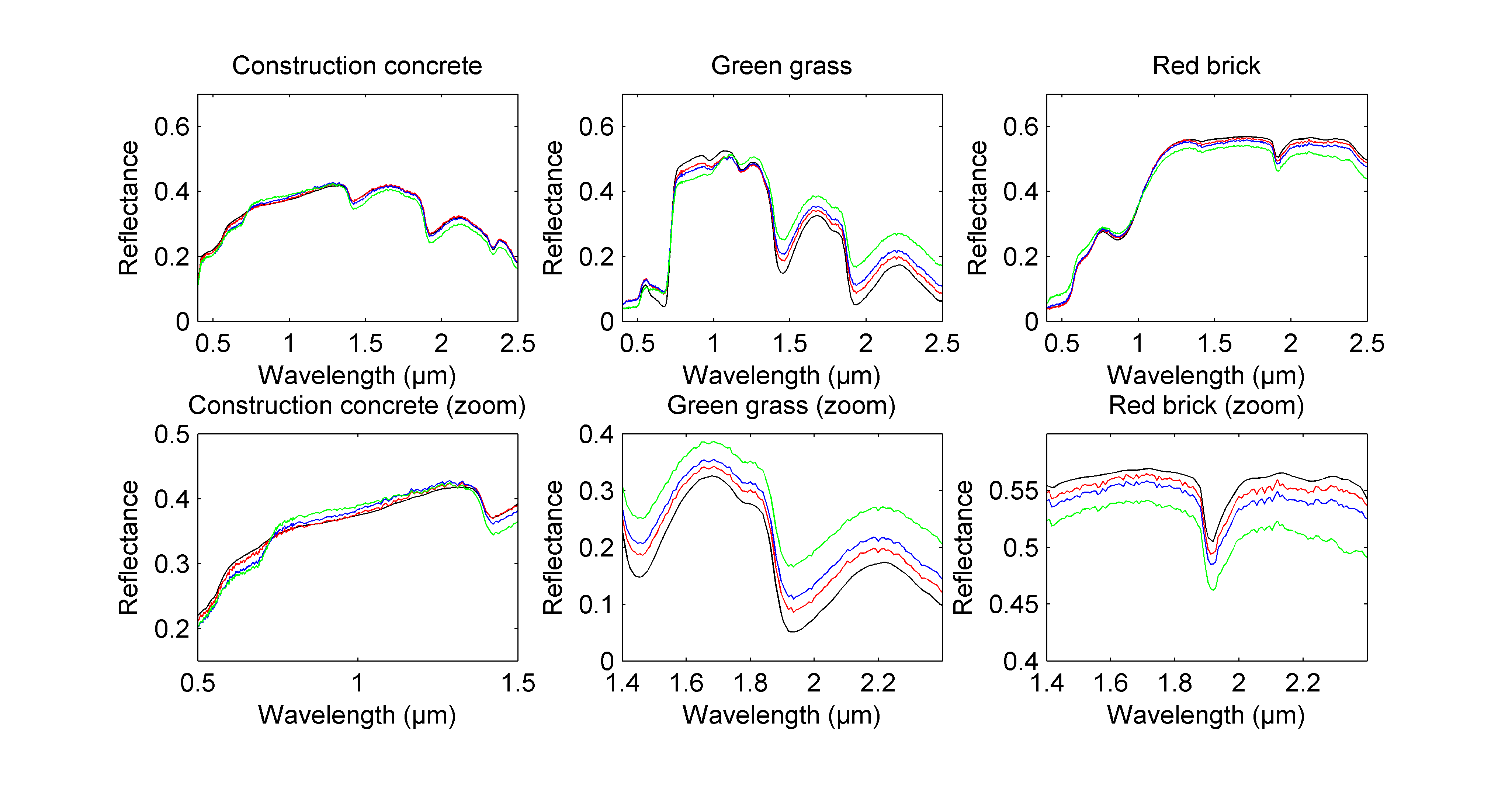
Figure 3: Actual endmembers (black lines), endmembers estimated by N-FINDR (blue lines), endmembers estimated by VCA (green lines) and endmembers estimated by proposed approach (red lines).

V Simulations on synthetic data

To illustrate the accuracy of the proposed algorithm, simulations are conducted on a $100\times 100$ synthetic image. This hyperspectral image is composed of three different regions with $R=3$ pure materials representative of a sub-urban scene: construction concrete, green grass and red brick. The spectra of these endmembers have been extracted from the spectral libraries distributed with the ENVI software [52] and are represented in Fig. 3 (top, black lines). The reflectances are observed in $L=413$ spectral bands ranging from $0.4\mu m$ to $2.5\mu m$. These $R=3$ components have been mixed with proportions that have been randomly generated according to truncated MGDs reflecting the means and variances reported in Table I. The generated abundance maps have been depicted in Fig. 5 (top) in gray scale where a white (resp. black) pixel stands for the presence (resp. absence) of the material. The signal-to-noise ratio has been tuned to $\textrm{SNR}_{\textrm{dB}}=15$dB.

TABLE I: Abundance means and variances of each endmember in each region of the $100\times 100$ hyperspectral image.

	Region $\#1$		Region $\#2$		Region $\#3$
	mean	var.	mean	var.	mean	var.
Endm. #1	$0.60$	$0.01$	$0.25$	$0.01$	$0.25$	$0.02$
Endm. #2	$0.20$	$0.02$	$0.50$	$0.01$	$0.15$	$0.005$
Endm. #3	$0.20$	$0.01$	$0.25$	$0.02$	$0.60$	$0.02$

V-A Endmember spectrum estimation

The resulting hyperspectral data have been unmixed by the proposed algorithm. First, the space ${\mathcal{V}}_{K}$ in (11) has been identified by PCA as discussed in paragraph III-B2. The hidden mean vectors ${\mathbf{e}}_{r}$ ($r=1,\ldots,R$) of the normal distributions in (19) have been chosen as the PCA projections of endmembers previously identified by N-FINDR. The hidden variances $s^{2}_{r}$ have all been chosen equal to $s^{2}_{1}=\ldots=s^{2}_{R}=50$ to obtain vague priors (i.e. large variances). The Gibbs sampler has been run with $N_{\textrm{MC}}=1300$ iterations, including $N_{\textrm{bi}}=300$ burn-in iterations. The MMSE estimates of the abundance vectors ${\mathbb{a}}_{p}$ ($p=1,\ldots,P$) and the projected spectra ${\mathbf{t}}_{r}$ ($r=1,\ldots,R$) have been approximated by computing empirical averages over the last computed outputs of the sampler $\left\{{\mathbb{a}}_{r}^{(t)}\right\}_{t=1,\ldots,N_{\textrm{MC}}}$ and $\left\{{\mathbf{t}}_{r}^{(t)}\right\}_{t=1,\ldots,N_{\textrm{MC}}}$, following the MMSE principle:

$$\begin{split}\hat{{\mathbf{x}}}_{\textrm{MMSE}}&=\mathrm{E}\left[{\mathbf{x}}|{\mathbf{y}}\right]\\ &\approx\frac{1}{N_{\textrm{MC}}-N_{\textrm{bi}}}\sum_{t=N_{\textrm{bi}}+1}^{N_{\textrm{MC}}}{\mathbf{x}}^{(t)}.\end{split}$$ (40)

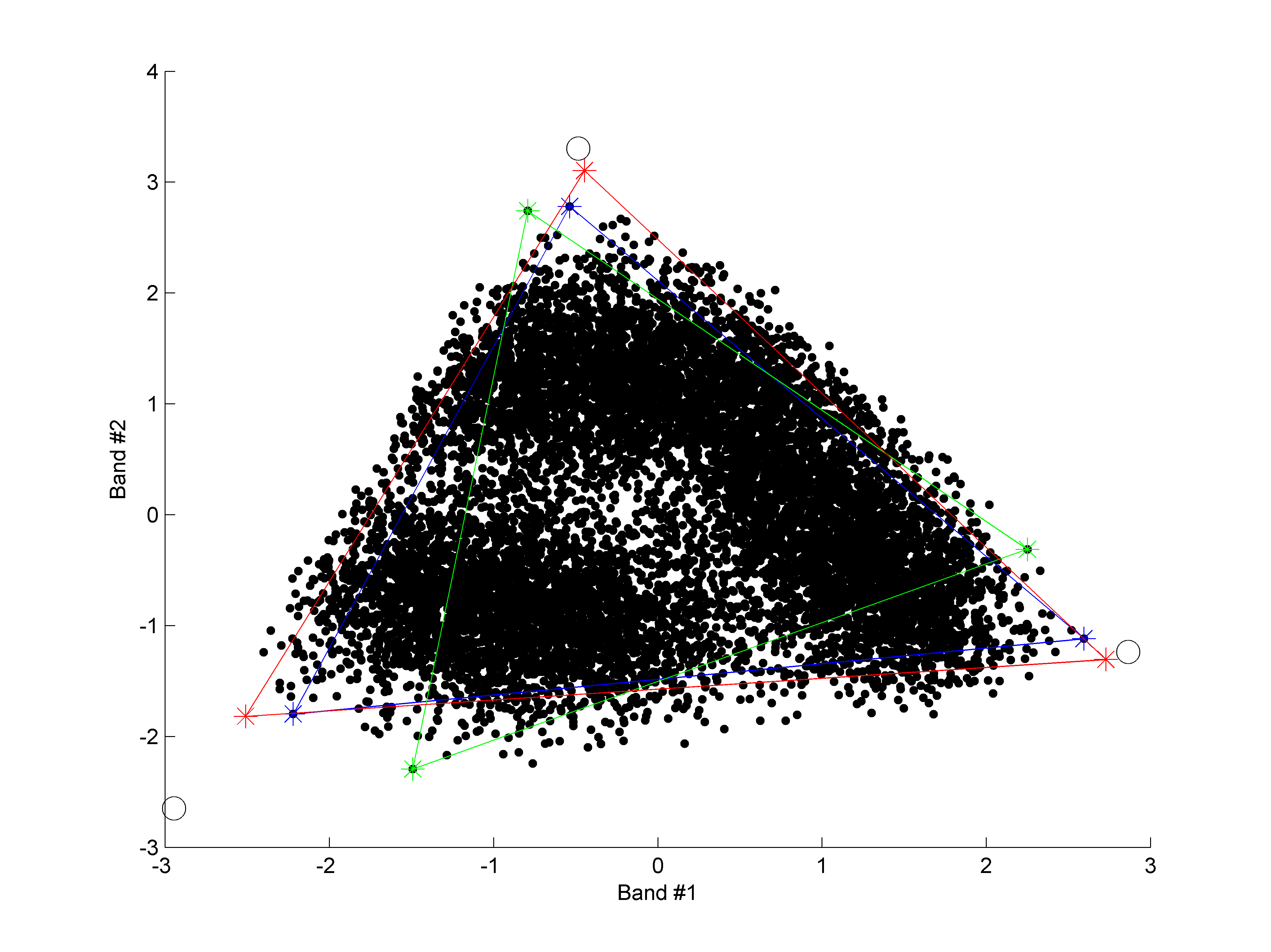
Figure 4: Scatter plot in the lower-dimensional space ${\mathcal{V}}_{2}$: projected dataset (black points), actual endmembers (black circles), endmembers estimated by N-FINDR (blue stars), endmembers estimated by VCA (green stars) and endmembers estimated by proposed approach (red stars). All pixel spectra do not lie inside ground truth simplex due to simulated measurement noise.

The corresponding endmember spectra estimated by the proposed algorithm are depicted in Fig. 3 (top, red lines). The proposed algorithm clearly outperforms N-FINDR and VCA, as shown in Fig. 3. The scatter plot in Fig. 4 provides additional insight. The N-FINDR and VCA algorithms assume the presence of pure pixels in the data. However, as none of these pixels are pure, N-FINDR and VCA provide poorer results than the proposed joint Bayesian algorithm. To illustrate this point, the performances of the different algorithms have been compared via two criteria. First, the mean square errors (MSEs)

$$\textrm{MSE}_{r}^{2}=\left\|\hat{{\mathbf{m}}_{r}}-{{\mathbf{m}}_{r}}\right\|^{2},\quad r=1,\ldots,R$$ (41)

are good quality indicators for the estimates. In addition, another metric frequently encountered in hyperspectral imagery literature, known as the spectral angle distance (SAD), has been considered. The SAD measures the angle between the actual and the corresponding estimated spectrum:

$$\textrm{SAD}_{r}=\arccos\left(\frac{\langle\hat{{\mathbf{m}}_{r}},{{\mathbf{m}}_{r}}\rangle}{\left\|\hat{{\mathbf{m}}_{r}}\right\|\left\|{{\mathbf{m}}_{r}}\right\|}\right),$$ (42)

where $\langle\cdot,\cdot\rangle$ stands for the scalar product. These performance criteria computed for the endmember spectra estimated by the different algorithm have been reported in Table III. They show that the proposed method performs significantly better than the others. The computation times required by each of these algorithms are reported in Table II for a unoptimized MATLAB 2007b 32bit implementation on a $2.2$GHz Intel Core 2. Obviously, the complexity of the VCA and N-FINDR methods are lower than the proposed approach. Note however that, contrary to the joint Bayesian procedure, these standard EEA have to be coupled with an abundance estimation algorithm. Moreover they only provide point estimates of the endmember spectra. Note finally that the computational complexity of N-FINDR, because it is combinatorial, increases drastically with the number of pixels and endmembers.

TABLE II: Computational times of VCA, N-FINDR and the proposed Bayesian method for unmixing $P=32\times 32$ pixels.

	Bayesian	VCA	N-FINDR
Times (s)	$3250$	$1$	$23$

TABLE III: Performance comparison between VCA, N-FINDR and the proposed Bayesian method: $\textrm{MSE}^{2}$ and SAD $(\times 10^{-1})$ between the actual and the estimated endmember spectra.

		End.	Bayesian		VCA		N-FINDR
			$\textrm{MSE}^{2}$	SAM	$\textrm{MSE}^{2}$	SAM	$\textrm{MSE}^{2}$	SAM
$\textrm{SNR}=5{\textrm{dB}}$	$R=3$	#1	$1.70$	$0.63$	$17.80$	$1.91$	$2.69$	$0.75$
		#2	$6.56$	$1.49$	$10.87$	$1.80$	$10.87$	$1.80$
		#3	$2.70$	$0.59$	$12.71$	$1.40$	$2.94$	$0.60$
	$R=5$	#1	$0.70$	$0.01$	$64.47$	$3.93$	$49.16$	$3.46$
		#2	$1.05$	$0.49$	$47.21$	$3.13$	$15.46$	$2.07$
		#3	$1.04$	$0.49$	$17.11$	$1.81$	$17.11$	$1.81$
		#4	$1.05$	$0.49$	$13.43$	$1.23$	$6.92$	$0.79$
		#5	$1.04$	$0.49$	$16.12$	$1.45$	$4.92$	$0.88$
$\textrm{SNR}=15{\textrm{dB}}$	$R=3$	#1	$0.10$	$0.15$	$1.29$	$0.48$	$0.54$	$0.33$
		#2	$2.68$	$0.92$	$15.59$	$2.12$	$5.19$	$1.26$
		#3	$0.16$	$0.12$	$4.35$	$0.71$	$0.57$	$0.22$
	$R=5$	#1	$0.12$	$0.17$	$0.70$	$0.40$	$0.70$	$0.40$
		#2	$0.97$	$0.52$	$11.34$	$1.44$	$10.57$	$1.68$
		#3	$0.26$	$0.22$	$4.07$	$0.72$	$0.43$	$0.25$
		#4	$0.40$	$0.15$	$2.36$	$0.44$	$7.67$	$0.47$
		#5	$0.24$	$0.18$	$1.54$	$0.43$	$2.93$	$0.60$
$\textrm{SNR}=25{\textrm{dB}}$	$R=3$	#1	$0.05$	$0.09$	$1.14$	$0.52$	$1.14$	$0.52$
		#2	$2.19$	$0.83$	$5.65$	$1.33$	$5.65$	$1.33$
		#3	$0.17$	$0.14$	$0.66$	$0.22$	$0.66$	$0.22$
	$R=5$	#1	$0.42$	$0.29$	$7.62$	$1.32$	$7.62$	$1.32$
		#2	$0.37$	$0.34$	$27.16$	$2.23$	$20.66$	$2.40$
		#3	$0.46$	$0.29$	$6.75$	$1.10$	$2.26$	$0.65$
		#4	$0.07$	$0.09$	$10.02$	$0.93$	$10.88$	$0.70$
		#5	$0.35$	$0.20$	$3.73$	$0.61$	$3.71$	$0.62$

V-B Abundance estimation

The MMSE estimates of the abundance vectors for the $P=10^{4}$ pixels of the image have been computed following the MMSE principle in (40)

$$\hat{{\mathbb{a}}}_{p}=\frac{1}{N_{\textrm{MC}}-N_{\textrm{bi}}}\sum_{t=N_{\textrm{bi}}+1}^{N_{\textrm{MC}}}{\mathbb{a}}_{p}^{(t)}.$$ (43)

The corresponding estimated abundance maps are depicted in Fig. 5 (bottom) and are clearly in good agreement with the simulated maps (top).

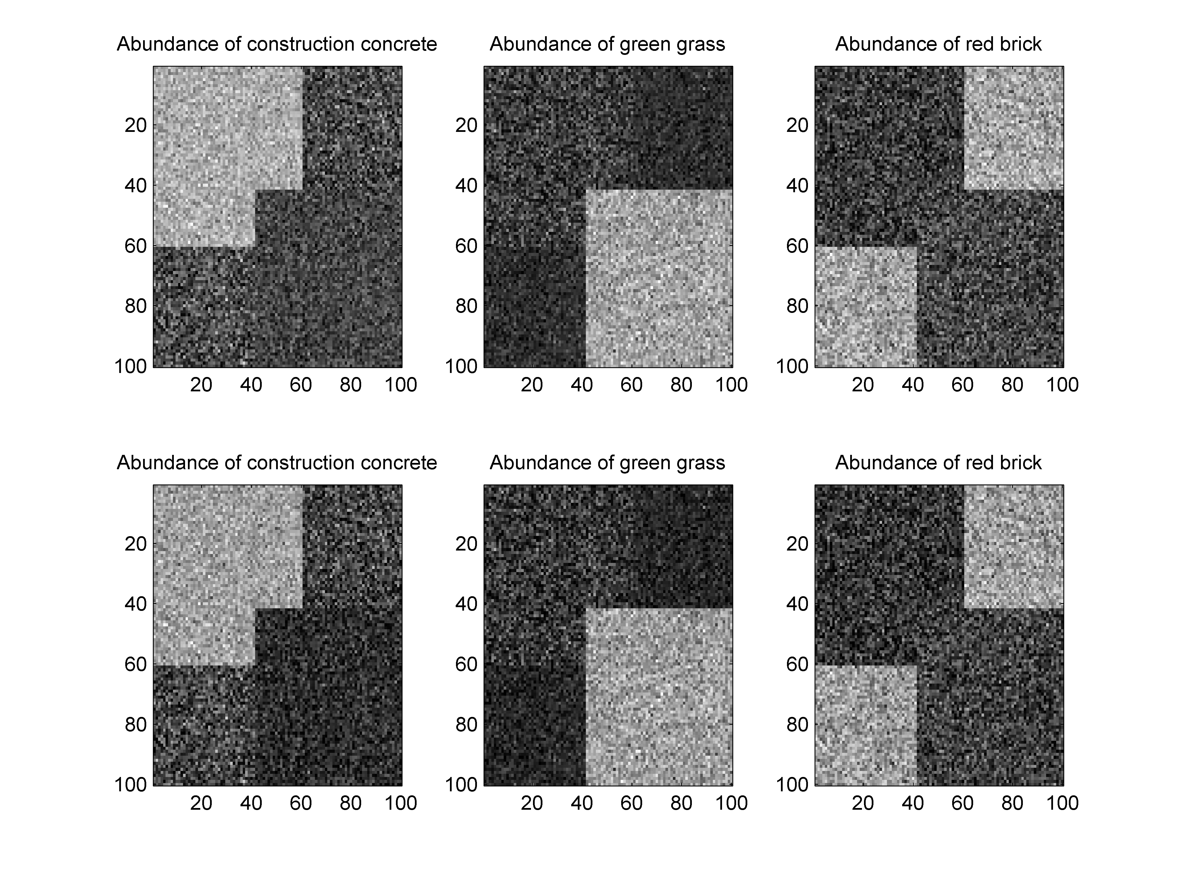
Figure 5: Top: actual endmember abundance maps. Bottom: estimated endmember abundance maps.

Note that the proposed Bayesian estimation provides the joint posterior distribution of the unknown parameters. Specifically, these posteriors allow one to derive confidence intervals regarding the parameters of interest. For instance, the posterior distributions of the abundance coefficients is depicted in Fig. 6 for the pixel #100. Note that these estimated posteriors are in good agreement with the actual values of ${\mathbb{a}}_{100}$ depicted in red dotted lines.

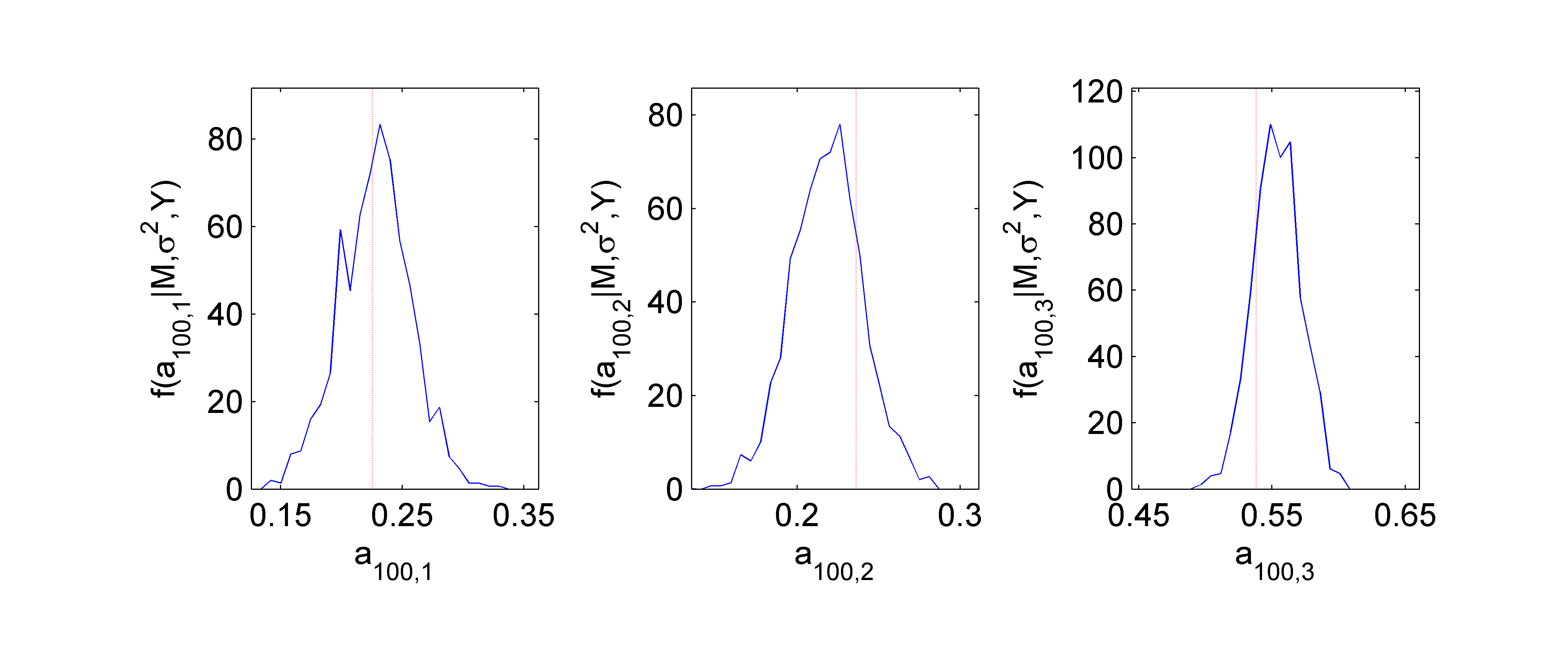
Figure 6: Posterior distributions of $a_{p,r}$ ($r=1,\ldots,3$). The actual values are depicted in red dotted lines.

These results have been compared with estimates provided by the N-FINDR or VCA algorithms, coupled with an abundance estimation procedure based on the Fully Constrained Least-Squares (FCLS) approach proposed by Heinz et al. [16]. The global abundance MSEs have been computed following:

$$\textrm{GMSE}_{r}^{2}=\sum_{p=1}^{P}\left(\hat{a}_{p,r}-a_{p,r}\right)^{2},$$ (44)

where $\hat{a}_{p,r}$ is the estimated abundance coefficient of the material #$r$ in the pixel #$p$. These performance measures have been reported in Table IV and confirm the accuracy of the proposed Bayesian estimation method. Moreover, note that neither N-FINDR nor VCA are able to provide confidence measures as those depicted in Fig 6.

TABLE IV: Performance comparison between VCA, N-FINDR and the proposed Bayesian method: $\textrm{GMSE}^{2}$ between the actual and the estimated abundance maps.

	Bayesian	VCA	N-FINDR
Endm. #1	$25.68$	$57.43$	$30.66$
Endm. #2	$29.97$	$74.48$	$46.45$
Endm. #3	$3.19$	$83.02$	$11.22$

V-C Other simulation scenarios

Simulations have also been conducted with different noise levels ($\textrm{SNR}_{\textrm{dB}}=5\textrm{dB},~{}25\textrm{dB}$) and when $R=3$ or $R=5$ endmembers are involved in the mixture. Estimation performances for the VCA and N-FINDR algorithms, as well as the proposed approach, have been summarized in Table III. These results expressed in terms of MSE and SAD corroborate the effectiveness of our Bayesian estimation procedure.

V-D Robustness to non-i.i.d noise models

In this paragraph, we illustrate the robustness of the proposed algorithm with respect to violation of the i.i.d. noise assumption. More precisely, a so-called Gaussian shaped noise inspired by [53] has been considered. The noise correlation matrix ${\boldsymbol{\Sigma}}_{\textrm{n}}=\textrm{diag}\left(\sigma^{2}_{1},\ldots,\sigma^{2}_{L}\right)$ is designed such that its diagonal elements $\sigma^{2}_{l}$ ($l=1,\ldots,L$) follow a Gaussian shape centered at band $L/2$

$$\sigma^{2}_{l}=\sigma^{2}\exp\left[-\frac{\left(l-L/2\right)^{2}}{2\eta^{2}}\right].$$ (45)

The parameter $\sigma^{2}$ can be tuned to choose the SNR whereas the parameter $\eta$ adjusts the shape width ($\eta\rightarrow\infty$ corresponds to i.i.d. noise). For this simulation, the parameters $\sigma^{2}$ and $\eta$ have been fixed to $1.0\times 10^{2}$ and $50$ respectively, leading to a noise level of $\textrm{SNR}_{\textrm{dB}}=15\textrm{dB}$.

When the noise is not i.i.d., dimensionality reduction methods based on eigen-decomposition of observed data correlation matrix $\boldsymbol{\Upsilon}$ introduced in (12) can be inefficient. In this case, other hyperspectral subspace identification methods have to be considered. Here the PCA-based dimension reduction step introduced in paragraph III-B2 was replaced by two techniques: the well-known MNF transform [42] approach and the more recently introduced HySime algorithm [53]. Both of them requires noise covariance matrix ${\boldsymbol{\Sigma}}_{\textrm{n}}$ estimation, which was implemented following [53]. The estimation performances for the proposed Bayesian estimation procedure coupled with MNF or HySime are reported in Table V and compared with VCA and N-FINDR. These results show that the proposed method i) can be easily used with other dimension reduction procedures, and ii) is quite robust to the i.i.d. noise assumption.

TABLE V: Performance comparison between VCA, N-FINDR and the proposed Bayesian method in presence of Gaussian shaped noise: $\textrm{MSE}^{2}$ and SAD $(\times 10^{-1})$ between the actual and the estimated endmember spectra.

	MNF + Bayesian		HySime + Bayesian		VCA		N-FINDR
	$\textrm{MSE}^{2}$	SAD	$\textrm{MSE}^{2}$	SAD	$\textrm{MSE}^{2}$	SAD	$\textrm{MSE}^{2}$	SAD
Endm. #1	$0.26$	$0.25$	$0.42$	$0.31$	$1.11$	$0.46$	$1.11$	$0.46$
Endm. #2	$1.99$	$0.79$	$4.35$	$1.16$	$5.78$	$1.33$	$5.78$	$1.33$
Endm. #3	$0.33$	$0.19$	$0.57$	$0.22$	$1.94$	$0.41$	$2.19$	$0.43$

VI Real data

This section illustrates the proposed algorithm on real hyperspectral data. The considered hyperspectral image was acquired over Moffett Field (CA, USA) in 1997 by the JPL spectro-imager AVIRIS [54]. This image has been used in many works to illustrate hyperspectral signal processing algorithms [55, 56].

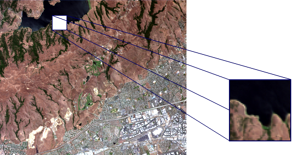
Figure 7: Real hyperspectral data: Moffett Field image acquired by AVIRIS in 1997 (left) and the region of interest (right) represented in synthetic colors.

A $50\times 50$ sub-image depicted in Fig. 7 (right) has been unmixed using the proposed Bayesian approach. The number of endmembers has been estimated as in [18]. More precisely, we retain the first $R-1$ eigenvalues identified by PCA that capture $95\%$ of the energy contained into the dataset. As detailed in III-B1, we use also PCA to choose the subset ${\mathcal{V}}_{R-1}$ defined in (11). After a short burn-in period $N_{\textrm{bi}}=50$, estimates of the parameters of interest are computing following the MMSE principle in (40) with $N_{r}=450$. The $R=3$ endmembers recovered by the proposed joint Bayesian LSMA algorithm are depicted in Fig. 8 (top). These endmember spectra are represented in $L=189$ spectral bands after removing the water absorption bands. These endmembers are characteristic of the coastal area that appears in the image: vegetation, water and soil. The corresponding abundance maps, shown Fig. 8 (bottom), are in agreement with the previous results presented in [18].

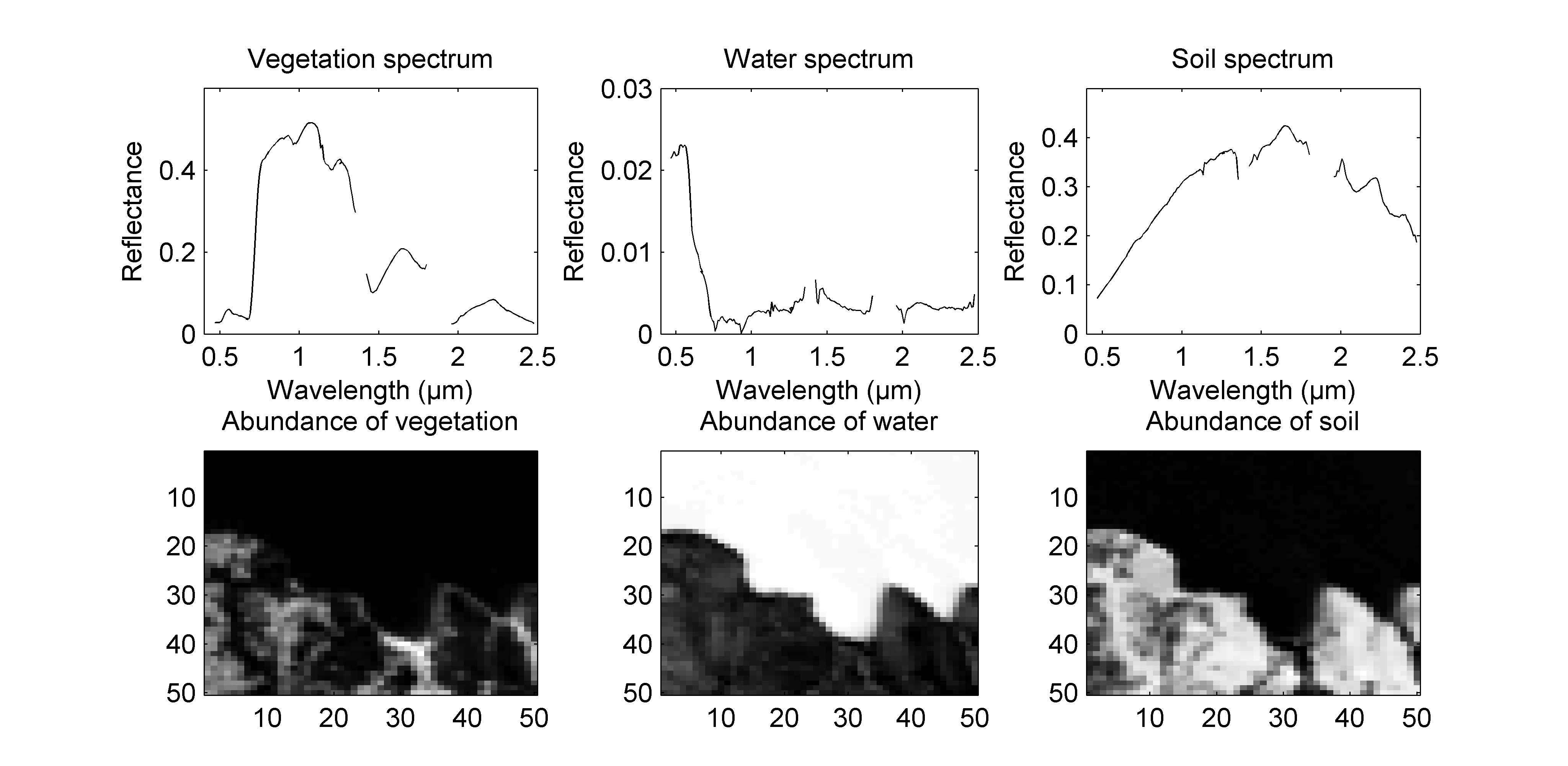
Figure 8: Top: the $R=3$ endmember spectra estimated by the algorithm. Bottom: the corresponding abundance maps (black (respectively, white) means absence (respectively, presence) of the material).

VII Conclusions

This paper presented a Bayesian model as well as an MCMC algorithm for unsupervised unmixing of hyperspectral images, i.e. estimating the endmember spectra in the observed scene and their respective abundances for each pixel. Appropriate priors were chosen for the abundance vectors to ensure non-negativity and sum-to-one constraints inherent to the linear mixing model. Instead of estimating the endmember spectral signatures in the observation space, we proposed to estimate their projections onto a suitable subspace. In this subspace, which can be identified by a standard dimension reduction technique such as PCA, MNF and HySime, these projections were assigned priors that satisfy positivity constraints of the reconstructed endmember spectra. Due to the complexity of the posterior distribution, a Gibbs sampling scheme was proposed to generate samples asymptotically distributed according to this posterior. The available samples were then used to approximate the Bayesian estimators for the different parameters of interest. Results of simulations conducted on synthetic and real hyperspectral image illustrated the accuracy of the proposed Bayesian method when compared with other algorithms from the literature. An interesting open question is whether one can improve performance further by folding the intrinsic dimension $K$ of the projection subspace ${\mathcal{V}}_{K}$ into the Bayesian framework, e.g., by applying Bayesian PCA or Bayesian latent variable models. This question is a topic of our current research. While this paper introduced a Bayesian method in the context of hyperspectral unmixing, the method can also be used for other unmixing applications, such as blind source separation, that satisfy positivity and sum-to-one constraints.

[On the choice of uniform distributions as prior distributions for ${\mathbb{a}}_{r}$ and the size of the simplex solution of the BSS problem]

In this appendix, we show that choosing uniform distributions as priors for the abundance vectors allows one to favor a posteriori, among two a priori equiprobable polytopes that are admissible solutions of the BSS problem, the solution corresponding to the smallest polytope.

Property: Let ${\mathbf{M}}^{(1)}$ and ${\mathbf{M}}^{(2)}$ be two $R$-dimensional convex polytopes of $\mathds{R}^{L}$ that are admissible solutions of the BSS constrained problem, i.e.

$$\begin{array}[]{c}\exists{\mathbb{A}}^{(1)}=\left[{\mathbb{a}}_{1}^{(1)},\ldots,{\mathbb{a}}_{R}^{(1)}\right]^{T}\subset{\mathcal{A}}^{R},\\ \exists{\mathbb{A}}^{(2)}=\left[{\mathbb{a}}_{1}^{(2)},\ldots,{\mathbb{a}}_{R}^{(2)}\right]^{T}\subset{\mathcal{A}}^{R},\\ \end{array}$$ (46)

such as $\mathbf{Y}={\mathbf{M}}^{(1)}{\mathbb{A}}^{(1)}={\mathbf{M}}^{(2)}{\mathbb{A}}^{(2)}$ where ${\mathcal{A}}$ has been defined in (4). Then

$$\begin{split}&f\left({{\mathbf{M}}}^{(1)}|\mathbf{Y}\right)\geq f\left({{\mathbf{M}}}^{(2)}|\mathbf{Y}\right)\\ \Leftrightarrow&\\ &\textrm{vol}\left(\mathcal{S}_{{{\mathbf{M}}}^{(1)}}\right)\leq\textrm{vol}\left(\mathcal{S}_{{{\mathbf{M}}}^{(2)}}\right),\end{split}$$ (47)

where $\textrm{vol}\left(\mathcal{S}_{{{\mathbf{M}}}^{(i)}}\right)$ stands for the volume of the polytope $\mathcal{S}_{{{\mathbf{M}}}^{(i)}}\subset\mathds{R}^{L}$ introduced in (10) whose vertices are the columns of ${\mathbf{M}}^{(i)}$.

Proof: First note that, in absence of noise, as $\mathbf{y}_{p}={\mathbf{M}}{\mathbb{a}}_{p}$,

$${\mathbb{a}}_{p}\sim{\mathcal{U}}\left({\mathcal{A}}\right)\Leftrightarrow\mathbf{y}_{p}|{\mathbf{M}}\sim{\mathcal{U}}\left(\mathcal{S}_{{\mathbf{M}}}\right),$$ (48)

where ${\mathcal{U}}\left(\cdot\right)$ stands for the uniform distribution.

Consequently,

$$f\left(\mathbf{Y}|{\mathbf{M}}\right)=\left[\frac{1}{\mathrm{vol}\left(\mathcal{S}_{{\mathbf{M}}}\right)}\right]^{P}\prod_{p}^{P}\textbf{1}_{\mathcal{S}_{{\mathbf{M}}}}\left(\mathbf{y}_{p}\right),$$ (49)

which can be simplified by

$$f\left(\mathbf{Y}|{\mathbf{M}}\right)=\left[\frac{1}{\mathrm{vol}\left(\mathcal{S}_{{\mathbf{M}}}\right)}\right]^{P},$$ (50)

since, by definition, the observed pixels $\mathbf{y}_{p}$ ($p=1,\ldots,P$) belong to the solution polytope $\mathcal{S}_{{\mathbf{M}}}$. Moreover, Bayes’ paradigm allows one to state:

$$f\left({\mathbf{M}}|\mathbf{Y}\right)=\frac{f\left(\mathbf{Y}|{\mathbf{M}}\right)f\left({\mathbf{M}}\right)}{f\left(\mathbf{Y}\right)}.$$ (51)

Since the two solutions ${{\mathbf{M}}^{(1)}}$ and ${{\mathbf{M}}^{(2)}}$ are a priori equiprobable, from (50), it yields:

$$\frac{f\left({{\mathbf{M}}^{(1)}}|\mathbf{Y}\right)}{f\left({{\mathbf{M}}^{(2)}}|\mathbf{Y}\right)}=\left[\frac{\mathrm{vol}\left(\mathcal{S}_{{{\mathbf{M}}}^{(2)}}\right)}{\mathrm{vol}\left(\mathcal{S}_{{{\mathbf{M}}}^{(1)}}\right)}\right]^{P}.$$ (52)

It follows (47).

$\blacksquare$

Note that the equiprobability assumption underlying the solutions $\mathcal{S}_{{{\mathbf{M}}}^{(2)}}$ and $\mathcal{S}_{{{\mathbf{M}}}^{(2)}}$ is not a too restrictive hypothesis. Indeed if the variances $s^{2}_{r}$ ($r=1,\ldots,R$) had been chosen such that the prior distribution in (22) is sufficiently flat, then:

$$f\left({\mathbf{M}}^{(1)}\right)\approx f\left({\mathbf{M}}^{(2)}\right).$$ (53)

Note also that the projection of the polytope $\mathcal{S}_{{{\mathbf{M}}}^{(i)}}$ onto the subset ${\mathcal{V}}_{R-1}\subset\mathds{R}^{R-1}$ is the simplex $\mathcal{S}_{{{\mathbf{T}}}^{(i)}}$ whose vertices are the columns of ${\mathbf{T}}^{(i)}$.

References

- [1] C.-I Chang, Hyperspectral Imaging: Techniques for Spectral detection and classification. New York: Kluwer, 2003.
- [2] J. Plaza, R. Pérez, A. Plaza, P. Martínez, and D. Valencia, “Mapping oil spills on sea water using spectral mixture analysis of hyperspectral image data,” in Chemical and Biological Standoff Detection III, J. O. Jensen and J.-M. Thériault, Eds., vol. 5995. SPIE, 2005, pp. 79–86.
- [3] D. Manolakis, C. Siracusa, and G. Shaw, “Hyperspectral subpixel target detection using the linear mixing model,” IEEE Trans. Geosci. and Remote Sensing, vol. 39, no. 7, pp. 1392–1409, July 2001.
- [4] N. Keshava and J. F. Mustard, “Spectral unmixing,” IEEE Signal Processing Magazine, pp. 44– 57, Jan. 2002.
- [5] R. B. Singer and T. B. McCord, “Mars: Large scale mixing of bright and dark surface materials and implications for analysis of spectral reflectance,” in Proc. 10th Lunar and Planetary Sci. Conf., March 1979, pp. 1835–1848.
- [6] B. W. Hapke, “Bidirectional reflectance spectroscopy. I. Theory,” J. Geophys. Res., vol. 86, pp. 3039– 3054, 1981.
- [7] P. E. Johnson, M. O. Smith, S. Taylor-George, and J. B. Adams, “A semiempirical method for analysis of the reflectance spectra of binary mineral mixtures,” J. Geophys. Res., vol. 88, pp. 3557–3561, 1983.
- [8] J. Boardman, “Automating spectral unmixing of AVIRIS data using convex geometry concepts,” in Summaries 4th Annu. JPL Airborne Geoscience Workshop, vol. 1. Washington, D.C.: JPL Pub., 1993, pp. 11–14.
- [9] M. Winter, “Fast autonomous spectral end-member determination in hyperspectral data,” in Proc. 13th Int. Conf. on Applied Geologic Remote Sensing, vol. 2, Vancouver, April 1999, pp. 337–344.
- [10] J. M. Nascimento and J. M. Bioucas-Dias, “Vertex component analysis: A fast algorithm to unmix hyperspectral data,” IEEE Trans. Geosci. and Remote Sensing, vol. 43, no. 4, pp. 898–910, April 2005.
- [11] M. Craig, “Minimum volume transforms for remotely sensed data,” IEEE Trans. Geosci. and Remote Sensing, pp. 542–552, 1994.
- [12] J. H. Bowles, P. J. Palmadesso, J. A. Antoniades, M. M. Baumback, and L. J. Rickard, “Use of filter vectors and fast convex set methods in hyperspectral analysis,” in Infrared Spaceborne Remote Sensing III, M. Strojnik and B. F. Andresen, Eds., vol. 2553, no. 148. SPIE, Sept. 1995, pp. 148–157.
- [13] A. Plaza, P. Martinez, R. Perez, and J. Plaza, “A quantitative and comparative analysis of endmember extraction algorithms from hyperspectral data,” IEEE Trans. Geosci. and Remote Sensing, vol. 42, no. 3, pp. 650–663, March 2004.
- [14] P. J. Martinez, R. M. Pérez, A. Plaza, P. L. Aguilar, M. C. Cantero, and J. Plaza, “Endmember extraction algorithms from hyperspectral images,” Annals of Geophysics, vol. 49, no. 1, pp. 93–101, Feb. 2006.
- [15] N. Keshava, J. P. Kerekes, D. G. Manolakis, and G. A. Shaw, “Algorithm taxonomy for hyperspectral unmixing,” in Algorithms for Multispectral, Hyperspectral, and Ultraspectral Imagery VI, S. S. Shen and M. R. Descour, Eds., vol. 4049, no. 1. SPIE, 2000, pp. 42–63.
- [16] D. C. Heinz and C.-I Chang, “Fully constrained least-squares linear spectral mixture analysis method for material quantification in hyperspectral imagery,” IEEE Trans. Geosci. and Remote Sensing, vol. 29, no. 3, pp. 529–545, March 2001.
- [17] J. Settle, “On the relationship between spectral unmixing and subspace projection,” IEEE Trans. Geosci. and Remote Sensing, vol. 34, no. 4, pp. 1045–1046, July 1996.
- [18] N. Dobigeon, J.-Y. Tourneret, and C.-I Chang, “Semi-supervised linear spectral unmixing using a hierarchical Bayesian model for hyperspectral imagery,” IEEE Trans. Signal Processing, vol. 56, no. 7, pp. 2684–2695, July 2008.
- [19] P. Common, C. Jutten, and J. Herault, “Blind separation of sources. Part II: problems statement,” Signal Processing, vol. 24, no. 1, pp. 11–20, July 1991.
- [20] T. W. Lee, Independent component analysis: theory and applications. Hingham, MA: Kluwer Academic Publishers, 1998.
- [21] J. Bayliss, J. A. Gualtieri, and R. Cromp, “Analyzing hyperspectral data with independent component analysis,” in Proc. AIPR Workshop Exploiting New Image Sources and Sensors, J. M. Selander, Ed., vol. 3240. Washington, D.C.: SPIE, 1998, pp. 133–143.
- [22] N. Dobigeon and V. Achard, “Performance comparison of geometric and statistical methods for endmembers extraction in hyperspectral imagery,” in Image and Signal Processing for Remote Sensing XI, L. Bruzzone, Ed., vol. 5982, no. 1. SPIE, Oct. 2005, pp. 335–344.
- [23] J. M. P. Nascimento and J. M. Bioucas-Dias, “Does independent component analysis play a role in unmixing hyperspectral data?” IEEE Trans. Geosci. and Remote Sensing, vol. 43, no. 1, pp. 175–187, Jan. 2005.
- [24] J. M. Nascimento and J. M. Bioucas-Dias, “Hyperspectral unmixing algorithm via dependent component analysis,” vol. 43, no. 4, July 2007, pp. 4033–4036.
- [25] P. Paatero and U. Tapper, “Positive matrix factorization: a non-negative factor model with optimal utilization of error estimates of data values,” Environmetrics, vol. 5, pp. 111–126, 1994.
- [26] P. Sajda, S. Du, T. R. Brown, R. Stoyanova, D. C. Shungu, X. Mao, and L. C. Parra, “Nonnegative matrix factorization for rapid recovery of constituent spectra in magnetic resonance chemical shift imaging of the brain,” IEEE Trans. Medical Imaging, vol. 23, no. 12, pp. 1453–1465, 2004.
- [27] M. Berman, H. Kiiveri, R. Lagerstrom, A. Ernst, R. Dunne, and J. F. Huntington, “ICE: A statistical approach to identifying endmembers in hyperspectral images,” IEEE Trans. Geosci. and Remote Sensing, vol. 42, no. 10, pp. 2085–2095, Oct. 2004.
- [28] L. Miao and H. Qi, “Endmember extraction from highly mixed data using minimum volume constrained nonnegative matrix factorization,” IEEE Trans. Geosci. and Remote Sensing, vol. 45, no. 3, pp. 765– 777, March 2007.
- [29] D. B. Rowe, “A Bayesian approach to blind source separation,” J. of Interdisciplinary Mathematics, vol. 5, no. 1, pp. 49–76, 2002.
- [30] C. Févotte and S. J. Godsill, “A Bayesian approach for blind separation of sparse sources,” IEEE Trans. Audio, Speech, Language Processing, vol. 14, no. 6, pp. 2174–2188, Nov. 2006.
- [31] S. Moussaoui, D. Brie, A. Mohammad-Djafari, and C. Carteret, “Separation of non-negative mixture of non-negative sources using a Bayesian approach and MCMC sampling,” IEEE Trans. Signal Processing, vol. 54, no. 11, pp. 4133–4145, Nov. 2006.
- [32] N. Dobigeon, S. Moussaoui, and J.-Y. Tourneret, “Blind unmixing of linear mixtures using a hierarchical bayesian model. Application to spectroscopic signal analysis,” in Proc. IEEE-SP Workshop Stat. and Signal Processing, Madison, USA, Aug. 2007, pp. 79–83.
- [33] J. C. Harsanyi and C.-I Chang, “Hyperspectral image classification and dimensionality reduction: An orthogonal subspace projection approach,” IEEE Trans. Geosci. and Remote Sensing, vol. 32, no. 4, pp. 779–785, July 1994.
- [34] C.-I Chang, “Further results on relationship between spectral unmixing and subspace projection,” IEEE Trans. Geosci. and Remote Sensing, vol. 36, no. 3, pp. 1030–1032, May 1998.
- [35] C.-I Chang, X.-L. Zhao, M. L. G. Althouse, and J. J. Pan, “Least squares subspace projection approach to mixed pixel classification for hyperspectral images,” IEEE Trans. Geosci. and Remote Sensing, vol. 36, no. 3, pp. 898–912, May 1998.
- [36] N. Dobigeon and J.-Y. Tourneret, “Bayesian sampling of structured noise covariance matrix for hyperspectral imagery,” University of Toulouse, Tech. Rep., Dec. 2008. [Online]. Available: http://dobigeon.perso.enseeiht.fr/publis.html
- [37] J. Li, “Wavelet-based feature extraction for improved endmember abundance estimation in linear unmixing of hyperspectral signals,” IEEE Trans. Geosci. and Remote Sensing, vol. 42, no. 3, pp. 644–649, March 2004.
- [38] C.-I Chang and B. Ji, “Weighted abundance-constrained linear spectral mixture analysis,” IEEE Trans. Geosci. and Remote Sensing, vol. 44, no. 2, pp. 378–388, Feb. 2001.
- [39] T. Veit, J. Idier, and S. Moussaoui, “Rééchantillonnage de l’échelle dans les algorithmes MCMC pour les problèmes inverses bilinéaires,” Traitement du Signal, 2009, to appear.
- [40] S. Moussaoui, D. Brie, and J. Idier, “Non-negative source separation: range of admissible solutions and conditions for the uniqueness of the solution,” in Proc. IEEE Int. Conf. Acoust., Speech, and Signal Processing (ICASSP), vol. 5, Philadelphia, USA, March 2005, pp. 289–292.
- [41] I. T. Jolliffe, Principal Component Analysis. New York: Springer-Verlag, 1986.
- [42] A. A. Green, M. Berman, P. Switzer, and M. D. Craig, “A transformation for ordering multispectral data in terms of image quality with implications for noise removal,” IEEE Trans. Geosci. and Remote Sensing, vol. 26, no. 1, pp. 65–74, Jan. 1988.
- [43] C. P. Robert, The Bayesian Choice: from Decision-Theoretic Motivations to Computational Implementation, 2nd ed., ser. Springer Texts in Statistics. New York: Springer-Verlag, 2007.
- [44] E. Punskaya, C. Andrieu, A. Doucet, and W. Fitzgerald, “Bayesian curve fitting using MCMC with applications to signal segmentation,” IEEE Trans. Signal Processing, vol. 50, no. 3, pp. 747–758, March 2002.
- [45] N. Dobigeon, J.-Y. Tourneret, and M. Davy, “Joint segmentation of piecewise constant autoregressive processes by using a hierarchical model and a Bayesian sampling approach,” IEEE Trans. Signal Processing, vol. 55, no. 4, pp. 1251–1263, April 2007.
- [46] H. Jeffreys, Theory of Probability, 3rd ed. London: Oxford University Press, 1961.
- [47] C. P. Robert and G. Casella, Monte Carlo Statistical Methods. New York: Springer-Verlag, 1999.
- [48] N. Dobigeon and J.-Y. Tourneret, “Efficient sampling according to a multivariate Gaussian distribution truncated on a simplex,” IRIT/ENSEEIHT/TéSA, Tech. Rep., March 2007. [Online]. Available: http://dobigeon.perso.enseeiht.fr/publis.html
- [49] S. M. Kay, Fundamentals of Statistical Signal Processing: Estimation theory. Englewood Cliffs NJ: Prentice Hall, 1993.
- [50] C. P. Robert, “Simulation of truncated normal variables,” Statistics and Computing, vol. 5, pp. 121–125, 1995.
- [51] L. Devroye, Non-Uniform Random Variate Generation. New York: Springer-Verlag, 1986.
- [52] RSI (Research Systems Inc.), ENVI User’s guide Version 4.0, Boulder, CO 80301 USA, Sept. 2003.
- [53] J. M. Bioucas-Dias and J. M. P. Nascimento, “Hyperspectral subspace identification,” IEEE Trans. Geosci. and Remote Sensing, vol. 46, no. 8, pp. 2435–2445, Aug. 2008.
- [54] AVIRIS Free Data. (2006) Jet Propulsion Lab. (JPL). California Inst. Technol., Pasadena, CA. [Online]. Available: http://aviris.jpl.nasa.gov/html/aviris.freedata.html
- [55] E. Christophe, D. Léger, and C. Mailhes, “Quality criteria benchmark for hyperspectral imagery,” IEEE Trans. Geosci. and Remote Sensing, vol. 43, no. 9, pp. 2103–2114, Sept. 2005.
- [56] T. Akgun, Y. Altunbasak, and R. M. Mersereau, “Super-resolution reconstruction of hyperspectral images,” IEEE Trans. Image Processing, vol. 14, no. 11, pp. 1860–1875, Nov. 2005.