Chemical evolution of the Galactic bulge as traced by
microlensed dwarf and subgiant stars.

Abstract

Aims. Our aims are twofold. First we aim to evaluate the robustness and accuracy of stellar parameters and detailed elemental abundances that can be derived from high-resolution spectroscopic observations of microlensed dwarf and subgiant stars. We then aim to use microlensed dwarf and subgiant stars to investigate the abundance structure and chemical evolution of the Milky Way Bulge. Contrary to the cool giant stars, with their extremely crowded spectra, the dwarf stars are hotter, their spectra are cleaner, and the elemental abundances of the atmospheres of dwarf and subgiant stars are largely untouched by the internal nuclear processes of the star.

Methods. We present a detailed elemental abundance analysis of OGLE-2008-BLG-209S, the source star of a new microlensing event towards the Bulge, for which we obtained a high-resolution spectrum with the MIKE spectrograph on the Magellan Clay telescope. We have performed four different analyses of OGLE-2008-BLG-209S. One method is identical to the one used for a large comparison sample of F and G dwarf stars, mainly thin and thick disc stars, in the Solar neighbourhood. We have also re-analysed three previous microlensed dwarf stars OGLE-2006-BLG-265S, MOA-2006-BLG-099S, and OGLE-2007-BLG-349S with the same method. This homogeneous data set, although small, enables a direct comparison between the different stellar populations.

Results. We find that OGLE-2008-BLG-209S is a subgiant star that has a metallicity of $\rm[Fe/H]\approx-0.33$. It possesses [$\alpha$/Fe] enhancements similar to what is found for Bulge giant stars at the same metallicity, and what also is found for nearby thick disc stars at the same metallicity. In contrast, the previous three microlensing dwarf stars have very high metallicities, $\rm[Fe/H]\gtrsim+0.4$, and more solar-like abundance ratios, i.e. $\rm[\alpha/Fe]\approx 0$. The decrease in the [$\alpha$/Fe] ratio with [Fe/H] is the typical signature of enrichment from low and intermediate mass stars. We furthermore find that the results for the four Bulge stars, in combination with results from studies of giant stars in the Bulge, seem to favour a secular formation scenario for the Bulge.

1 Introduction

How spiral galaxies form and acquire their different stellar populations is largely an unsolved problem. However, since the mid-1980s the theory of hierarchical structure formation in a Lambda Cold Dark Matter Universe ($\Lambda$CDM, Blumenthal et al. 1984) has emerged as a foundation to understand the properties and evolution of galaxies. In $\Lambda$CDM cosmological simulations, galaxies such as the Milky Way are built from independent smaller systems and fragments/debris from other stellar systems over a time period spanning a few billion years (e.g. Governato et al. 2007; Read et al. 2008). A fundamental prediction from such models would be that bulges formed in mergers. However, at the same time there is growing observational evidence that the bulges of many distant galaxies formed by internal dynamical processes (e.g., Genzel et al. 2008). During an early turbulent phase of a galaxy, disc material (gas and stars) is gravitationally driven into the central regions of the galaxy, building up an exponential component. This scenario is referred to as secular evolution (e.g., Kormendy & Kennicutt 2004).

The Milky Way bulge (hereafter referred to as the Bulge, with capital B) has a rather broad metallicity distribution (e.g., Zoccali et al. 2008) and its metal-rich stars and globular clusters are as old as the Galactic halo (e.g., Rosenberg et al. 1999; Marin-Franch et al. 2008). This points to a very intense star formation rate in the early history of the Galaxy. The Bulge thus represents an important link for our understanding of galactic bulges in general, and is integral to the question of galaxy formation and evolution (e.g., Wyse et al. 1997; Kormendy & Kennicutt 2004).

Despite the fact that detailed abundance studies can provide crucial information on the formation and chemical enrichment history for a stellar population (e.g. McWilliam 1997), the Bulge has long been the least studied stellar component of our Galaxy. This is due to the inherent difficulties in studying stars in the Bulge as they are distant and suffer from a high degree of interstellar extinction in the Galactic plane. However, following the pioneering study by McWilliam & Rich (1994), and with the advent of 8-10 meter class telescopes, substantial insight into the stellar populations and the chemical history of the Bulge has been gained from high-resolution spectroscopic studies of bright K and M giant stars (Fulbright et al. 2006, 2007; Cunha & Smith 2006; Cunha et al. 2007, 2008; Rich & Origlia 2005; Rich et al. 2007; Lecureur et al. 2007; Zoccali et al. 2003, 2008; Meléndez et al. 2008; Ryde et al. 2009).

When studying the chemical history of a stellar population through detailed elemental abundances, one relies on the assumption that the chemical composition of the stars is a true measure of the elemental abundances present in the gas from which they formed. The expected lifetimes for F and G dwarf stars on the main sequence, burning hydrogen to helium in their centres, are similar to, or possibly even longer than the current age of the Galaxy. For instance, a solar type star will spend $\sim 11$ Gyr on the main sequence (e.g. Sackmann et al. 1993) during which their atmospheres are untouched by internal nuclear processes of the star (e.g. Iben 1991). At later evolutionary stages, when the stars reach the red giant branch, various internal physical processes can erase the abundance signatures from the stellar atmosphere. This is the case for C, N, and Li in all giant stars, and for O, Na, Mg, Al in giant stars in globular clusters (e.g. Gratton et al. 2004). For dwarf stars it is essentially only the rare light elements Li, Be and B that are depleted (e.g., Boesgaard 2005), and as studies of chemical evolution mostly focus on heavier elements, such as the $\alpha$-elements, this is one of the main reasons why observational studies of the chemical evolution of the Milky Way are largely based on dwarf stars (e.g. Edvardsson et al. 1993). Also, because the spectra of the intrinsically luminous metal-rich giant stars have a very rich and often hard to identify fauna of molecular bands, great effort has to be made to identify un-blended and weak spectral lines (see, e.g., Fulbright et al. 2007). Furthermore, for species such as, e.g., Mg and Na, that only have a few usable lines that usually also are strong ($>1000$ mÅ) in metal-rich dwarf stars, the lines become very strong in giant stars. Elemental abundance uncertainties due to NLTE effects are also likely to be larger in giant stars than in dwarf stars (e.g., Asplund 2005). Hence, there is reason to believe that the underlying assumption that the giant stars accurately trace the chemical evolution of a stellar population could be erroneous and should therefore be rigourously tested.

The concept of using microlensing to obtain spectra of dwarf stars in the Bulge was first demonstrated by Minniti et al. (1998) who used Keck I as a “15 meter telescope” to obtain a spectrum of the moderately magnified ($\sim 1$ mag) 97-BLG-45. Cavallo et al. (2003) then presented an analysis of six microlensed stars (including the star observed by Minniti et al. 1998): two cool giant stars, one subgiant star, two solar analogues, and one of uncertain type (the one from Minniti et al. 1998).

After the first studies by Minniti et al. (1998) and Cavallo et al. (2003), three microlensed Bulge dwarf stars have been observed (Johnson et al. 2007, 2008; Cohen et al. 2008). The results from these studies provide some surprising results, contradicting the results based on giant stars. First, it is clear that all three are unusually metal-rich. The star analysed by Johnson et al. (2007), at a metallicity of $\rm[Fe/H]=+0.56$, is the most metal-rich star known to us. As microlensing events have no bias with regard to the metallicity of the source star, analysing enough events will provide an unbiased metallicity distribution (MDF) of the Bulge. The three dwarf events studied in detail so far point to a much more metal-rich MDF compared to the one derived from giant stars. Secondly, the stars have elemental abundance ratios that in general are very similar to what is found in metal-rich thin disc stars in the Solar neighbourhood, i.e. they do not show the high $\rm[\alpha/Fe]$ ratios that is found in the Bulge giant stars. Although the dwarf sample is still very small, these findings hint that the assumption that giant stars give us a complete picture of the Bulge may not be correct.

Figure 1: Dwarf stars in the Bulge for which high-resolution spectra have been obtained. Filled circles mark OGLE-2006-BLG-265S and MOA-2006-BLG-099S already published by Johnson et al. (2007) and Johnson et al. (2008), respectively, and OGLE-2007-BLG-349S published by Cohen et al. (2008). The “star” marks OGLE-2008-BLG-209S being analysed here for the first time, and the open circles mark OGLE-2007-BLG-514S, MOA-2008-BLG-310S, and MOA-2008-BLG-311S that currently are being analysed elsewhere. The curved lines show the outline of the Bulge based on observations with the COBE satellite. The open square marks the position of Baade’s window (BW), and the Galactic centre (GC) is also marked.

In this paper we present a detailed abundance analysis of OGLE-2008-BLG-209S, the source star of a microlensing event towards the Bulge. We have performed four different analyses of the star, enabling a comparison of the robustness of the derived stellar parameters and elemental abundances. The methods we use have all been applied either in previous studies of of lensed Bulge dwarf stars or in large studies of nearby dwarf stars. One method utilises the spectral linelist, atomic data, model stellar atmospheres, and method to find the stellar parameters that are all very similar to what is used in the studies of nearby F and G dwarf stars (Bensby et al. 2003, 2005, and Bensby et al. 2009, in prep.). This enables direct comparisons between the Bulge stars and the local disc stars. The other two methods are similar to the ones used for the analyses of OGLE-2006-BLG-265S, MOA-2006-BLG-099S, and OGLE-2007-BLG-349S in (Johnson et al. 2007, 2008; Cohen et al. 2008). Spectra for these three other microlensed Bulge dwarf stars were made available for this study and we have re-analysed them with the method akin to the one used in Bensby et al. (2003, 2005) and Bensby et al. (2009, in prep.).

2 Observations and data reduction

In Fig. 1 we show the positions of the microlensed dwarf stars in the Bulge that have been observed with high-resolution spectrographs so far. In this figure, three additional events are marked. These three are OGLE-2007-BLG-514S, MOA-2008-BLG-310S, and MOA-2008-BLG-311S. They are currently being analysed and will be published elsewhere (Epstein et al., in prep.; Cohen et al., in prep.).

2.1 Nomenclature

First we want to clarify the nomenclature used to describe microlensing events. The actual microlensing event is given a name depending on the project which discovered it (e.g., MOA or OGLE), year it took place, the direction in which the event occurred (in our case BLG for the Bulge), and a running number, e.g., OGLE-2008-BLG-209. When referring to the source star of the microlensing event an ”S” is added to the event name, i.e., OGLE-2008-BLG-209S. Other extensions are given for the lens and for any planets orbiting the lens.

2.2 OGLE-2008-BLG-209S

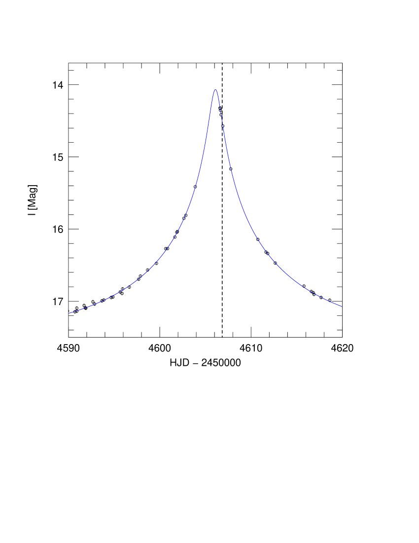
Figure 2: OGLE photometry of the microlensing event. Maximum brightness was estimated to occur on HJD2454606.097 ($\pm 0.004$) i.e., UT2008-05-20.06. The solid line is a theoretical fit to the microlensing event. The vertical dotted line indicates when observations (start of first exposure) were carried out with MIKE (HJD2454606.838).

In May 2008 the OGLE early warning system (Udalski 2003) put out an alert that a new microlensing event, OGLE-2008-BLG-209, was developing and would reach maximum brightness on HJD2454606.097. The faintness of the source star before the microlensing event made it likely for the source star to be a dwarf star in the Bulge, located close to Baade’s window at $(l,\,b)=(1.4,\,-4.0)$ deg (see Fig. 1). Fortunately we had observing time on Magellan II telescope at this time allowing us to obtain a high-resolution spectrum of the object with the MIKE spectrograph (Bernstein et al. 2003). At the time of observation on May 20, 2008 (HJD2454606.838) the event had just passed maximum brightness and had a magnitude of $I\sim 14.5$, about 20 times brighter (approximately 3 magnitudes) than before being microlensed (see Fig. 2). Three 1800 s exposures were obtained using a slit width of 0.7 arcsec, resulting in a spectrum, with continuous wavelength coverage from 3200 Å to 10 000 Å, recorded on two CCDs. With a 0.7 arcsec slit the resolving power is $R\sim 55\,000$ on the blue CCD and $R\sim 47\,000$ on the red CCD. The data were reduced with the Carnegie Observatories MIKE Python pipeline (D. Kelson, private communication) and the final spectrum used in the analysis consists of the three individual spectra co-added and then divided by the blaze function. Typical signal-to-noise ratios are $S/N\sim 20$ per pixel in the spectrum from the blue CCD and $S/N\sim 30$ per pixel in the spectrum from the red CCD (as measured in the continuum of regions free of spectral lines).

2.3 OGLE-2006-BLG-265S, MOA-2006-BLG-099S, and OGLE-2007-BLG-349S

Johnson et al. (2007) presented a detailed abundance analysis of OGLE-2006-BLG-265S. At the time of observation it was magnified by a factor of $\sim 145$ and, by using the HIRES spectrograph on the Keck telescope, they obtained a spectrum of high-resolution ($R\sim 45\,000$) and relatively high signal-to-noise ratio ($S/N\sim 60$ per resolution element).

A year later, Johnson et al. (2008) presented a detailed abundance analysis of MOA-2006-BLG-099S, another microlensed Bulge dwarf star. This object was at the time of observation magnified by a factor of $\sim 110$, and a spectrum was obtained with the MIKE spectrograph on the Magellan II telescope. Compared to OGLE-2006-BLG-265S, the spectrum of MOA-2006-BLG-099S is of lower quality with a resolution of only $R\sim 19\,000$ red-ward of 4800 Å and $S/N\sim 30$ per pixel.

OGLE-2007-BLG-349S, the third dwarf reanalysed here, was observed on September 5, 2007 at the Keck Observatory. Three consecutive spectra, each 1350 s in length, were obtained with HIRES-R at the Keck I telescope in a configuration with coverage from 3900 to 8350 Å, with small gaps between the orders beyond 6650 Å. The slit was 0.86 arcsec wide, giving a spectral resolution of $R\sim 48,000$. The magnifications at the time of the recording of the three spectra were 350, 390, and 450. The signal-to-noise ratio of the resulting summed spectrum is $S/N\sim 30$ per spectral resolution element for wavelengths below 5000 Å and $S/N\sim 90$ for wavelengths above 5500 Å.

Further details about observations and data reductions for these three stars can be found in Johnson et al. (2007, 2008) and Cohen et al. (2008).

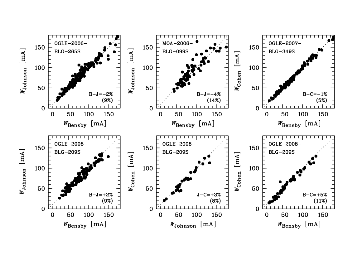
Figure 3: Comparison of equivalent widths measured independently by Bensby (B), Cohen (C) and Johnson (J) for the four stars that have been analysed. Differences and standard deviations (in parentheses) are indicated in the figure. The dotted line in each plot indicates the one-to-one relation.

2.4 Radial velocities

For OGLE-2008-BLG-209S we measure a velocity shift of $-190.1\pm 0.4\,{\rm\,km\,s^{-1}}$ in the spectrum from the blue CCD and $-189.0\pm 0.1\,{\rm\,km\,s^{-1}}$ in the spectrum from the red CCD. As the red spectrum is of higher quality we use this one only for the radial velocity. Adding the heliocentric correction, which at the time of observation was $+15.4\,{\rm\,km\,s^{-1}}$, the heliocentric radial velocity of OGLE-2008-BLG-209S is $-173.6\,{\rm\,km\,s^{-1}}$. The three stars, OGLE-2006-BLG-265S, MOA-2006-BLG-099S, and OGLE-2007-BLG-349S have radial velocities of $+99$, $-154$, and $+113\,{\rm\,km\,s^{-1}}$, respectively (Johnson et al. 2007, 2008; Cohen et al. 2008).

3 Abundance analysis

Stellar parameters and elemental abundances will be determined independently by three of us (T.B., J.J., and J.C.) using different approaches. The different methods will use their own linelists, atomic data, and model stellar atmospheres as used in the various previous studies of Bulge as well as local dwarf stars. As equivalent widths are the fundamental ingredient for all four methods, we will start by checking the agreement between the different measurements for lines that are in common.

3.1 Linelists and equivalent width comparisons

The analysis by Bensby (methods 1 and 2 below) uses the same spectral line list and atomic data as in (Bensby et al. 2003, 2005). However, it has now been expanded by another 50 Fe i lines (see Bensby et al. 2009, in prep.; and Table 2). Equivalent widths were measured by hand using the IRAF task splot. Gaussian line profiles were fitted to the observed lines and in special cases of strong Mg, Ca, Si, and Ba lines, we used Voigt profiles instead to better account for the extended wing profiles of these lines.

The analysis by Johnson (method 3 below) uses a linelist that for most elements was taken from Bensby et al. (2003, 2004). The equivalent widths were measured using SPECTRE (C. Sneden, 2007, private communication). For Ba, synthetic spectra were compared to the observed spectra to determine the abundance. The effect of hyperfine splitting (HFS) in the Ba lines was included and the Ba HFS constants and $\log gf$-values were taken from the sources listed in Johnson et al. (2006).

The analysis by Cohen (method 4 below) uses the linelist given in Cohen et al. (2008). Equivalent widths were measured using an automatic Gaussian fitting routine, after which stronger lines were checked by hand in order to make sure that damping wings were picked up when appropriate. Elements with only a few detected lines were also checked by hand.

Table 1: Comparison of equivalent widths measured by Bensby, Johnson and Cohen. For each element we give the total number of lines that each of the different linelists contain, the average differences (in percent), the 1-sigma spreads, and the number of lines in common (in parentheses).

	OGLE-2008-BLG-209S						MOA-2006-BLG-099S			OGLE-2006-BLG-265S			OGLE-2007-BLG-349S
	Ben	John	Coh	Ben-John	Ben-Coh	John-Coh	Ben	John	Ben-John	Ben	John	Ben-John	Ben	Coh	Ben-Coh
	$N$	$N$	$N$	% $\pm\sigma$ ($N$)	% $\pm\sigma$ ($N$)	% $\pm\sigma$ ($N$)	$N$	$N$	% $\pm\sigma$ ($N$)	$N$	$N$	% $\pm\sigma$ ($N$)	$N$	$N$	% $\pm\sigma$ ($N$)
Total	284	146	109	$+2\pm 9$ (135)	$+5\pm 11$ (55)	$+3\pm 8$ (32)	251	105	$-4\pm 14$ (76)	188	219	$-2\pm 8$ (172)	181	249	$-1\pm 5$ (117)
Fe i	145	72	101	$-1\pm 10$ (61)	$+4\pm 11$ (49)	$+3\pm 8$ (31)	122	35	$-5\pm 11$ (19)	91	98	$-2\pm 8$ (79)	91	135	$-0\pm 3$ (59)
Fe ii	19	2	8	$+4\pm 8$ (2)	$+12\pm 12$ (6)	$+9\pm 0$ (1)	14	4	$-3\pm 9$ (3)	21	9	$-3\pm 14$ (8)	14	11	$-2\pm 8$ (11)

Figure 3 shows comparisons of the equivalent widths as measured by Bensby, Johnson, and Cohen. There is generally a good agreement. For OGLE-2008-BLG-209S Bensby’s measurements are on average 5 % larger than Cohen’s (55 lines in common), and 2 % larger than Johnson’s (135 lines in common), which in turn are 3 % larger than Cohen’s (34 lines in common). For OGLE-2006-BLG-265S the Bensby measurements are just 2 % smaller (172 lines in common) than the measurements by Johnson et al. (2007), and for MOA-2006-BLG-099S the Bensby measurements are 4 % smaller (76 lines in common) than the ones by Johnson et al. (2008). For OGLE-2007-BLG-349S, which has the highest SNR spectrum of the four microlensed stars, the agreement is even better, the Bensby measurements are only 1 % smaller than the measurements by Cohen et al. (2008) (117 lines in common). These differences relate to all equivalent widths from all elements and ions measured. By comparing the equivalent widths of the Fe i and Fe ii lines only, we see that there are significant larger average differences for the Fe ii lines than for the bulk of lines (see Table 1). For instance, for OGLE-2008-BLG-209S the differences in equivalent widths between Bensby’s and Cohen’s measurements of Fe ii lines reach 12 %. How these differences affect the stellar parameters is further investigated in Sect. 3.6.

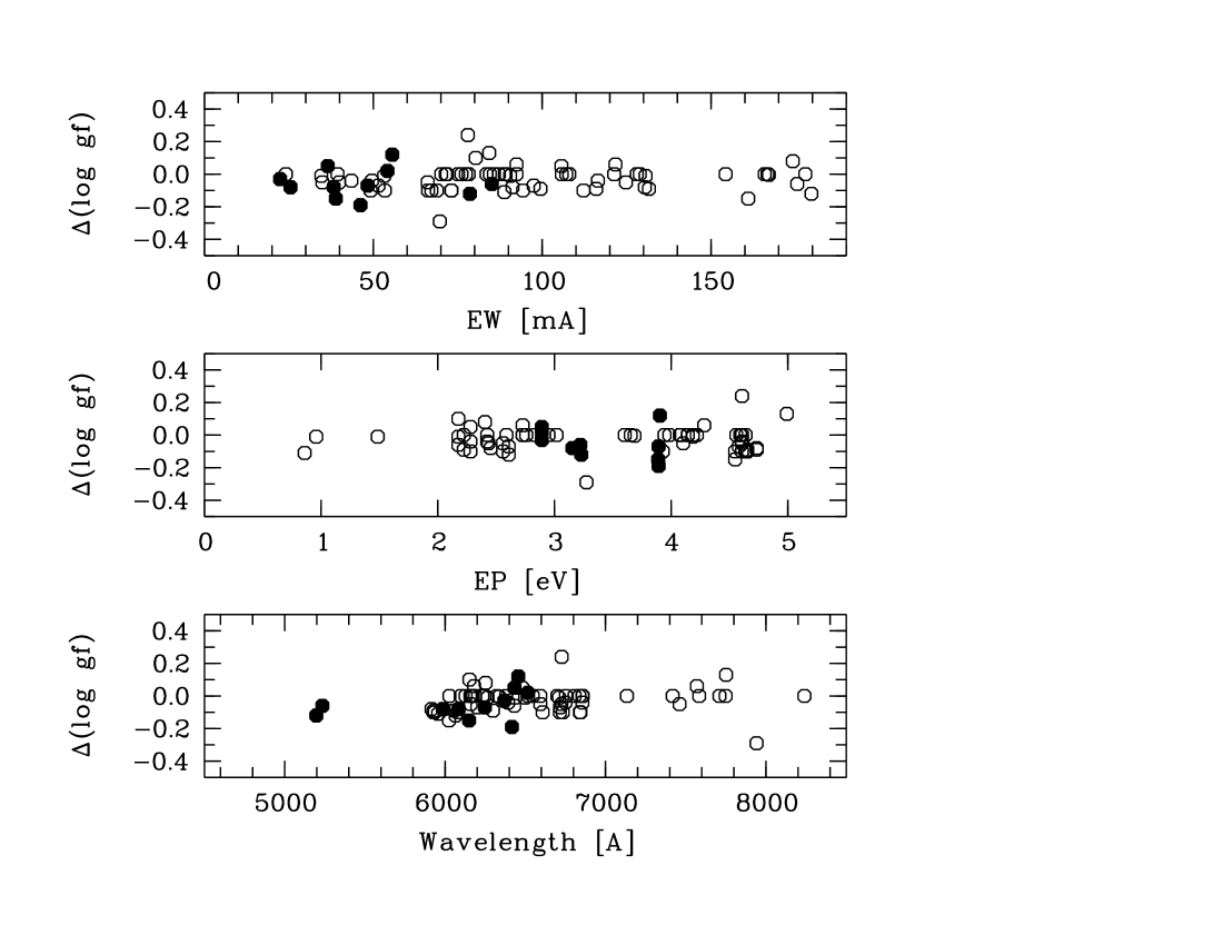
Figure 4: Comparison of Fe i and Fe ii oscillator strengths ($\log gf$) used in methods 1 and 2 (values taken from Bensby et al. 2003, and Bensby et al. 2009, in prep.) and method 4 (values taken from Cohen et al. 2008). The plots show Bensby’s values minus Cohen’s values as a function of line strength (top panel), in this case Cohen’s measurements for OGLE-2007-BLG-349S; lower excitation potential (middle panel); and wavelength (bottom panel). Open and filled circles mark Fe i and Fe ii lines, respectively. On average the Cohen values are $0.03\pm 0.07$ dex larger for the Fe i lines and and $0.05\pm 0.09$ dex larger for the Fe ii lines (i.e. giving lower abundances).

Figure 4 shows a comparison of oscillator strengths ($\log gf$-values) for Fe i and Fe ii lines. Since the Johnson studies largely have adopted the linelists and atomic data as given in Bensby et al. (2003) we only make comparisons between the Bensby and Cohen linelists. The figure shows the differences in the $\log gf$-values as a function of wavelength, as a function of the lower excitation potential of the line, and as a function of the equivalent width. From these plots we see that there are differences present, however with no obvious trends with either excitation potential, line strength, or wavelength. Average differences are $-0.03\pm 0.07$ dex for Fe i lines and $-0.05\pm 0.09$ dex for Fe ii lines, with the values from Cohen linelist being the larger ones. This means that for a given combination of stellar parameters, the average absolute iron abundances by Cohen et al. (2008) will come out $0.03$ dex lower if based on Fe i lines and $0.05$ dex lower if based on Fe ii lines, if the same equivalent widths and model atmospheres are used.

As the tuning of the stellar parameters are based on absolute abundances from Fe i and Fe ii lines (i.e. not normalised to the solar abundances) these differences may have an effect on how the stellar parameters come out from the different methods. This will be investigated further in Sect. 3.6. Note that it is essentially only for the Fe lines that good accuracy of the $\log gf$-values are important. Abundances based on lines from other elements will be normalised to those of the Sun, cancelling, to first order, out any uncertainties in the $\log gf$-values.

Also, the two Fe i lines at 6726 Å and 7941 Å clearly show larger deviations than the other lines (see Fig. 4). In Table 2, where we give abundances for all lines we see that the solar abundance from the $\lambda$6726 line is too low, and from the $\lambda$7941 line it is too high. The normalised abundances from these two lines for the four stars agree however well with the normalised abundances from the other Fe i lines. So, it seems that the $\log gf$ values for these two lines could be significantly off. However, as disregarding the two lines have no effects on the stellar parameters nor the final abundances, we will, for the moment, keep them as they are.

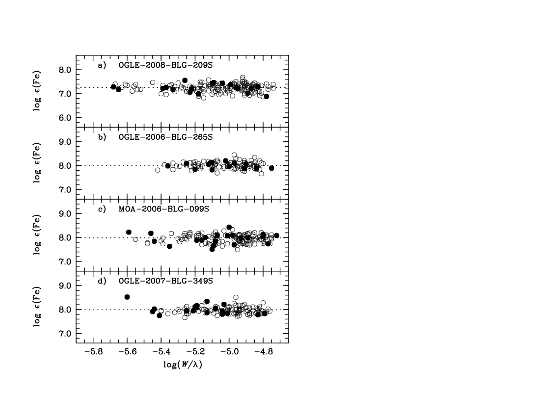
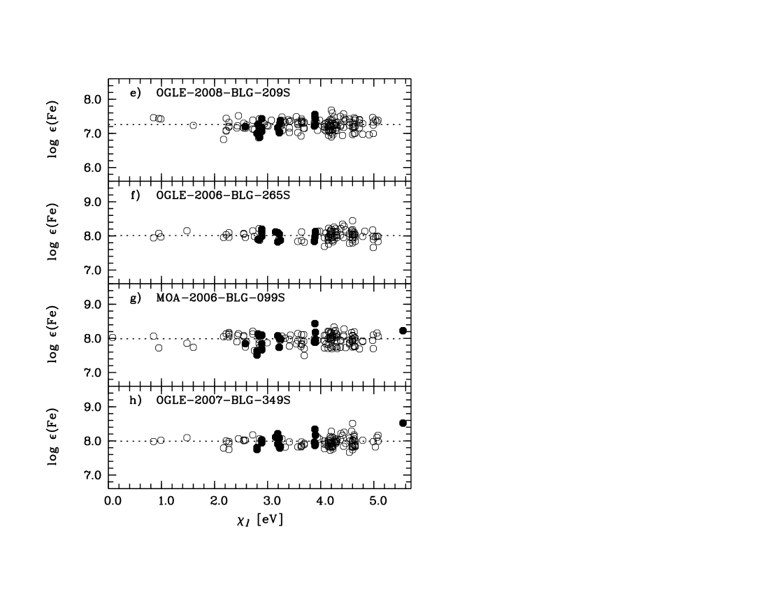
Figure 5: Absolute Fe abundances versus reduced line strength and versus lower excitation potential of the line. Empty circles are abundances from Fe i lines and filled circles from Fe ii lines. The dashed lines are the linear regression to the Fe i abundances.

The Bensby linelist, with measured equivalent widths and calculated elemental abundances for OGLE-2008-BLG-209S, OGLE-2006-BLG-265S, MOA-2006-BLG-099S, and OGLE-2007-BLG-349S is given in Table 2.

3.2 Method 1: Bensby analysis with gravity from ionisation balance

This is a standard method based one-dimensional plane-parallel LTE model stellar atmospheres that were calculated with the Uppsala MARCS code (Gustafsson et al. 1975; Edvardsson et al. 1993; Asplund et al. 1997). Elemental abundances were calculated with the associated suite of programs for abundance analysis and line synthesis (EQWIDTH and SPECTRUM, Edvardsson, Eriksson, & Gustafsson, 2000, private comm.). The resulting stellar parameters and elemental abundances are all based on the equivalent widths measured by T. Bensby. The choice of these MARCS model atmospheres ensures that the results based on this method are fully compatible with our studies of nearby dwarf stars belonging to the Galactic thin and thick discs (Bensby et al. 2003, 2005, and Bensby et al. 2009, in prep.). To find the stellar parameters we use a grid of approximately $12\,000$ MARCS model stellar atmospheres spanning metallicities between $\rm-2.2\leq[Fe/H]\leq+0.7$ in steps of 0.1 dex; surface gravities between $3.2\leq\log g\leq 4.8$ in steps of 0.1 dex, and temperatures between $4500\leq T_{\rm eff}\leq 7000$ K in steps of 100 K (see Bensby et al. 2009, in prep.). The models have chemical compositions scaled relative to the standard solar abundances of Asplund et al. (2005). However, to better reflect the actual composition of the stars, starting at solar metallicity, the models have $\alpha$-enhancements that increase with decreasing metallicity, reaching $[\rm\alpha/Fe]=0.40$ at $\rm[Fe/H]=-1.0$. Below $\rm[Fe/H]=-1.0$ the $\alpha$-enhancement is constant at $[\rm\alpha/Fe]=0.40$, and above the solar metallicity, $\rm[Fe/H]=0$, there is no $\alpha$-enhancement. When calculating abundances the broadening by collisions were taken from Anstee & O’Mara (1995); Barklem & O’Mara (1997, 1998); Barklem et al. (1998, 2000). For lines not included in these works the classical Unsöld broadening was used (see Bensby et al. 2003).

The stellar parameters are determined using the abundances from Fe i and Fe ii lines. The basic concepts of the method are as follows: (1) The effective temperature ($T_{\rm eff}$) is determined by requiring zero slope in the diagram where abundances from the Fe i lines are plotted versus the lower excitation energy of the line ($\chi_{\rm l}$), i.e. excitation equilibrium; (2) The microturbulence parameter ($\xi_{\rm t}$) is determined by requiring zero slope in the diagram where abundances from Fe i lines are plotted versus the measured line strength ($\log(W/\lambda))$; (3) The surface gravity is determined by requiring that the average abundance from the Fe i lines equals the average abundance from Fe ii lines, i.e. ionisation equilibrium. This method was used because we do not know the apparent magnitude nor the distance of the star. All of these balances are coupled and it is not possible to first tune one parameter and then another. All parameters have to be found simultaneously, and after extensive testing we find that an acceptable solution can only be found for one set of parameters for a given star. Final diagnostic plots for $T_{\rm eff}$ and $\xi_{\rm t}$ are shown in Fig. 5. The ionisation balance was deemed good when the average output abundances from the Fe i and Fe ii lines agreed within 0.01 dex. Also, to avoid uncertainties in the stellar parameters arising due to saturation effects in strong lines, only Fe i and Fe ii lines with measured equivalent widths smaller than 90 mÅ were used in the determination of the stellar parameters.

There are indications that abundances from some Fe i lines may be sensitive to departures from LTE which could invalidate our assumption of ionisation balance when determining the surface gravity. However, the predicted correction for a dwarf star at $\rm[Fe/H]=-0.5$ is small, around 0.05 dex (Thévenin & Idiart 1999). Furthermore, in Bensby et al. (2003, 2005) and Bensby et al. (2009, in prep.) we have analysed a total of $\sim 700$ nearby F and G dwarf stars in the Solar neighbourhood, all having accurate distances from the new reduction by van Leeuwen (2007) of the parallaxes from the Hipparcos satellite. The fact that for these $\sim 700$ F and G dwarf stars we do not require ionisation equilibrium, but anyway find a very good agreement between abundances from the two ionisation stages of iron ($\rm[{Fe\textsc{i}}/{Fe\textsc{ii}}]=0.01\pm 0.07$), means that ionisation balance should be a valid option to use for F and G dwarf stars when the distance and/or the apparent magnitude is unknown. Hence, Method 1 and the method for nearby dwarf stars as presented in Bensby et al. (2003, 2005) and Bensby et al. (2009, in prep.), where the distances and magnitudes of the stars are known, should produce results that are fully compatible.

3.3 Method 2: Bensby analysis with gravity based on microlensing assumptions

This method is similar to method 1 and only differs in the way the surface gravity is estimated. Instead of using ionisation balance the surface gravity will be determined using an absolute magnitude estimated from microlensing techniques. As the linelists, equivalent width measurements, model stellar atmospheres, are the same as in method 1, we only describe how the absolute magnitude is estimated.

De-reddened colours and magnitudes of the source can be estimated using standard microlensing techniques (e.g. Yoo et al. 2004). The method for determining the colour does not make any assumption about the absolute reddening, nor about the ratio of selective to total extinction. It only assumes that the reddening to the microlensed source is the same as the reddening to the red clump, and that the red clump has $(V-I)_{0}=1.00$, the same as the local Hipparcos red clump. However, in principle, the Bulge red clump could be different due to different age and composition of the Bulge as compared to the Solar neighbourhood stars. From the spectroscopic temperatures of the three previous Bulge dwarf stars (Johnson et al. 2007, 2008; Cohen et al. 2008) it is found that the mean Bulge clump has $(V-I)_{0}=1.05$. This value is in good agreement with a completely independent estimate based on taking into account the age and differences in composition between the Bulge and the Hipparcos stars (David Bennett, private communication). $(V-I)_{0}=1.05$ for the red clump will be the value used in this study. The absolute de-reddened colour is then derived from the colour offset between the microlensing source and the clump in the instrumental colour-magnitude diagram (CMD). $V$ and $I$ measurements give a colour estimate of $(V-I)_{0}=0.73$ for OGLE-2008=BLG-209S.

The de-reddened apparent magnitude of the source is determined in a similar way, using an assumed de-reddened apparent magnitude of the red clump $(I_{0}=14.32)$ and the offset between the apparent magnitudes of the source and the clump on the instrumental CMD. The instrumental magnitude of the source is determined from the microlensing model. This yields $I_{0}=17.05$ for OGLE-2008-BLG-209S. The absolute magnitude of the source is then determined from assuming that the red clump stars are at the same distance as the source. For OGLE-2008-BLG-209S the estimate for the apparent magnitude is $V_{0}=17.68$, and the absolute magnitude is then $M_{V}=3.26$ (calculated assuming a distance of 8 kpc).

Using this absolute magnitude the stellar parameters are then found in the same way as for method 1, except that ionisation equilibrium is not required.

Table 2: Bensby’s linelist with measured equivalent widths and calculated elemental abundances for OGLE-2008-BLG-209S. Also included are the equivalent widths and elemental abundances measured by Bensby in the solar spectrum and in spectra for OGLE-2006-BLG-265S, MOA-2006-BLG-099S, and OGLE-2007-BLG-349S provided by Cohen and Johnson. For each line we give the $\log gf$ value, lower excitation potential ($\chi_{\rm l}$), measured equivalent widths ($W_{\rm\lambda}$), derived absolute abundance ($\log\epsilon(X)$), abundance normalised to the Sun (on a line-by-line basis) ([$X$/H]). The “flag” for the Sun indicates that a line has not been measured in the solar spectrum and that the abundance given (and used in the normalisation) for that line is the average abundance based on all the other lines, that could be measured in the solar spectrum, of the same species. The table is only available in the online version of the paper and in electronic form at the CDS via anonymous ftp to cdsarc.u-strasbg.fr (130.79.125.5) or via http://cdsweb.u-strasbg.fr/Abstract.html.

					Sun			OGLE-2008-BLG-209			OGLE-2006-BLG-265			MOA-2006-BLG-099			OGLE-2007-BLG-349
Element		Wavelength	$\log gf$	$\chi_{\rm l}$	$W_{\rm\lambda,\odot}$	$\log\epsilon(X)_{\odot}$	flag	$W_{\rm\lambda}$	$\log\epsilon(X)$	[$X$/H]	$W_{\rm\lambda}$	$\log\epsilon(X)$	[$X$/H]	$W_{\rm\lambda}$	$\log\epsilon(X)$	[$X$/H]	$W_{\rm\lambda}$	$\log\epsilon(X)$	[$X$/H]
Al	1	5557.063	-2.21	3.14	10.4	6.44	–	17.1	6.45	0.01	39.9	7.04	0.60	29.4	7.00	0.56	37.9	6.89	0.45
Al	1	6696.023	-1.62	3.14	44.9	6.62	–	47.9	6.45	-0.17	87.8	7.09	0.47	58.8	6.84	0.23	89.5	7.03	0.41
⋮	⋮	⋮	⋮	⋮	⋮	⋮	⋮	⋮	⋮	⋮	⋮	⋮	⋮	⋮	⋮	⋮	⋮	⋮	⋮

3.4 Method 3: Analysis by Johnson

TurboSpectrum (Alvarez & Plez 1998), a 1-dimensional LTE code, was used to derive elemental abundances. The input model stellar atmospheres were interpolated in a grid of the new MARCS 2008 model atmospheres (Gustafsson et al. 2008). These models have chemical compositions scaled relative to the standard solar abundances in Grevesse et al. (2007), but with $\alpha$-enhancements for sub-solar metallicities that are the same as used for the MARCS 1997 models in methods 1 and 2 above (see Sect. 3.2). When calculating elemental abundances the treatment of damping from Barklem et al. (2000) was used.

Effective temperatures and the microturbulence velocities were determined using standard techniques in a similar way to Method 1, including $\log g$ that was determined by demanding ionisation equilibrium. The final parameters adopted for OGLE-2008-BLG-209S were $T_{\rm eff}=5250$ K, $\log g=3.5$, metallicity $\rm[Fe/H]=-0.40$, and $\xi_{\rm t}=1.4\,{\rm\,km\,s^{-1}}$.

Further details of the method can be found in Johnson et al. (2007, 2008). It should be noted that an attempt to measure the effective temperature from the Balmer H$\alpha$ line, as was done for MOA-2006-BLG-099S in Johnson et al. (2008), was made, but the cool temperature of OGLE-2008-BLG-209S meant that no accurate $T_{\rm eff}$ could be derived this way.

3.5 Method 4: Analysis by Cohen

This method is also based on standard LTE assumptions, using a grid of solar scaled ATLAS9 model stellar atmospheres from Castelli & Kurucz (2003). In the analysis for OGLE-2008-BLG-209S, only lines with wavelengths longer than 5400 Å were selected due to the low $S/N$ in the crowded blue parts of the spectrum. Also, the stronger lines in these high gravity dwarf stars with their extended damping wings, which are difficult to measure in crowded spectra of only moderate $S/N$, are rejected. As in methods 1-3, damping constants from Barklem et al. (2000) were used when available. Abundances were calculated with the MOOG 2002 package (Sneden 1973).

The effective temperature is determined by requiring excitation equilibrium for the set of Fe i lines with measured equivalent widths less than 130 mÅ. The microturbulence velocity ($\xi_{\rm t}$) is solved for in the standard way. As a first pass, models with surface gravity of $\log g=4.5$, and with solar metallicity are used. The [Fe/H] value is then determined from the set of Fe i lines with lower excitation potential greater than 4.0 eV and equivalent widths less than 130 mÅ using that choice for $T_{\rm eff}$. The calculation is repeated with different metallicity models if the output of the first pass differs significantly from that of the input model atmosphere. The surface gravity then follows by demanding ionisation equilibrium between Fe i and Fe ii. The rationale behind this method is further described in Cohen et al. (2009, in preparation), and additional details can be found in Cohen et al. (2008).

3.6 Comparisons of stellar parameters from methods 1–4

Below we present the stellar parameters for the four stars and compare them to the ones found by the different methods and by Johnson et al. (2007, 2008) and Cohen et al. (2008). All values are given in Table 3.

Table 3: Stellar parameters as determined from the different methods.

Object	$(V-I)_{0}$	$I_{0}$	$V_{0}$	$M_{\rm V}$	$d$	$T_{\rm eff}$	$\log g$	$\xi_{\rm t}$	Mass	$\log\epsilon({\rm Fe})$		[Fe/H]	Age
	$\rm[mag]$	$\rm[mag]$	$\rm[mag]$	$\rm[mag]$	$\rm[kpc]$	$\rm[K]$	$\rm[cgs]$	$\rm[{\rm\,km\,s^{-1}}]$	$\rm[M_{\odot}]$	Fe i	Fe ii		$\rm[Gyr]$
OGLE-2008-BLG-209S	–	–	18.35	3.83	8.0	5243	3.82	1.01	1.02	7.24	7.24	$-0.33$	8.5	Method 1
”	0.73	17.05	17.68	3.16	8.0	5307	3.69	1.13	1.31	7.26	7.12	$-0.31$	3.8	Method 2
”						5250	3.60	1.40		7.04	7.04	$-0.42$		Method 3
”						5325	3.60	1.30		7.16	7.16	$-0.32$		Method 4
OGLE-2006-BLG-265S	–	–	19.10	4.58	8.0	5486	4.24	1.17	1.05	8.02	8.01	$0.44$	7.5	Method 1
”	0.68	18.11	18.69	4.17	8.0	5526	4.11	1.25	1.10	8.02	7.91	$0.44$	7.0	Method 2
”				4.30		5650	4.40	1.20		8.05	8.07	$0.56$		Johnson et al. (2007)
MOA-2006-BLG-099S	–	–	19.35	4.83	8.0	5741	4.47	0.84	1.12	7.96	7.95	$0.39$	*	Method 1
”	0.74	18.17	18.81	4.29	8.0	5852	4.32	1.03	1.18	7.99	7.81	$0.42$	2.8	Method 2
”				4.50		5800	4.40	1.50				$0.36$		Johnson et al. (2008)
OGLE-2007-BLG-349S	–	–	19.35	4.83	8.0	5229	4.18	0.78	0.94	7.96	7.95	$0.41$	13.0	Method 1
”	0.78	18.72	19.40	4.88	8.0	5210	4.18	0.76	0.93	7.96	7.96	$0.40$	13.7	Method 2
”						5480	4.50	1.00		8.02		$0.51$		Cohen et al. (2008)

Table 4: Elemental abundance ratios, $[X/{\rm H}]$, as determined from the different methods.

Object	O i	Na i	Mg i	Al i	Si i	Ca i	Ti i	Ti ii	Cr i	Cr ii	Ni i	Fe i	Fe ii	Zn i	Y ii	Ba ii
OGLE-2008-BLG-209S	$0.06$	$-0.18$	$0.01$	$-0.04$	$-0.13$	$-0.15$	$-0.14$	$0.03$	$-0.29$	$-0.27$	$-0.28$	$-0.33$	$-0.28$	$-0.31$	$-0.45$	$-0.30$	Method 1
”	$-0.07$	$-0.12$	$0.09$	0.00	$-0.15$	$-0.08$	$-0.09$	$-0.05$	$-0.23$	$-0.37$	$-0.27$	$-0.31$	$-0.40$	$-0.37$	$-0.54$	$-0.32$	Method 2
”	$-0.08$	$-0.28$	$-0.14$	$-0.09$	$-0.25$	$-0.30$	$-0.26$	$-0.04$	$-0.33$	–	$-0.36$	$-0.42$	$-0.44$	$-0.36$	$-0.77$		Method 3
”												$-0.32$					Method 4
OGLE-2006-BLG-265S	0.28	0.58	0.56	0.52	0.49	0.37	0.42	0.34	0.45	0.26	0.49	0.44	0.43	0.32	0.52	0.29	Method 1
”	0.18	0.64	0.63	0.55	0.47	0.43	0.45	0.27	0.47	0.18	0.48	0.44	0.33	0.30	0.45	0.25	Method 2
”	$-0.03$	0.62	0.48	0.81	0.48	0.33	0.46		0.64		0.62	0.55	0.57			0.53	Johnson et al. (2007)
MOA-2006-BLG-099S	0.37	0.46	0.45	0.42	0.37	0.31	0.36	0.45	0.25	0.28	0.39	0.39	0.41	0.47	0.42	0.37	Method 1
”	0.22	0.56	0.56	0.48	0.38	0.42	0.43	0.36	0.32	0.16	0.42	0.42	0.28	0.44	0.31	0.36	Method 2
”	0.20	0.45	0.52	0.47	0.42	0.25	0.31	0.14			0.38	0.36	0.18	0.08		$-0.25$	Johnson et al. (2008)
OGLE-2007-BLG-349S	$0.34$	$0.55$	$0.43$	0.49	$0.47$	$0.31$	$0.43$	$0.41$	$0.40$	$0.41$	$0.48$	$0.41$	$0.42$	$0.49$	$0.26$	$0.19$	Method 1
”	$0.37$	$0.54$	$0.42$	0.48	$0.48$	$0.30$	$0.41$	$0.42$	$0.39$	$0.42$	$0.48$	$0.40$	$0.44$	$0.50$	$0.27$	$0.19$	Method 2
”	$0.14$	$0.77$	$0.59$	0.49	$0.47$	$0.55$	$0.53$	$0.67$	$0.53$		$0.67$	$0.51$	$0.43$	$0.42$		$0.38$	Cohen et al. (2008)

OGLE-2008-BLG-209S:

The derived stellar parameters, $\log g=3.6$ to 3.8, and $T_{\rm eff}=5200$ to 5300 K, are consistent with OGLE-2008-BLG-209S being a subgiant star which also can be seen in Fig. 8. Furthermore, we find that OGLE-2008-BLG-209S has a sub-solar metallicity of $\rm[Fe/H]\approx-0.33$ (ranging between $\rm[Fe/H]=-0.42$ and $\rm[Fe/H]=-0.32$ for the different methods). This relatively low metallicity is in stark contrast to the previous three Bulge dwarf stars that were all determined to have highly super-solar metallicities: two with $\rm[Fe/H]>0.5$ (Johnson et al. 2007; Cohen et al. 2008), and one with $\rm[Fe/H]>0.3$ (Johnson et al. 2008). From methods 1 and 2 we find an age for OGLE-2008-BLG-209S ranging between 4-8 Gyr (see Fig. 8).

OGLE-2006-BLG-265S:

The effective temperature from the different methods and from Johnson et al. (2007) agree quite well and range between 5500 to 5650 K. Also the surface gravity is well constrained between $\log g=4.1$ to 4.4, values that are typical for dwarf stars. Using methods 1 and 2 we find that OGLE-2006-BLG-265S is a very metal-rich star at $\rm[Fe/H]=0.44$. It is however 0.12 dex lower than in Johnson et al. (2007) who finds $\rm[Fe/H]=0.56$. From methods 1 and 2 we find that OGLE-2006-BLG-265S has an age of approximately 7 Gyr (see Fig. 8). From Fig. 8 we see that OGLE-2006-BLG-265S is a dwarf star close to the main sequence turn-off.

MOA-2006-BLG-099S:

Methods 1 and 2 give $T_{\rm eff}=5741$ to 5852 K, $\log g=4.32$ to 4.47, and $\rm[Fe/H]=0.39$ to 0.42, which are values that are very similar to the results by Johnson et al. (2008) that found $T_{\rm eff}=5800$ K and $\rm[Fe/H]=0.36$. While Johnson et al. (2008) used the microlensing technique to estimate $M_{\rm V}$ (and thus $\log g$), they determined the effective temperature from profile fitting of the wings of the H$\alpha$ and H$\beta$ Balmer lines. Since MOA-2006-BLG-099S falls just outside the limits of the isochrones we can only give an upper limit to its age, which should be approximately 3 Gyr (see Fig. 8). Given the stellar parameters and the position in the $M_{\rm V}$-$T_{\rm eff}$ diagram, it is clear that MOA-2006-BLG-099S is a main sequence dwarf star.

OGLE-2007-BLG-349S:

The stellar parameters based on methods 1 and 2 are very similar: $T_{\rm eff}\approx 5220$ K and $\rm[Fe/H]\approx 0.40$. These results are lower than the ones found by Cohen et al. (2008), $T_{\rm eff}$ by $\sim 260$ K and [Fe/H] by $\sim 0.1$ dex. Given the uncertainties claimed by Cohen et al. (2008) of 100 K in $T_{\rm eff}$ and $\sim 0.1$ dex in [Fe/H], and the uncertainties for methods 1 and 2 as listed in Sect. 5, we see that the metallicities are compatible and also the temperatures, but just barely. We find that OGLE-2007-BLG-349S is a dwarf star close to the main sequence turn-off, and that it has a high age of approximately 13 Gyr (see Fig. 8).

In summary,

the differences we find in the stellar parameters among the groups (and methods), with the possible exception of OGLE-2007-BLG-349S, are easily within the error bars (see Sect. 5).

3.7 Inconsistencies

Equivalent width measurements and $\log gf$-values:

For OGLE-2008-BLG-209S, method 3 gives a $T_{\rm eff}$ similar to methods 1 and 2 but a lower metallicity: 0.2 dex in absolute values and 0.1 dex when normalised to the Sun. The decrease in the difference when normalising to the Sun can be explained as a result of the lower Solar abundances that method 3 produces compared to methods 1 and 2 (see Sect. 4 and Fig. 6). The difference of 0.2 dex in the absolute Fe abundances can be explained by difference of 0.2 dex in $\log g$ and 0.4 ${\rm\,km\,s^{-1}}$ in $\xi_{\rm t}$. In Bensby et al. (2003, 2005) where we in detail investigated the effects of uncertainties in these parameters we see that the above differences in $\xi_{\rm t}$ and $\log g$ would result in a changes of $\sim 0.10-0.15$ dex and $\sim 0.03$ dex, respectively, in the output Fe abundance. Therefore it is clear that it is mainly the microturbulence parameter that is to blame for the different absolute Fe abundances between methods 1 and 3. In Sect. 4 we also show that the output abundances from methods 1 and 3 are very similar if the input equivalent widths are similar and the model stellar parameters are the same. Hence, there are no problems with the model stellar atmospheres (MARCS 1997 versus MARCS 2008), nor the different abundance programs (EQWIDTH versus TurboSpectrum), that are used by methods 1 and 3 in the abundance analysis.

Method 4 gives a higher $T_{\rm eff}$ for OGLE-2008-BLG-209S than methods 1, 2, and 3, and a similar metallicity. As shown in Sect. 3.1 there are significant differences between the Fe i and Fe ii equivalent widths as measured by Bensby and Cohen. The Bensby measurements are 4 % and 12 % larger for Fe i and Fe ii lines, respectively, and can possibly affect the accuracy of the ionisation balance that are used in finding the stellar parameters. To investigate if this could explain the differences in the stellar parameters between methods 1 and 4 we divide the Fe i and Fe ii equivalent widths of Bensby by 1.04 and 1.12, respectively, and redo the determination of the stellar parameters. The effect is a slightly lower effective temperature, 5214 K, from method 1 and does not resolve the problem with the different effective temperatures between methods 1 and 4. However, they only differ by 80 K, which is well within the uncertainties.

In Sect. 3.1 we also found differences in the $\log gf$-values for the Fe i and Fe ii lines between the Bensby and Cohen linelists. Average differences are $-0.03\pm 0.07$ dex for Fe i lines and $-0.05\pm 0.09$ dex for Fe ii lines, with the values from Cohen et al. (2008) being the larger ones. In methods 1 and 2 the abundances from Fe i and Fe ii lines have been used in their absolute form, i.e. they have not been normalised to the Sun, when determining the stellar parameters. Therefore, if the different methods/studies have different $\log gf$-values for the Fe i and Fe ii lines it may have an impact on the stellar parameters. Applying similar corrections to the Fe i and Fe ii $\log gf$-values of the Bensby linelist, as was done above to the Bensby equivalent widths, and redoing the analysis have essentially no effect on the derived parameters.

Furthermore, the recent study by Melendez & Barbuy (2009) claims that there might be problems with the Fe ii $\log gf$-values of Raassen & Uylings (1998) that were adopted by Bensby et al. (2003) and that we use in methods 1 and 2. According to Melendez & Barbuy (2009) these $\log gf$-values are both inaccurate and imprecise. We therefore check our stellar parameters for OGLE-2008-BLG-209S using the revised Fe ii $\log gf$-values by Melendez & Barbuy (2009) and we find slightly different values for the stellar parameters: $T_{\rm eff}=5197$ K, $\log g=3.88$, and $\xi_{\rm t}=0.93$. The age of the star also becomes higher, $12.5\pm 6$ Gyr compared to $8.5\pm 6$ Gyr. Apart from the age difference, these changes are really marginal. Therefore, and as about half the $\log gf$-values by Melendez & Barbuy (2009) are based on an inverse solar analysis (which most likely is the cause for the claimed abundance spread decrease by Melendez & Barbuy 2009), we will keep the theoretical values by Raassen & Uylings (1998). We will then have a single source for our $\log gf$-values, and will also be independent on the methods Melendez & Barbuy (2009) use to measure equivalent widths for these lines, and to their choice of model stellar atmospheres used in the inverse solar analysis.

Colours and temperatures:

From the calibration by Alonso et al. (1996) we check what temperature we should expect given the inferred colour of OGLE-2008-BLG-209S. The Alonso calibration is however in the Johnson system only, so we convert the Johnson-Cousin colour of OGLE-2008-BLG-209S using the relation by Fernie (1983), giving $(V-I)_{J}=0.924$. Applying Eq. (6) in Alonso et al. (1996) we then get a temperature of 5564 K. And what colour would be predicted for this star at T=5250? Using the same equations (in reverse) we get a Johnson-Cousin colour $(V-I)_{0}=0.83$. Double-checking with the colour-$T_{\rm eff}$ calibration of Ramírez & Meléndez (2005) we find that this star should have an intrinsic Johnson-Cousin $(V-I)_{0}\approx 0.82$ if its temperature is about 5250. Hence it seems that all is fine and the temperatures we derive should be good.

However, an intrinsic colour $(V-I)_{0}\approx 0.82$ means that there is an inconsistency in method 2, because $T_{\rm eff}$ is adopted in disagreement of this colour (0.73 compared to 0.82). This could indicate that the reddening perhaps is wrong.

But, is this discrepancy possible? In principle yes. We do have an example of a source (OGLE-2008-BLG-513S) that has 0.3 mag less extinction than the clump. So 0.1 mag is not unheard of. Nevertheless, this discrepancy is still bigger than what has been seen for the other three dwarf stars. Anyway, given the estimated uncertainties in $T_{\rm eff}$ (see Sect. 5) it seems that an effective temperature of 5243 K is not unreasonable for OGLE-2008-BLG-209S.

4 Solar analysis

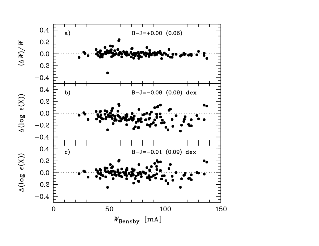
Figure 6: Differences in measured equivalent widths and elemental abundances for the Sun for the Bensby (B) and Johnson (J) analyses of the Ganymede solar spectrum. a) shows the On average the Bensby equivalent widths are $0.4\pm 10$ % larger than Johnson’s (see plot a), and the corresponding Bensby abundances are on average $0.077\pm 0.095$ dex lower than Johnson’s (see plot b). Plot c) then shows the differences when the Bensby abundances are computed using exactly the same stellar parameters as used by Johnson (see discussion in text). The differences then decrease to less than 0.01 dex. Differences and standard deviations (in parentheses) are indicated in the figures and are based on 128 spectral lines that Bensby and Johnson have in common.

For methods 1 and 2 a solar analysis was performed on a spectrum of Jupiter’s moon Ganymede that was obtained in March 2007 with the MIKE spectrograph using the same instrument settings as for the observations of OGLE-2008-BLG-209S. Analysing the solar spectrum in a similar way (as we know the absolute magnitude of the Sun we do not require ionisation equilibrium) as for methods 1 and 2, we derive $T_{\rm eff}=5790$ K, $\log g=4.45$, $\xi_{\rm t}=1.04\,{\rm\,km\,s^{-1}}$, and $\log\,\epsilon({\rm Fe})=7.56$ for the Sun. The final elemental abundances based on methods 1 and 2, will be normalised to those of the Sun from this analysis. The normalisation will be done on a line-by-line basis, and then averaged for each element, making the results strictly differential to the Sun. This way of normalising the abundances neutralises uncertainties and errors in the $\log gf$-values. It should be noted that when a line in the Solar spectrum could not be measured, or, in the case of Fe lines, the line strength exceeded 90 mÅ, the average abundance from all the other lines of the same species were used for the solar abundance of that line. These cases are marked by ”flag=1” in Table 2.

In Table 5 we give the average solar abundances for each species as derived by Bensby from the MIKE Ganymede spectrum. For comparison purposes we also give the standard Solar abundances as given by Asplund et al. (2005) and Grevesse et al. (2007). Generally our Solar abundances agree within 0.1 dex of the standard ones, with O and Ba being the exceptions. The differences, all though they are small, illustrates the importance of doing a strictly differential analysis toward the Sun, deriving your own Solar abundances instead of adopting the tabulated ones.

For method 3, a solar analysis was performed using the same spectrum of Ganymede as was used for methods 1 and 2. The line list and line parameters were the same, and a model stellar atmosphere for the Sun was interpolated in the same grid of model stellar atmospheres as was used for OGLE-2008-BLG-209S, using $T_{\rm eff}=5770$, $\log g=4.44$, $\rm[Fe/H]=0$ ($\log\,\epsilon({\rm Fe})=7.45$), and $\xi_{\rm t}=1.1\,{\rm\,km\,s^{-1}}$.

For method 4, the same set of lines as used for OGLE-2008-BLG-209S were analysed in the Solar spectrum by Wallace et al. (1998). These were then use to determine [X/H] for each species for OGLE-2008-BLG-209S.

As the same Ganymede spectrum was used by both Bensby and Johnson to determine the Solar elemental abundances we show in Figure 6a a comparison of measured equivalent widths and absolute elemental abundances for 128 spectral lines in common. The equivalent width measurements are in good agreement and differs by only 0.5%, with the measurements by Bensby being the slightly larger ones. Surprisingly, this good agreement in the equivalent widths is not reflected in the derived elemental abundances for the Sun. On average the abundances from Bensby’s analysis are 0.08 dex lower than the abundances from Johnson’s analysis (see Fig. 6b). This is puzzling, but it turns out that the solar models used by Bensby and Johnson differ. While Johnson used a MARCS model with $\log\,\epsilon({\rm Fe})=7.45$, Bensby used a MARCS model with $\log\,\epsilon({\rm Fe})=7.56$, and of course the values for the microturbulence parameter also differed slightly. So, redoing the Bensby solar abundances, using exactly the same set of model stellar parameters as used by Johnson, the differences in the solar abundances become less than 0.01 dex (see Fig. 6c). This also explains why the differences between methods 1 and 3 in the Fe abundances are different depending on if comparisons are made between absolute abundances or normalised abundances (see Table 3). As we are primarily interested in comparing stars with each other it is []-notation that is relevant here and it is encouraging to see how well the different methods do reproduce the results (once any differences in the methodology are fully accounted for). This is perhaps not surprising but worth noting and serves as a reminder that if one attempts to combine data from different studies then careful normalisation is a must.

Equivalent widths and absolute elemental abundances (also for the Sun) and normalised abundances are given for individual lines are given in Table 2. Average elemental abundance ratios are given in Table 4. Absolute and normalised abundances from the Fe i and Fe ii lines are also given in Table 3.

Table 5: Our solar abundances based on observations of Jupiter’s moon Ganymede. Last column give the standard Solar photospheric abundances given by Asplund et al. (2005).

Ion	$\log\epsilon(X)_{\odot}$	$N$	A2005
Fe i	$7.57\pm 0.08$	148	7.45
Fe ii	$7.52\pm 0.13$	17	7.45
O i	$8.86\pm 0.02$	3	8.66
Na i	$6.29\pm 0.08$	4	6.17
Mg i	$7.62\pm 0.08$	5	7.53
Al i	$6.48\pm 0.07$	7	6.37
Si i	$7.60\pm 0.07$	27	7.51
Ca i	$6.32\pm 0.11$	19	6.31
Ti i	$4.93\pm 0.11$	22	4.90
Ti ii	$4.90\pm 0.17$	14	4.90
Cr i	$5.55\pm 0.06$	6	5.64
Cr ii	$5.69\pm 0.04$	5	5.64
Ni i	$6.22\pm 0.07$	42	6.23
Zn i	$4.60\pm 0.08$	3	4.60
Y ii	$2.12\pm 0.11$	4	2.21
Ba ii	$2.42\pm 0.07$	4	2.17

5 Errors

5.1 Random errors in stellar parameters

We are performing standard LTE abundance analyses and the associated errors and uncertainties for the stellar parameters should be of standard nature. Methods 1 and 2 are similar to the analysis carried out in Bensby et al. (2003, 2005) where errors of 80 K in $T_{\rm eff}$ and 0.1 dex in $\log g$ are quoted. The line-to-line scatter in those studies for [Fe/H] are of the order 0.08 dex. For OGLE-2008-BLG-209S the standard deviation of the mean abundance in the Fe i abundances are about double that, $\rm\sigma[Fe/H]=0.14$ (see Table 6), which most likely is an effect of the lower quality of the spectrum as compared to the spectra used in Bensby et al. (2003, 2005) that had $S/N\gtrsim 200$. Therefore we estimate that the uncertainties in $T_{\rm eff}$ and $\log g$ should be higher for OGLE-2008-BLG-209S. A conservative estimate is 0.2 dex in $\log g$ and 200 K in $T_{\rm eff}$. The same numbers should hold for OGLE-2006-BLG-265S and MOA-2006-BLG-099S that have errors in the Fe i abundances comparable to OGLE-2008-BLG-209S (see Table 6). The spectrum of OGLE-2007-BLG-349S is however of significantly higher quality than the others, which also is reflected in the lower Fe i standard deviation around the mean abundance, 0.10 dex (see Table 6). Hence, for OGLE-2007-BLG-349S we estimate that the errors in $T_{\rm eff}$, $\log g$ are of the order 150 K and 0.15 dex, respectively. The magnitudes of these errors are in line with the values given by Johnson et al. (2007, 2008) and Cohen et al. (2008) for OGLE-2006-BLG-265S, MOA-2006-BLG-099S, and OGLE-2007-BLG-349S.

In the last column of Table 6 we list by how much the [$X$/Fe] ratios are affected by these uncertainties in the stellar parameters. The values are taken as double the values as listed in Bensby et al. (2005) and Bensby et al. (2004) (for [O/Fe]) where we investigated this in detail (see discussion above).

5.2 Elemental abundances and the robustness of abundance ratios

We find that the $\rm[X/Fe]$ ratios generally agree well between the different methods/studies, and it is essentially only oxygen, zinc, yttrium, and barium that show any real discrepancies for one or two stars. The big difference in $\rm[O/Fe]$ that can be seen compared to Johnson et al. (2007) for OGLE-2006-BLG-265S is clearly an effect of the almost 200 K difference in effective temperature.

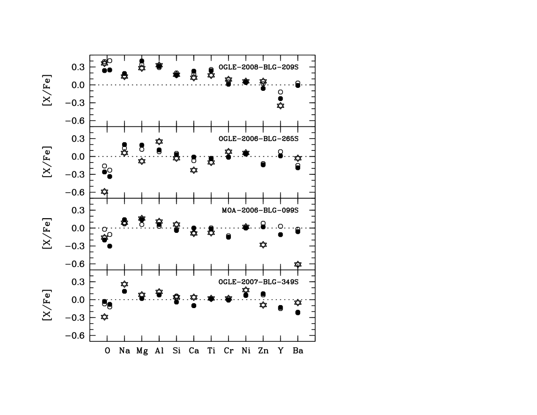
Figure 7: Comparisons of derived $\rm[X/Fe]$ ratios for method 1 (open circles), method 2 (filled circles), and from Johnson et al. (2007, 2008) and Cohen et al. (2008) (stars). F or OGLE-2008-BLG-209S the stars show the values from method 3. For oxygen two values are given side by side: on the left hand side the LTE value as it comes of the analysis, and on the right hand side the NLTE value corrected by the empirical NLTE correction formula from Bensby et al. (2004).

The Ba abundances from Johnson et al. (2007, 2008) are based on line synthesis, and hence the equivalent widths can not be directly compared. However, except for MOA-2006-BLG-099S, where the Johnson et al. (2008) [Ba/Fe] ratio is extremely low, the agreement is good. The low value of MOA-2006-BLG-099S is also not recognised in OGLE-2006-BLG-265S, a similarly metal-rich star. As mentioned in Johnson et al. (2008) the reason for the low [Ba/Fe] value of MOA-2006-BLG-099S was the high value they measured in the Sun. The good agreement for the other stars between Ba as derived by line synthesis and through equivalent width measurement analysis illustrates the point raised by Bensby et al. (2005) that because the dominant isotopes for Ba are the even isotopes, which do not have hyperfine structure, the inclusion of HFS does not substantially change the abundances. Furthermore, the line synthesis of the Ba ii line at 6141 Å done by Johnson in method 3 for OGLE-2008-BLG-209S included an Fe i line that blends with the feature. However, this line contributes very little to the line profile. A synthesis of the line showed that the equivalent width increased from 127.9 nm to 132.7 nm if the Fe i line was included. Therefore, using the equivalent width and assuming that it is all Ba leads to a very small change in the Ba abundance.

6 Bulge membership for OGLE-2008-BLG-209S

Bulge microlensing sources tend to be slightly biased to be more distant than the mean distance to the Bulge (“the Bulge clump”), see e.g. Kane & Sahu (2006). The lens must obviously be in front of the source, so if the lens is in the Bulge (which most are), the source must be drawn from the Bulge stars behind it, so on average more distant than the Bulge centre. In fact, the bias is stronger than that because the probability of lensing goes basically as $\sqrt{(d_{source}-d_{lens})}$ for lenses and source in the Bulge. For disc lenses (the minority) there is no significant bias. This bias would tend to make the source more luminous than the microlens-model based estimate based on assuming it is at the same distance as the red clump. This goes in the opposite direction of the difference between the spectroscopic and microlens determinations of $M_{\rm V}$.

Based on our spectroscopic parameters from method 3, $T_{\rm eff}=5250$ and $\log g=3.6$, we use the Y²-isochrones at $Z=0.007$ to estimate an $M_{\rm I}$ of 2.5. Combined with the $I_{0}=17.05$ microlensing estimate, we derive a distance to OGLE-2008-BLG-209S of 8 kpc. Now, if we take $M_{\rm V}=3.83$ from Table 3, (method 1) and $V_{\rm 0}=17.68$ (microlensing estimate from method 2), the distance comes out to 6 kpc. The difference is probably due to the higher gravity (i.e., fainter absolute magnitude). Since the errors on the gravity are not insignificant (between the small number of Fe ii lines and the correlation between temperature and gravity, not to mention systematic uncertainties between isochrone and spectroscopic determinations), there are large errors attached to both these distances.

However, the high heliocentric radial velocity of OGLE-2008-BLG-209S (see Sect. 2.4) demonstrates that it is likely to be in the Bulge, and the relatively high radial velocities of the other three dwarf stars also strongly suggest Bulge membership. This high velocity dispersion of our four stars is also in agreement with what is seen in large samples of giant stars in the Bulge (e.g. Sadler et al. 1996; Zoccali et al. 2008).

In conclusion, based on the radial velocity, probability of microlensing, and small distance from the Galactic plane, we expect this star to be in the Bulge. This is consistent with the range of distances derived from spectroscopic parameters and isochrones.

Table 6: Final elemental abundance ratios, $[X/{\rm Fe}]$, based on method 1. For each abundance ratio we also give the standard deviation of the mean abundance (added in quadrature for the two elements used to construct the abundance ratio), and the number of lines used. These are the values used in subsequent abundance plots. The last column gives an estimate how the abundance ratios are affected by random errors in the stellar parameters. The adopted uncertainties for the Bulge dwarf stars are two times the values as given in Bensby et al. (2005) and Bensby et al. (2004).

	BLG-209S	BLG-265S	BLG-099S	BLG-349S	$\langle\sigma_{\rm rand}\rangle$
[Fe/H]	$-0.33$	0.44	0.39	0.41	0.12
	0.14	0.12	0.15	0.10
	146	92	119	103
[O/Fe]	0.39	$-0.16$	$-0.02$	$-0.07$	0.24
	0.17	0.13	0.15	0.12
	3	3	3	3
[Na/Fe]	0.15	0.14	0.07	0.14	0.06
	0.16	0.14	0.17	0.16
	4	4	4	4
[Mg/Fe]	0.34	0.12	0.06	0.02	0.12
	0.14	0.17	0.17	0.12
	5	2	4	3
[Al/Fe]	0.29	0.08	0.03	0.08	0.10
	0.17	0.18	0.17	0.15
	7	3	4	3
[Si/Fe]	0.20	0.05	$-0.02$	0.06	0.10
	0.18	0.19	0.20	0.14
	27	23	25	23
[Ca/Fe]	0.18	$-0.07$	$-0.08$	$-0.10$	0.06
	0.20	0.17	0.19	0.14
	19	16	18	18
[Ti/Fe]	0.26	$-0.04$	0.00	0.01	0.10
	0.22	0.15	0.23	0.17
	36	13	30	24
[Cr/Fe]	0.05	$-0.01$	$-0.13$	0.00	0.10
	0.20	0.13	0.19	0.12
	10	8	12	7
[Ni/Fe]	0.05	0.05	0.00	0.07	0.04
	0.23	0.18	0.22	0.14
	40	30	37	39
[Zn/Fe]	0.02	$-0.12$	0.08	0.08	0.12
	0.34	0.58	0.20	0.18
	3	2	3	3
[Y/Fe]	$-0.12$	0.08	0.03	$-0.15$	0.16
	0.18	0.14	0.38	0.16
	4	2	5	5
[Ba/Fe]	0.03	$-0.15$	$-0.02$	$-0.22$	0.12
	0.16	0.17	0.17	0.17
	4	3	4	4

7 Stellar age and stellar mass

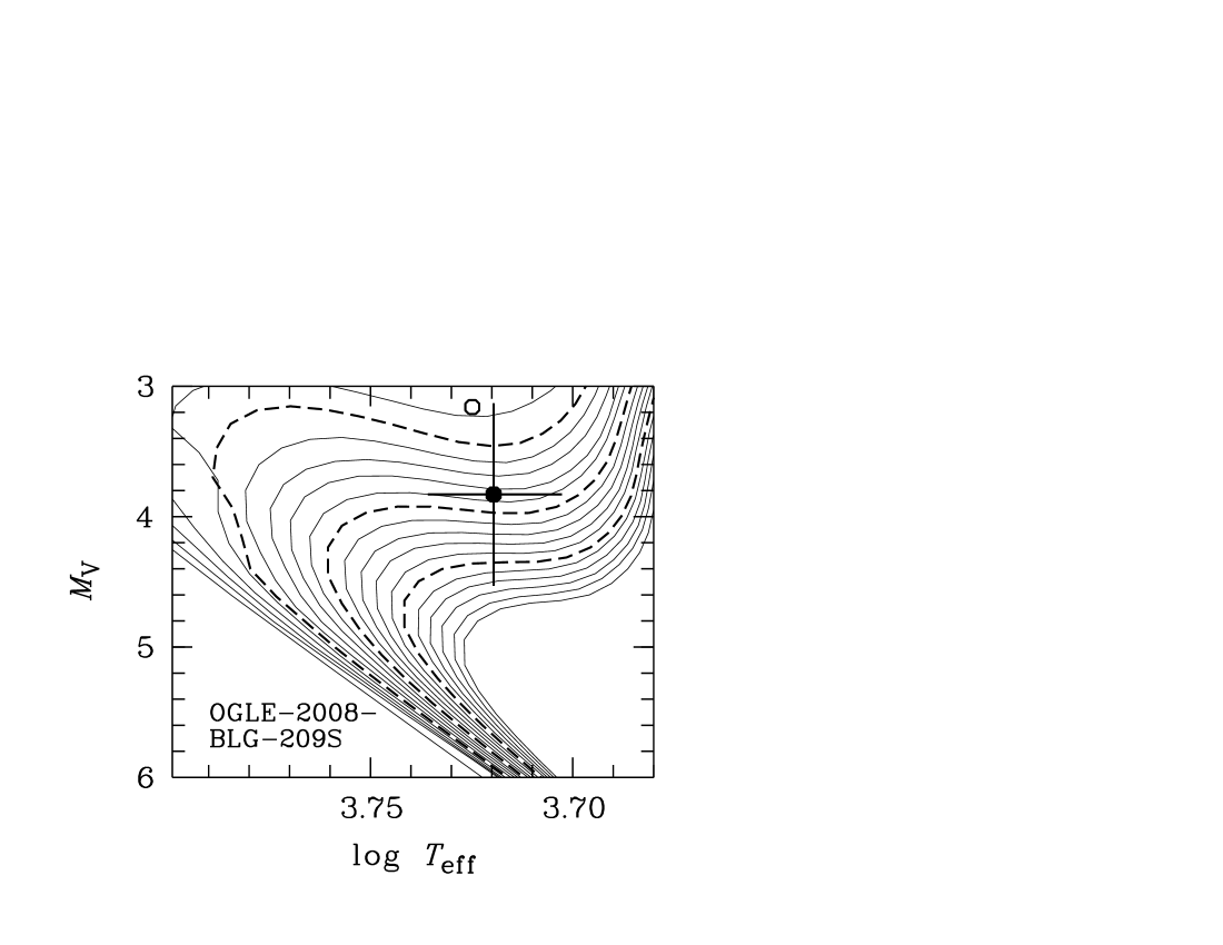
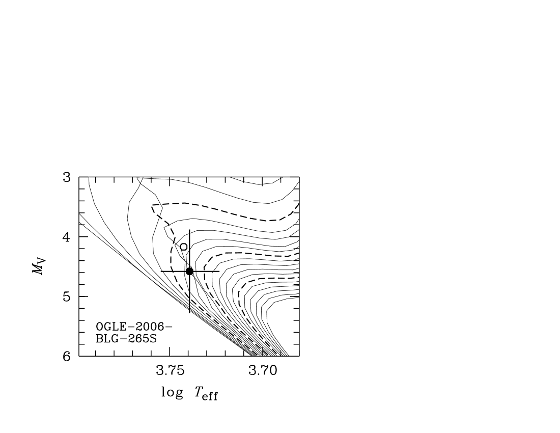
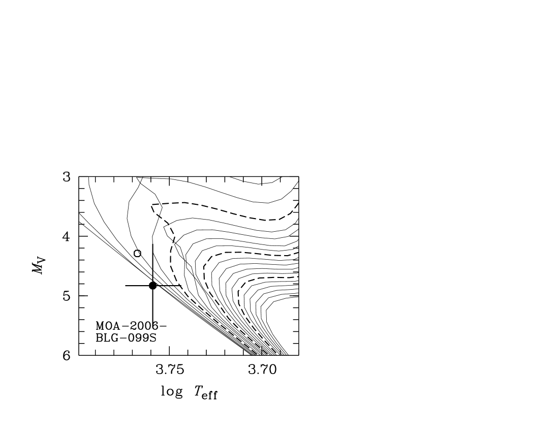
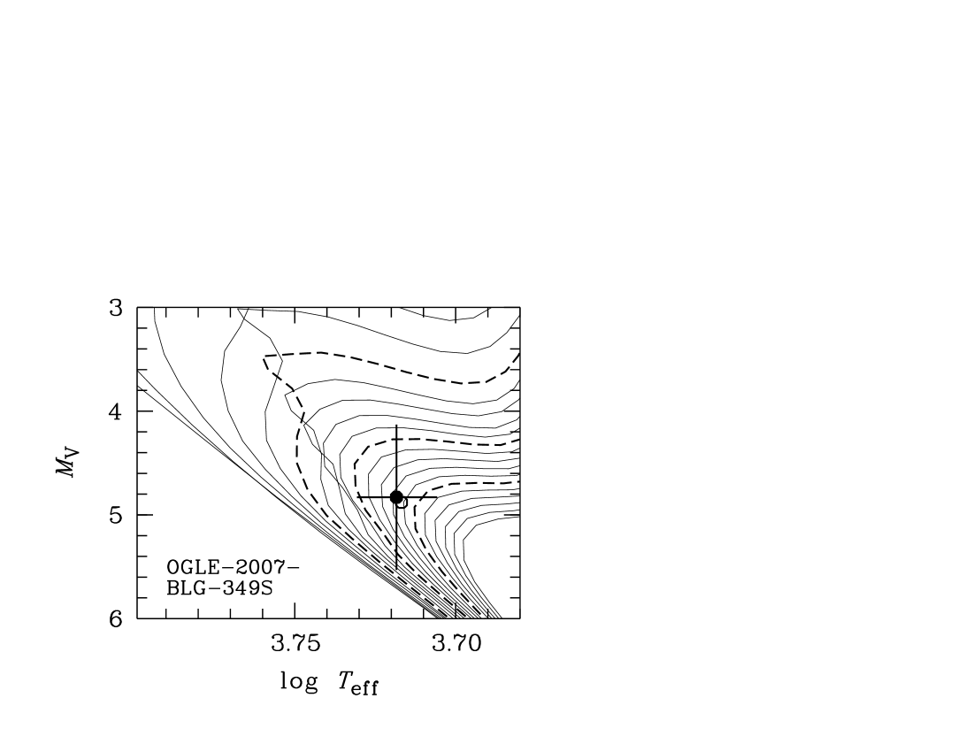
Figure 8: The Yonsei-Yale (Y²) isochrones (Yi et al. 2001; Kim et al. 2002; Demarque et al. 2004) that were used to estimate the stellar ages. Isochrones are plotted in 1 Gyr steps, with every 5 Gyr isochrone in dashed lines. For each target we used isochrones metallicities according to Table 3, and for OGLE-2008-BLG-209S also with an appropriate the $\alpha$-enhancement. Filled circles represent the stellar parameters derived from method 1 and open circles the stellar parameters from method 2. Error bars indicate uncertainties of 0.7 mag in $M_{\rm V}$ and 200 K in $T_{\rm eff}$.

When the final values of $\log g$, $T_{\rm eff}$, and $\xi_{\rm t}$ have been found we use the fundamental astrophysical relation $g\propto\mathcal{M}\cdot T_{\rm eff}^{4}/L$ to estimate the luminosity (and hence the apparent magnitude), assuming a distance of 8 kpc to the star. For methods 1 and 2 stellar ages were then estimated using the Yonsei-Yale isochrones (Yi et al. 2001; Kim et al. 2002; Demarque et al. 2004). Individual sets of isochrones with appropriate metallicities and $\alpha$-enhancements (in the case of OGLE-2008-BLG-209S) were calculated for the different stars. Ages were then read off from the best fitting isochrone in the $\log T_{\rm eff}$-$M_{\rm V}$ plane (see Fig. 8). Upper and lower limits to the ages were estimated from the error bars based on the uncertainties in $T_{\rm eff}$ and $M_{\rm V}$. For $T_{\rm eff}$ we adopt error bars of 200 K for OGLE-2008-BLG-209S, OGLE-2006-BLG-265S, and MOA-2006-BLG-099S, and 150 K for OGLE-2007-BLG-349S (see Sect. 5). The errors in $M_{\rm V}$ are difficult to estimate. Given the range of values by the different methods in Table 3 we adopt a value of 0.7 mag for the error in $M_{\rm V}$ for all four stars. This value is consistent with an uncertainty of 2 kpc in the adopted distance (see Sect. 6). These error bars are shown in the isochrone plots (see Fig. 8).

Also, stellar masses ($\mathcal{M}$) were determined from the evolutionary tracks by Yi et al. (2003) and are given in Table 3.

8 Stellar populations

Even if there are some discrepancies in the stellar parameters from the different methods that we have presented, they do produce results that are very similar in terms of abundance ratios. This is an encouraging result as it is the abundance ratios that are the main results used in discussions of the enrichment of heavy elements in a stellar population.

However, in order to put the new results for these four Bulge stars into context we will adopt the results from method 1. Method 1 is the method that most closely resembles the method used in Bensby et al. (2003, 2005) and Bensby et al. (2009, in prep), and will enable a differential comparison of the Bulge stars with a large sample of dwarf and subgiant stars in the nearby thin and thick discs. This choice is for consistency, and importantly, it does not make any judgement regarding which set of abundances is the most accurate.

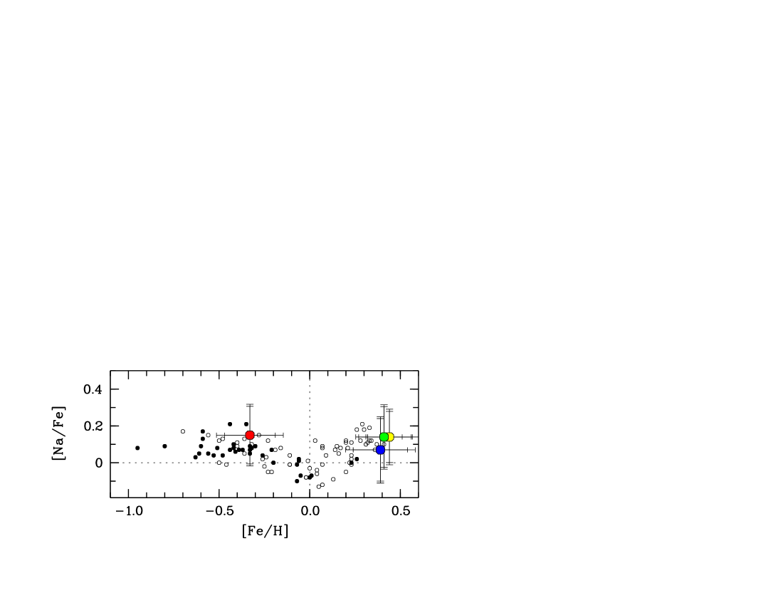
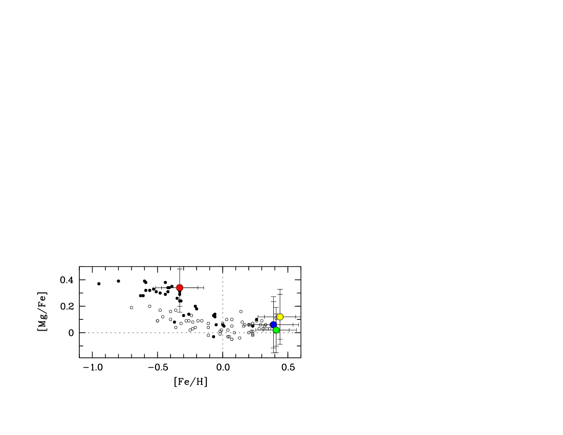
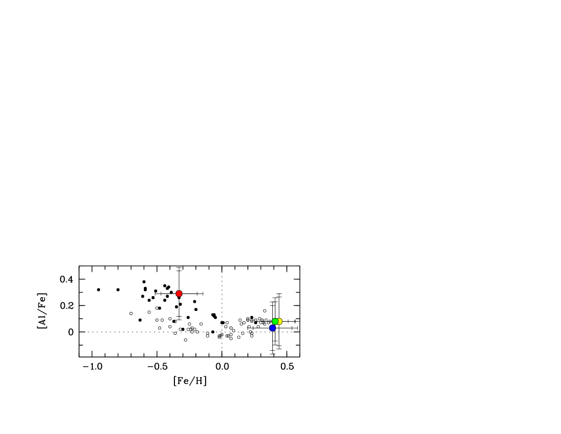
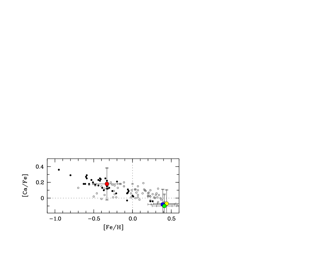
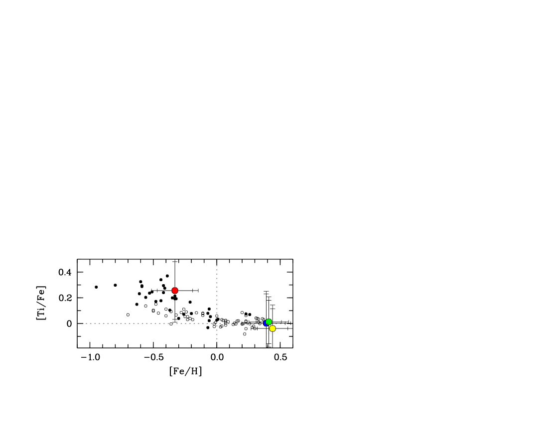
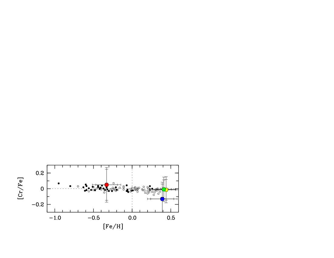
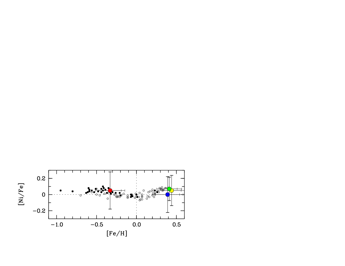
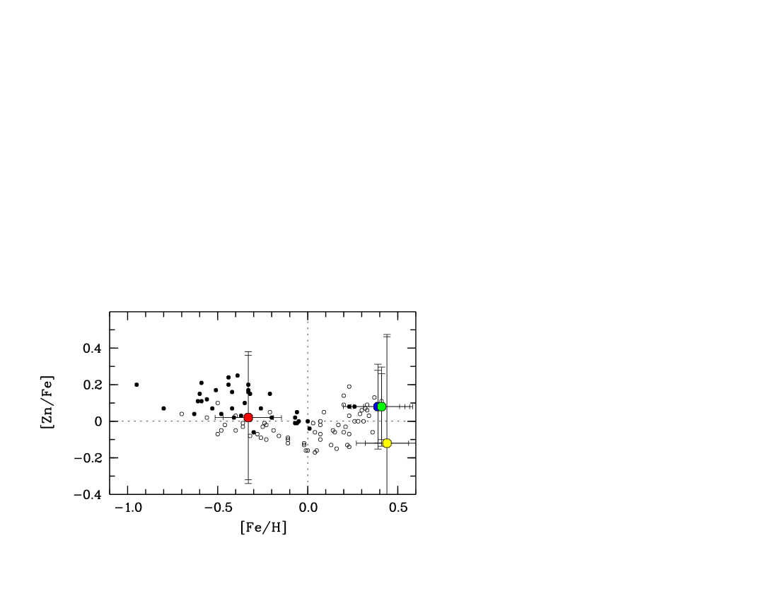
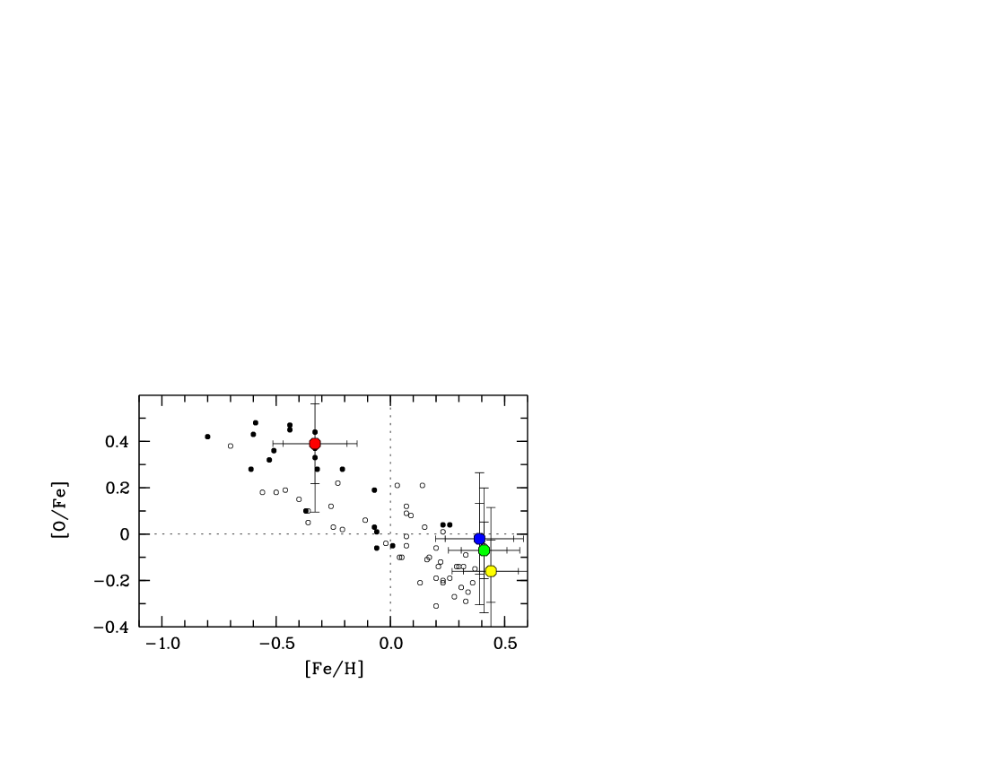
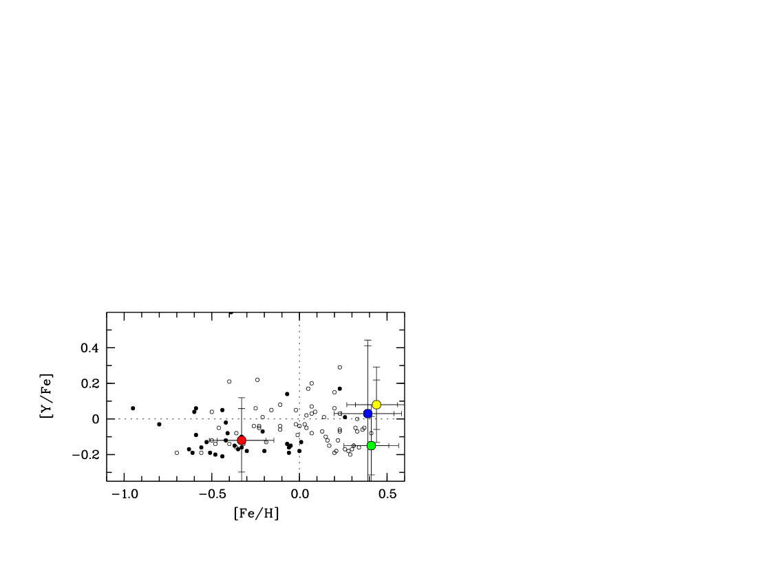
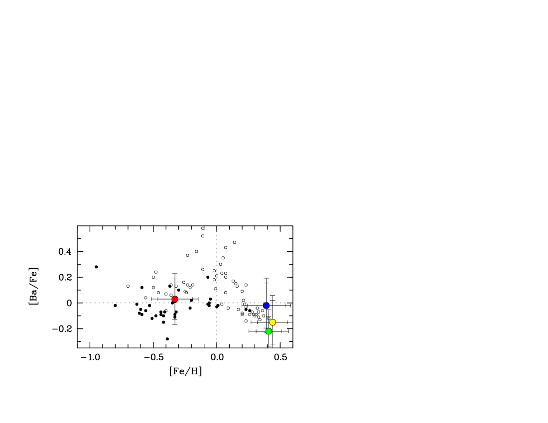
Figure 9: Abundance trends , [X/Fe] versus [Fe/H], for the thin and thick discs (taken from Bensby et al. 2003, 2005). Thin and thick disc stars are marked by open and filled circles, respectively. OGLE-2008-BLG-209S is marked by a red circle, OGLE-2006-BLG-265S by a yellow circle, MOA-2006-BLG-099S by a blue circle, and OGLE-2007-BLG-349S by a green circle. The error bars have two cross bars. The inner one represent the standard deviation of the mean abundance, and the outer cross bar represent the total error, i.e. standard deviation of the mean abundance and the uncertainty due to random errors in the stellar parameters, as given in Table 6, added in quadrature.

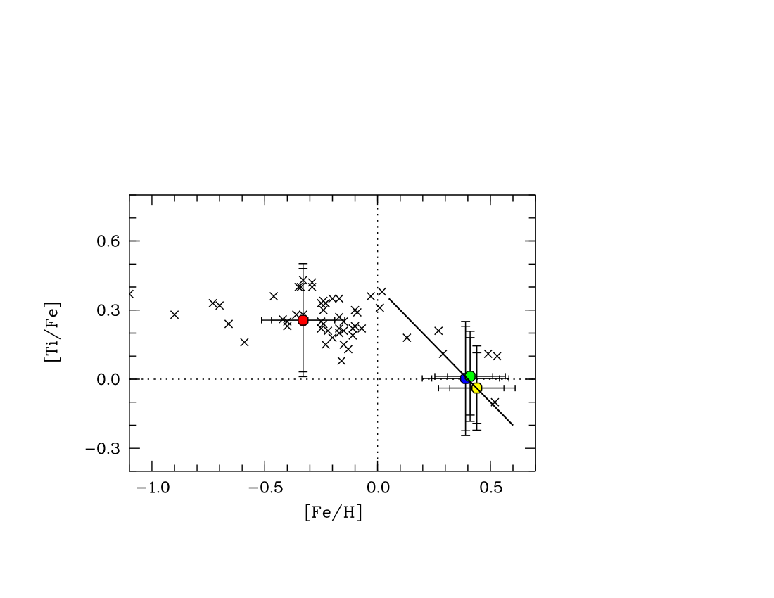
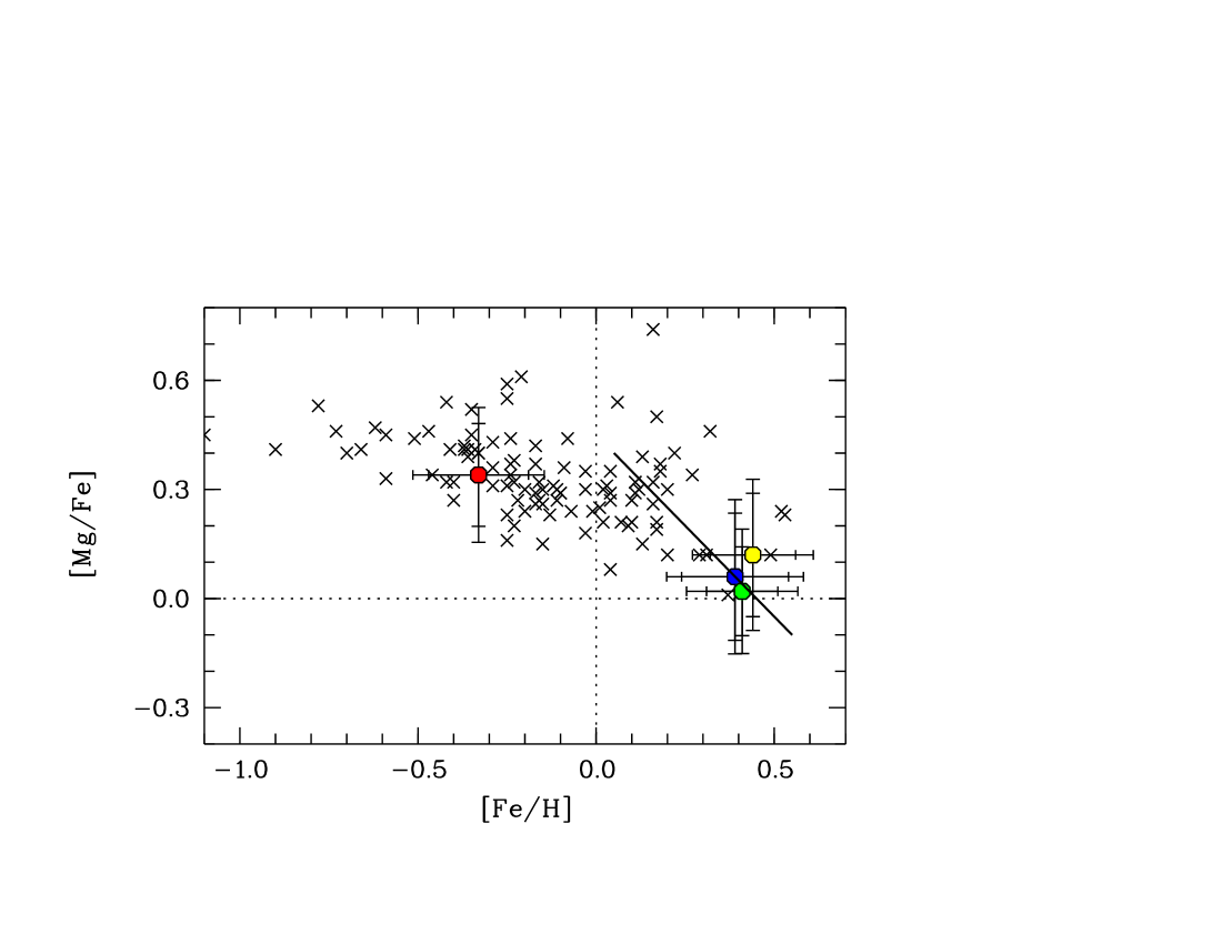
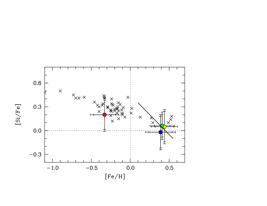
Figure 10: Elemental abundance trends in the Bulge based on giant stars (marked by crosses) (O, Mg, Si, and Ti from Rich & Origlia 2005; Rich et al. 2007; Fulbright et al. 2007; O and Mg from Lecureur et al. 2007; O from Meléndez et al. 2008). Nearby thick disc giant stars from Meléndez et al. (2008) are marked by filled circles. The four stars in this study are marked as in earlier figures. The diagonal line marks the maximum slope that the [$X$/Fe] ratio can decrease in order to reach the levels of the three metal-rich dwarf stars (the actual slope is however likely to be shallower, see discussion in Sect. 8.1.)

8.1 Elemental abundance trends in the Bulge

The Milky Way contains four major stellar populations; the halo, the thin and thick discs, and the bulge.

In Fig. 9 we show the thin and thick disc abundance trends from (Bensby et al. 2003, 2005). The stars of the thick disc have higher $\alpha$-to-iron abundance ratios than the stars of the thin disc. Specifically, the stars of the thick disc show a constant high $\rm[\alpha/Fe]$ ratio for low metallicities and all the way up to $\rm[Fe/H]\approx-0.4$ after which a down-turn in $\rm[\alpha/Fe]$ occurs, steadily declining towards solar values at solar metallicity. The stars of the thin disc, on the other hand, show a shallow decline in $\rm[\alpha/Fe]$ at lower metallicities that levels out at solar values at solar metallicities, where they merge with the thick disc trends.

In Fig. 9 we also show the results for the four dwarf/subgiant stars in the Bulge overplotted on the thin and thick disc abundance trends from Bensby et al. (2003, 2005). Generally, the abundance ratios for OGLE-2008-BLG-209S are similar to what is seen for the thick disc at the same [Fe/H]. Interestingly, the metallicity of OGLE-2008-BLG-209S ($-0.33$ dex) is where the separation between the thin and thick discs is the greatest. If anything, this demonstrates that the observed [$\alpha$/Fe] ratios in OGLE-2008-BLG-209S make it unlikely for it to be a thin disc star.

The three other Bulge dwarf stars, at super-solar metallicities, show abundance ratios for the $\alpha$-elements in close agreement with the metal-rich thin disc, i.e., close to the solar values ($\rm[\alpha/Fe]\approx 0$). Under the assumption that all four stars are all genuine members of the Bulge, this means that the abundance trends of the Bulge, somewhere in between these points, should show a significant decrease in the $\alpha$-to-iron ratios, signalling the onset of chemical enrichment from low-mass stars.

Figure 10 shows the abundance trends for O, Mg, Ti, and Si in the Bulge as traced by K and M giant stars (Rich & Origlia 2005; Rich et al. 2007; Lecureur et al. 2007; Fulbright et al. 2007; Meléndez et al. 2008), with the results for the microlensed dwarf and subgiant stars overplotted. The main chemical characteristics of the Bulge using giant stars can be summarised as follows: (1) The stellar formation history and chemical enrichment has been very fast. This is reflected by high [$\alpha$/Fe] ratios even at solar metallicities; (2) The [O/Fe] ratio starts to decline at roughly $\rm[Fe/H]\approx-0.3$, a signature of the onset of chemical enrichment by low-mass stars. (3) The [O/Fe]-[Fe/H] trends in the Bulge and the thick disc are similar (Meléndez et al. 2008). (4) Abundance trends based on other $\alpha$-elements such as Mg, Si, and Ti are similar to the oxygen trend, with the exception that the $\alpha$-enhancements for these elements, albeit slowly declining, tend to stay at somewhat higher levels with metallicity as compared to oxygen (see, e.g. Fulbright et al. 2007). Also, there are significantly fewer giant stars from these studies where abundances of Mg, and especially Ti and Si have been determined as compared to oxygen. (5) Generally the abundance ratios from the giant stars and the dwarf/subgiant stars seem to agree.

In order for a down-turn to occur in the first place in the [O/Fe]-[Fe/H] plot the oxygen enrichment (by massive stars) needs to decrease. The [O/Fe] ratio will then decrease, relative to Fe production, with [Fe/H] as a result of the continued Fe enrichment from low-mass stars. The maximum possible decrease of the [O/Fe] trend will occur if oxygen enrichment is shut off completely. The [O/Fe] ratio will then decrease by the same amount with which [Fe/H] increases. In the [O/Fe]-[Fe/H] plot this correspond to a line with a slope equal to $-1$. For simplicity, lets assume that this is the case. In Fig. 10 we show this line, and it is clear that, in order for the [O/Fe] ratio path to be able to decline to the observed [O/Fe] ratio in the three metal-rich Bulge dwarf stars, the oxygen production needs to be abruptly shut off at a metallicity not higher than $\rm[Fe/H]\approx-0.1$. It is of course unlikely that the oxygen enrichment should turn off “over-night”, instead it should be a gradual decrease, i.e. the slope of the line should be less than what we have indicated in Fig. 10. If so, it seems likely that the turn-over in the [O/Fe]-[Fe/H] trend as traced by dwarf and subgiant stars happens at approximately the same metallicity as for the giant stars, i.e. at $\rm[Fe/H]\approx-0.3$ to $-0.4$ (Meléndez et al. 2008). This also happens to be where we see the “knee” in the thick disc [$\alpha$/Fe]-[Fe/H] trends (Bensby et al. 2003, 2004, 2005). Similar lines have been drawn in the Mg, Si, and Ti plots in Fig. 10, indicating that the enrichment from low-mass stars started at $\rm[Fe/H]\approx 0$ (under the assumption that the enrichment of these elements from massive stars turned off abruptly).

8.2 A comparison of Bulge and inner disc dwarf stars

There is currently no in situ stellar sample that traces the inner disc regions of the Galaxy using detailed elemental abundances. A possible way to form a compatible sample would be to sample high-velocity stars with orbits that make them likely to have come from the inner parts of the Galactic disc. For instance, Pompéia et al. (2002) studied a sample of, so called, nearby “bulge-like” dwarf stars. These were defined as stars with highly eccentric orbits ($e>0.25$), that do not reach more than 1 kpc from the Galactic plane ($Z_{\rm max}<1$ kpc), and that have a maximum peri-galactic distance ($R_{\rm p}$) of 3 to 4 kpc. In Bensby et al. (2009, in prep) we have $\sim 700$ stars and 82 of those stars fulfil the “bulge-like” criteria by Pompéia et al. (2002). Figure 11 shows the [Ti/Fe]-[Fe/H] trends for these stars together with the four microlensed Bulge dwarf/subgiant stars. The observed trend for the “bulge-like” disc sample is very well defined with very little scatter. At sub-solar [Fe/H] there are no signs of [Ti/Fe] ratios seen in the local thin disc. This might not come as an surprise as we are picking stars on highly eccentric orbits, and if we were to trace the thin disc trend closer to the Galactic centre, those stars would likely be on on almost circular orbits and hence never cross the Solar orbit. It could also be that these disc stars on highly eccentric orbits belong to an inner disc population, distinct from the local thin and thick discs. This will be investigated further in Bensby et al. (2009, in prep.).

Plotting the microlensed Bulge dwarf and subgiant stars on top of the “bulge-like” disc sample (using the definition from Pompéia et al. 2002) in Fig. 11 we see that OGLE-2008-BLG-209S nicely fits into the trend and that the other three Bulge dwarf stars form a metal-rich extension of the trend.

8.3 The metallicity distribution of the Bulge

In Fig. 12 we plot the metallicity distribution of the 521 giant stars in the Bulge observed by Zoccali et al. (2008) in Baade’s window $(l,b)=(1.14,-4.18)$, and two other Bulge fields at $(l,b)=(0.21,-6.02)$ and $(l,b)=(0.0,-12.0)$. Also shown is the MDF of the 24 giant stars analysed by Fulbright et al. (2007), on which we have overplotted the metallicities of the four Bulge stars analysed in this work. Note that the distribution of the Fulbright et al. (2007) is not representative of the MDF in the Bulge. Their sample is designed to probe the full range of [Fe/H], not to be a representative sample. As can be seen the Bulge MDF based on the giant stars range from very low metallicities, $\rm[Fe/H]\approx-1.3$, to super-solar values comparable to the three previously published dwarf stars at $\rm[Fe/H]\approx 0.4$–0.5 (Johnson et al. 2007, 2008; Cohen et al. 2008). The average metallicity is $\rm[Fe/H]\approx-0.2$ (Zoccali et al. 2008).

An issues that has been discussed against results based on dwarf stars that have been microlensed is that the microlensing is affecting the spectrum of the source star and therefore we are not getting the right answer. This is why these stars (for some reason) are all very metal-rich (Zoccali et al. 2008). OGLE-2008-BLG-209S, the most recently analysed microlensed star, although being a subgiant, has a metallicity of $\rm[Fe/H]=-0.33$, and proves that it is indeed possible to find metal-poor microlensed stars. Also, since OGLE-2008-BLG-209S is approximately at the distance of the stars in Baade’s Window (because it’s very close spatially to BW, see Fig. 1), its metallicity is very compatible with the MDF of giant stars if they are spatially coincident (which is the case of OGLE-2008-BLG-209S and the giant stars by Zoccali et al. 2008). So this strengthens the idea that the analysis of microlensed dwarf and subgiant stars needs to be taken seriously.

8.4 Formation and chemical history of the Bulge

There are essentially three main formation scenarios for how galactic bulges may form.

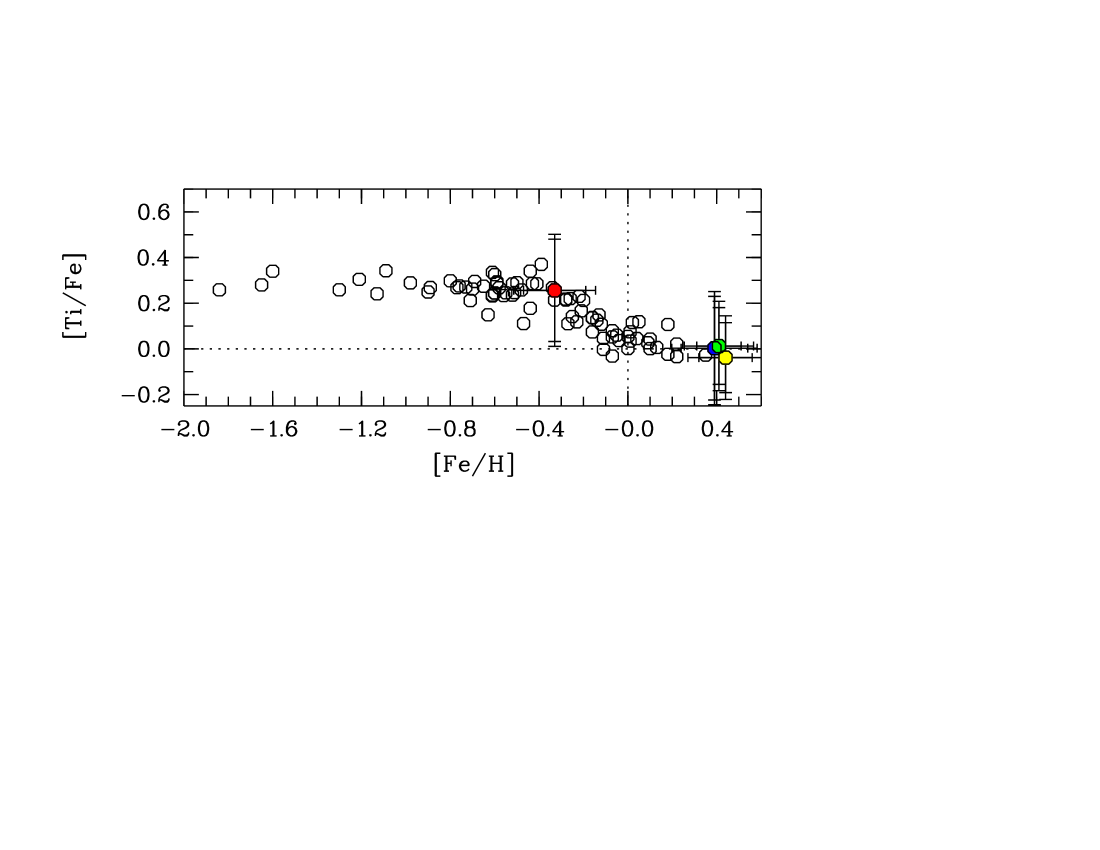
Figure 11: 82 nearby dwarf stars, selected from Bensby et al. (2009, in prep.), that have kinematic properties making them likely to come from the inner Galactic disc/Bulge. The kinematic criteria are the same as in Pompéia et al. (2002), i.e., $e>0.25$, $Z_{\rm max}<1.0$ kpc, and $R_{\rm min}<4$ kpc. OGLE-2008-BLG-209S (red circle), OGLE-2006-BLG-265S (yellow circle), and MOA-2006-BLG-099S (blue circle) have also been included.

Firstly, we have the classical scenario where the bulge form in the final phases of the monolithic collapse of the protogalactic cloud (Eggen et al. 1962). First the halo forms and as the collapse progresses also the bulge. The similarity between the distributions of angular momentum in the Bulge and halo suggest that this could be the case (Wyse & Gilmore 1992). Secondly, it is possible that bulges form from mergers in a $\Lambda$CDM Universe.

The outcome from these two scenarios is that the abundance trends in the Bulge could show many types of signatures. Depending on the star formation history, it is possible to get high $\alpha$-to-iron ratios extending to super-solar metallicities. However, as both of these scenarios happen in the very early phases of the formation history of the Galaxy, they would result in a Bulge that contain very old stars, as old as those found in the stellar halo. Even if not exclusively so, old stars are generally what is found in the Bulge (e.g. Feltzing & Gilmore 2000; Ortolani et al. 1995). However, in the collapse model, the average metallicity should increase as the collapse progresses inwards, resulting in metallicity gradients. Tentative evidence for a small metallicity gradient in the Bulge was found by Zoccali et al. (2008), see Fig. 12. For the hierarchical merger scenario in a $\Lambda$CDM Universe, where the in-falling “pieces” will be randomly distributed within the Bulge, no metallicity gradients are expected.

The third scenario is that bulges form through secular evolution, in which a bulge-like structure is built up through the slow rearrangement of energy and mass as a result of interactions between for instance a galactic bar and a galactic disc. If secular evolution dominates then it is quite likely that abundance trends in the bulge would mimic those of the central galactic disc as that is where the material and energy would come from to form the bulge. For the Milky Way bulge, the secular scenario has until recently been seen as quite unlikely because of the differing abundance patterns in the Bulge to those in the disc (e.g. Fulbright et al. 2007). However, recently Meléndez et al. (2008) carried out a truly differential study of Bulge and thin and thick disc giant stars and found that they are indeed very similar; the Bulge almost perfectly mimics the oxygen abundance trends of the nearby thick disc. Our results do not contradict this similarity.

As also pointed out by Meléndez et al. (2008), the similarity of the Bulge and the nearby thick disc oxygen trends, even though these two population clearly are spatially separated within the Galaxy, indicates that they have had very similar, but not necessarily the same, chemical enrichment histories. Observations of distant galaxies suggest that the secular scenario is very common (Genzel et al. 2008), and with the new abundance results we find that it is also a plausible scenario for the Milky Way bulge.

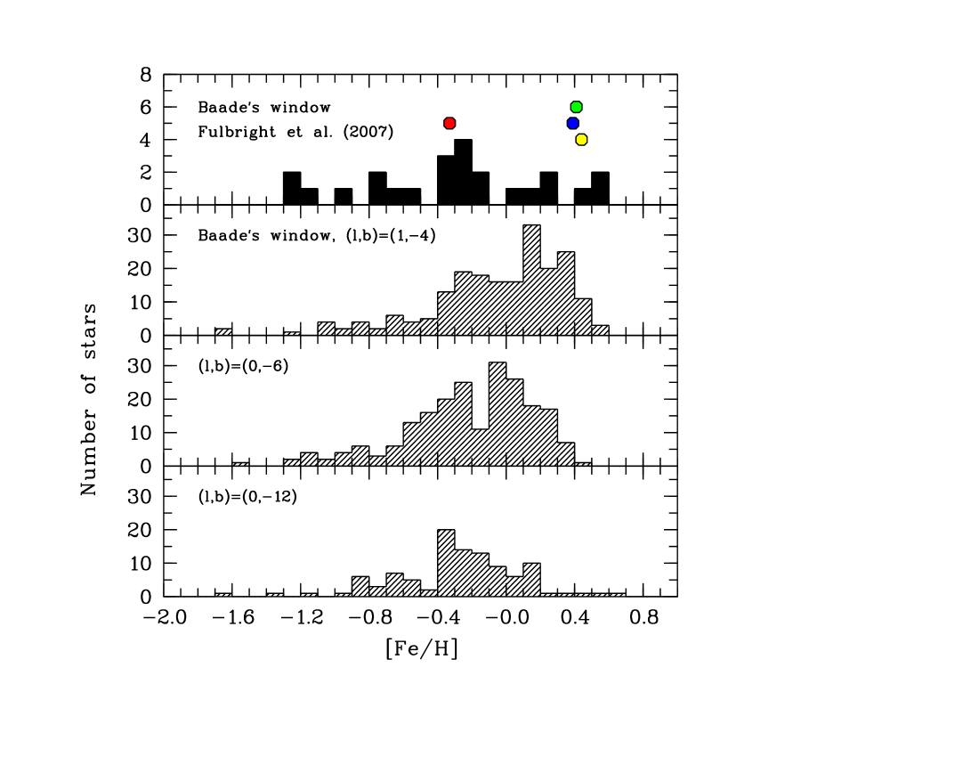
Figure 12: Metallicity distribution of the Bulge. Top panel shows metallicity histogram of the 24 giant stars from Fulbright et al. (2007), on which the metallicities of the four Bulge dwarf/subgiant stars analysed in this work, marked as in previous plots (arbitrarily shifted vertically). The three bottom panels show the MDF of the giant stars in three different Bulge fields from Zoccali et al. (2008). The $(l,b)=(1.14,-4.18)$ field has 244 stars, the $(l,b)=(0.21,-6.02)$ field 213 stars, and the $(l,b)=(0.0,-12.0)$ field 104 stars.

9 Summary

We have performed a detailed elemental abundance analysis of OGLE-2008-BLG-209S, a microlensed subgiant star in the Bulge. In contrast to the three previously published microlensed Bulge dwarf stars, that all turned out to be extremely metal-rich, having metallicities greater than $\rm[Fe/H]>0.35$ (Johnson et al. 2007, 2008; Cohen et al. 2008), OGLE-2008-BLG-209S has a more modest sub-solar metallicity of $\rm[Fe/H]\approx-0.33$. Interestingly, the metallicity of OGLE-2008-BLG-209S is where the separation in the [$\alpha$/Fe] ratio between the thin and thick disc stars is the greatest. Furthermore, the abundance pattern of OGLE-2008-BLG-209S is similar to what is found in nearby thick disc dwarf stars and what is found in giant stars in the Bulge, i.e. enhanced $\alpha$-to-iron ratios (e.g., O, Mg, Si, Ca, Ti).

We have also carried out a re-analysis of the three microlensed dwarf stars, previously published by Johnson et al. (2007, 2008) and Cohen et al. (2008). This was done in order to get a homogeneous sample of Bulge dwarf and subgiant stars analysed with the same methods as for the large sample of nearby thin and thick disc dwarf stars by Bensby et al. (2003, 2005). With some exceptions we see good agreement in abundances between our results for MOA-2006-BLG-099S, OGLE-2006-BLG-265S, OGLE-2007-BLG-349S and those in Johnson et al. (2007, 2008); Cohen et al. (2008). For instance, the metallicity of OGLE-2006-BLG-265S is lower in our new analysis ($\rm[Fe/H]=+0.44$) than what Johnson et al. (2007) found ($\rm[Fe/H]=+0.56$).

The three stars for which we could estimate ages are (using method 1) 8.5 Gyr, 7.5 Gyr, and 13 Gyr old, respectively. These ages are higher than what we see for thin disc stars at these metallicities. However, the stars of the thick disc are found to be older than the stars of the thin disc. This could suggest that the metal-rich stars of the Bulge have ages comparable to what we see in the metal-rich thick disc (at solar metallicities, Bensby et al. 2007). It should be cautioned that individual ages based on isochrones could be subject to substantial systematic and random uncertainties. Therefore, ages for many more bulge dwarf and subgiant stars must be determined before firm conclusions can be drawn.

We have also considered several methods in analysing the stars and find that elemental abundance ratios based on the methods are in good agreement, showing small or negligible differences. We would like to stress that the differences between the methods we used to get abundances from Bulge dwarf stars have been quantified, and that our investigation shows that one always should be very careful in combining information from differnet studies unless all ”facts” are clearly explained (such as the solar abundances used for normalisation, etc.).

The above results are based on less than a handful of dwarf/subgiant stars. It is very important to further confirm these results with more observations. However, high-magnification microlensing events, that currently seem to be the only feasible way of getting good quality high-resolution data of Bulge dwarf stars, are very rare. Out of the yearly thousands of detected microlensing events from the OGLE monitoring of the Bulge, only a dozen are dwarf events. As it is impossible to know beforehand when these will occur, it is necessary to have a flexible observing schedule to be able to catch them. As such, the Rapid Response Mode with the UVES spectrograph on the Very Large Telescope should be optimal.