Mapping the Galactic Halo VIII: Quantifying substructure

Abstract

We have measured the amount of kinematic substructure in the Galactic halo using the final data set from the Spaghetti project, a pencil-beam high-latitude sky survey. Our sample contains 101 photometrically selected and spectroscopically confirmed giants with accurate distance, radial velocity, and metallicity information. We have developed a new clustering estimator: the “4distance” measure, which when applied to our data set leads to the identification of one group and seven pairs of clumped stars. The group, with six members, can confidently be matched to tidal debris of the Sagittarius dwarf galaxy. Two pairs match the properties of known Virgo structures. Using models of the disruption of Sagittarius in Galactic potentials with different degrees of dark halo flattening, we show that this favors a spherical or prolate halo shape, as demonstrated by Newberg et al. using the Sloan Digital Sky Survey data. One additional pair can be linked to older Sagittarius debris. We find that 20% of the stars in the Spaghetti data set are in substructures. From comparison with random data sets we derive a very conservative lower limit of 10% to the amount of substructure in the halo. However, comparison to numerical simulations shows that our results are also consistent with a halo entirely built up from disrupted satellites, provided that the dominating features are relatively broad due to early merging or relatively heavy progenitor satellites.

1. Introduction and Outline

In modern, cold dark matter dominated, cosmological models structure builds up hierarchically, i.e., small structures collapse first and then merge together to form larger structures. If such processes also take place on galactic scales, we would expect to see merger debris in the stellar halos of galaxies (e.g., Bullock & Johnston 2005). We should find substructures there that remain coherent in phase space for many gigayears (Johnston et al. 1996, Helmi & White 1999). This prediction has led to intensive searches, especially in the Milky Way, and to the development and exploitation of several surveys. These include, for example, large photometric surveys like the Sloan Digital Sky Survey (SDSS Adelman-McCarthy et al. 2007) and Two Micron All Sky Survey (2MASS Skrutskie et al. 2006), but also smaller surveys that use more distinct halo tracers like RR Lyrae variables (e.g., QUEST, Vivas et al. (2004); SEKBO, Moody et al. (2003)), or halo red giant stars such as the Spaghetti survey, first described in Morrison et al. (2000).

These surveys have produced the much sought after observational evidence for late merging in the outer halo of our Galaxy, which is presumably associated with its hierarchical formation. The Magellanic Stream (Mathewson et al. 1974) and especially the Sagittarius dwarf galaxy (Ibata et al. 1994, Majewski et al. 2003) that is being tidally stripped by our Milky Way, are two smoking gun examples. Other large-scale features found in the Galaxy are the Monoceros stream, a relatively broad stream of stars of debated origin (Newberg et al. 2002, Ibata et al. 2003, Martin et al. 2004, Peñarrubia et al. 2005) and several substructures in the direction of Virgo (Vivas et al. 2001, Newberg et al. 2002, Zinn et al. 2004, Jurić et al. 2008, Duffau et al. 2006, Newberg et al. 2007, Keller et al. 2008). Various small substructures have been found as well (e.g., Clewley & Kinman 2006, Belokurov et al. 2007a), of which a remarkable example is the relatively narrow “Orphan Stream” (Belokurov et al. 2007b, Grillmair & Dionatos 2006). The existence of substructure is not restricted to the Milky Way, but is also found in the stellar halos of other galaxies (e.g., Shang et al. 1998, de Jong et al. 2007; 2008, Martínez-Delgado et al. 2008; 2009), most notably in M31 where a prominent stellar stream and a wealth of smaller tidal features have been detected (Ibata et al. 2001a; 2007).

Although many substructures have been uncovered (e.g., Belokurov et al. 2006), their role in the formation of the Milky Way galaxy is still unclear. Is late accretion a dominant or a minor factor in the buildup of the halo? Is the halo dominated by a smooth component which underlies the substructures we find? Or do the discovered substructures represent the tip of the iceberg and is the whole galaxy halo in fact the result of merged (stellar) structures?

Most surveys carried out so far have been analyzed in a rather qualitative manner, and so do not give a direct answer to these very fundamental questions. The first thorough attempt at quantifying this process was carried out by Bell et al. (2008). They analyzed the amount of substructure in the spatial distribution of the stellar halo using $\sim$4 million color-selected main-sequence turnoff stars in the SDSS. The magnitude limits of this survey correspond to distances of $\sim$35 kpc from the Sun. They found that fractional rms deviations on scales $\geq$ 100 pc from the best-fitting smooth halo model are $\geq$ 40%. Hence they concluded that the stellar halo is highly structured, which is consistent with a scenario in which merging is an important factor in the buildup of the halo.

In this paper, we statistically quantify the amount of substructure in the halo, but now we combine spatial and kinematical data from the Spaghetti survey. As we will show below, the addition of kinematical data greatly improves our ability to identify substructure. Additionally, our survey traces the halo using giant stars to much larger distances of $\sim$100 kpc. To achieve our goal, we have developed a new substructure estimator. This 4distance estimator works in a four-dimensional space defined by the spatial coordinates and radial velocities of stars. As we shall show below, it particularly is suitable for finding substructures with similar sky position, distance and radial velocities.

Our paper is organized as follows. In Section 2 we briefly discuss the properties of the final Spaghetti data set (we defer a more detailed description to H.L. Morrison et al., in preparation). In Section 3 we present our substructure estimator and apply it to this data set. Our results are compared with simulations of stellar halos built up completely from accreted satellites in Section 4. In Section 5 we discuss whether any of the substructures found in our analysis can be related to known structures. We discuss and summarize our results in Section 6 and 7.

2. The data set

The Spaghetti survey is a pencil-beam survey of high-latitude fields that was completed in 2006. Washington photometry was used to preselect red giant candidates (see for more details Morrison et al. 2000, Dohm-Palmer et al. 2000, Morrison et al. 2001). These candidates were then followed-up spectroscopically as described in detail in Morrison et al. (2003). By measuring the strength of the Ca II K, Ca I $\lambda 4227$ and Mg $b/$H features, metal-poor dwarfs and halo giants can be distinguished in order to obtain a clean sample of K giants in the halo.

All spectroscopically confirmed giant stars are included in the Spaghetti data set. This final data set consists of 101 giants, from 13 separate spectroscopic runs. Two giants have distances $\geq$ 100 kpc, 33 of them have distances over 30 kpc. The typical errors on distance are 15%, on radial velocity 10–15 km s^-1 and on metallicity 0.25–0.3 dex. The sky coverage, distances, radial velocities, metallicities and corresponding errors of the data set will be presented in a forthcoming paper (Morrison et al., in preparation).

3. The 4distance

We expect debris from a merged satellite to remain spatially coherent in the outer halo (see, for example, the numerical simulations of satellite accretion by Johnston et al. 1996). Even when spatial structure is no longer apparent, the debris from the merged satellite can still be recognized in velocity space (Helmi & White 1999). Therefore, stars from the same parent object should be clustered in phase space.

For the 101 giants in our data set we possess information on four of the six phase space components: the spatial components (galactic longitude, galactic latitude and distance), and radial velocity. With these four components, we can define a measure of clustering by computing a distance in a four-dimensional space for every pair of stars in our data. We use
$l$ = galactic longitude,
$b$ = galactic latitude,
$d$ = distance to the Sun,
$v$ = $v_{GSR}$ = line-of-sight velocity corrected for solar and local standard of rest (LSR) motions,
$\phi$ = angular distance on the sky between the two stars.

We now define our 4distance between two stars $i$ and $j$ as follows:

$$4dist_{ij}=(w_{\phi}\phi^{2}_{ij}+w_{d}(d_{i}-d_{j})^{2}\\ +w_{v}(v_{i}-v_{j})^{2})^{0.5},$$

where

$$\cos\phi_{ij}=\cos b_{i}\cos b_{j}\cos(l_{i}-l_{j})+\sin b_{i}\sin b_{j}.$$

Stars with small separations in this metric are expected to come from the same object.

While the galactic longitude and latitude are incorporated as part of the angular separation, the other components are used completely independently in the final 4distance measure. The quantities $w_{\phi}$, $w_{d}$, and $w_{v}$ are used to weigh the various components, first normalizing by the range of this quantity (the largest possible angular separation is $\pi$, distance 130 kpc and velocity 500 km s^-1) and then by our observational errors on distance ($d_{err}$) and line-of-sight velocity ($v_{err}$). In the distance component, the relative error $d_{err}/d$ is used since distance errors scale with the distance itself:

$$w_{\phi}=\Bigl{(}\frac{1}{\pi}\Bigr{)}^{2},\ \ w_{d}=\Bigl{(}\frac{1}{130}\Bigr{)}^{2}\displaystyle\frac{\displaystyle\Bigl{(}\frac{d_{err}(i)}{d(i)}\Bigr{)}^{2}+\displaystyle\Bigl{(}\frac{d_{err}(j)}{d(j)}\Bigr{)}^{2}}{2\Bigl{\langle}{\displaystyle\frac{d_{err}}{d}}\Bigr{\rangle}^{2}}$$ (1)

$$w_{v}=\Bigl{(}\frac{1}{500}\Bigr{)}^{2}\,\displaystyle\frac{v^{2}_{err}(i)+v^{2}_{err}(j)}{2\langle{v_{err}}\rangle^{2}}.$$ (2)

We find that the group-finding algorithm is quite insensitive to small changes in the weighting factors. Multiple possibilities have been explored, using several combinations of normalizing factors as well as dependence of errors, which did not affect the key results presented in this paper by more than a few percent.

3.1. Choosing a relevant binsize

We expect stars with small 4distance to be possible stream members. However, the actual values of 4distance for stream members will depend on a number of factors including the spatial sampling of the Spaghetti survey.

We construct random samples in order to assess how often small values of 4distance will occur by chance. To mimic our data set as much as possible, we create random sets in which each star in the original sample preserves its galactic longitude and latitude, but is randomly supplied with a different (reshuffled) velocity and independently with a different observed distance. In this way, we break any correlations in the data while maintaining its global properties. We call two stars that are within a certain 4distance a pair. By comparing the total number of pairs at a certain 4distance in both the data and 1000 randomized data sets, the significance in the number of pairs with small 4distance can be investigated. This comparison is shown in Figure 1; the error bars in the bottom panel are Poissonian.

Figure 1.— Top panel shows the cumulative number of pairs found as a function of $4dist$ for the Spaghetti data (black) and for the average of 1000 random sets (gray). The bottom panel shows the cumulative correlation function defined as the number of pairs in the data divided by the average number of random pairs below a certain $4dist$.

The number of pairs within a certain 4distance measures the clumpiness of the data at that particular scale. For all scales up to a $4dist$ of 0.13 plotted in Figure 1, the amount of clumpiness in the data is larger than in the randomized set. Based on Figure 1, we decide to investigate in more detail data pairs at two different scales. First, we would like to choose a $4dist$ within which the ratio of data pairs to random pairs is sufficiently large that our data pairs have a high chance of being real. Second, we want to avoid throwing away pairs by being too restrictive.

We first focus on a $4dist$-scale of $0.05$. Table 1 lists what this scale corresponds to in physical units. For a pair of stars with exactly the same radial velocity and distance from the Sun, a $4dist=0.05$ implies a maximum separation on the sky of $9^{\circ}$. At a distance of 5 kpc this corresponds to a physical size of 0.8 kpc, while at 50 kpc it would be 10 times larger. Note however that the values given in the Table are clearly upper limits, since no two stars will have the exact same values of the remaining coordinates.

For a $4dist\leq 0.05$, 12 pairs are found in the data set and on average just $\sim 5$ pairs in the random sets. The bottom panel in Figure 1 shows that for $4dist\geq 0.05$ the significance decreases. Supplementary to the core structures defined by the pairs found at $4dist\leq 0.05$, we also explore if other stars in our data set have $4dist\leq 0.08$ such that they could be added to these core structures.

Table 1Maximum separations in the metric for $4dist=0.05$

Maximum separation in	for $4dist=0.05$
Angle on the sky	$9^{\circ}$
Distance	6.5 kpc
Radial velocity	25 km s-1

3.2. Pairs and groups

Some of the 12 pairs with $4dist\leq 0.05$ can be combined to form larger groups. We define a group of stars when every member has a $4dist\leq 0.05$ with at least one other member of the group. This we call the friends-of-friends criterion. For each star_i and star_j they belong to the same group if for:

$$\textrm{star}_{i}\ \exists\ \textrm{star}_{j}\ /\ 4dist_{ij}\leq\epsilon,\ \textrm{where}\ \epsilon=0.05$$ (3)

Using this criterion one large group of five members is found. This leaves seven pairs that cannot be extended to groups with more members. We subsequently look at the added substructure within a $4dist$ of 0.08. All stars in the original core group of five are within a $4dist$ of 0.08 with every other member of the group, which strengthens the significance of this group. An extra member was found within a $4dist$ of $0.08$ of two of these stars. Therefore, this leaves us with one group of six stars and seven independent pairs. The properties of the final group and pairs are given in Table 2 and are shown in Figures 2 (on the sky), 3 (velocity vs. distance) and 4 (metallicity vs. distance).

Table 2Positional, velocity and metallicity information for all giants in groups and pairs.

	RA(2000)	DEC(2000)	$l$	$b$	[Fe/H]	D⊙	Vr⊙	VGSR	Verror
	h:m:s	∘:’:”	(deg)	(deg)	(dex)	(kpc)	(km s-1)	(km s-1)	(km s-1)
1	15:15:27.06	+3:56:02.3	5.3037	48.5534	–1.41 $\pm$ 0.29	52.36 $\pm$ 7.34	23.7	49.5	8.6
1	14:53:30.96	+1:25:42.2	356.8098	51.0609	–1.87 $\pm$ 0.30	50.66 $\pm$ 8.53	18.6	22.6	15.0
1	14:52:42.98	+1:23:24.2	356.5443	51.1777	–1.29 $\pm$ 0.26	51.30 $\pm$ 4.46	29.6	33.0	9.2
1	14:52:50.78	+1:29:46.6	356.7020	51.2284	–2.33 $\pm$ 0.31	58.70 $\pm$ 3.87	9.2	13.0	4.7
1	14:52:40.14	+1:03:18.8	356.1503	50.9520	–1.65 $\pm$ 0.26	51.95 $\pm$ 5.77	49.2	51.6	11.7
1	14:31:46.61	+10:46:49.5	3.0593	61.2957	–1.54 $\pm$ 0.35	48.23 $\pm$ 6.58	26.4	43.3	22.5
2	15:44:49.80	–0:22:12.8	6.7604	40.1085	–0.91 $\pm$ 0.39	8.87 $\pm$ 1.47	–34.3	–1.8	4.8
2	15:44:53.56	+0:05:52.4	7.2636	40.3766	–0.98 $\pm$ 0.39	7.44 $\pm$ 1.12	–8.8	25.1	3.2
3	15:44:45.29	–0:17:03.4	6.8354	40.1752	–1.11 $\pm$ 0.25	8.12 $\pm$ 0.82	48.9	81.6	5.9
3	15:42:47.40	–0:07:00.2	6.6228	40.6683	–2.41 $\pm$ 0.25	7.51 $\pm$ 0.86	72.7	104.6	6.3
4	15:39:05.02	+10:28:36.5	18.2709	47.2382	–0.90 $\pm$ 0.26	6.30 $\pm$ 0.78	–21.1	38.6	3.4
4	15:40:23.26	+10:13:46.6	18.1812	46.8380	–0.93 $\pm$ 0.39	3.94 $\pm$ 0.46	–16.9	42.9	3.2
5	3:26:11.85	–2:29:40.1	186.0313	-45.5498	–2.71 $\pm$ 0.25	23.62 $\pm$ 1.78	–18.1	–46.8	17.7
5	3:25:31.69	–1:45:08.8	185.0501	-45.2278	–1.31 $\pm$ 0.23	25.11 $\pm$ 2.56	–29.3	–55.4	5.3
6	10:34:00.09	–19:00:13.8	263.3616	33.1049	–1.28 $\pm$ 0.26	27.42 $\pm$ 2.66	378.3	193.9	8.0
6	10:54:02.91	–19:01:19.0	268.0987	35.7882	–1.08 $\pm$ 0.28	30.18 $\pm$ 3.83	382.2	203.6	17.0
7	12:32:11.52	–1:03:44.5	292.8318	61.4314	–1.29 $\pm$ 0.25	13.00 $\pm$ 1.22	–45.3	–136.4	5.0
7	12:56:08.49	–2:16:23.8	305.3242	60.5766	–1.43 $\pm$ 0.32	16.13 $\pm$ 1.82	–39.9	–121.1	13.0
8	12:54:54.56	–2:20:29.4	304.6941	60.5184	–1.34 $\pm$ 0.26	17.00 $\pm$ 1.73	255.7	173.6	5.4
8	12:56:14.74	–1:30:17.8	305.4380	61.3434	–1.46 $\pm$ 0.56	13.16 $\pm$ 2.73	229.8	150.9	6.0

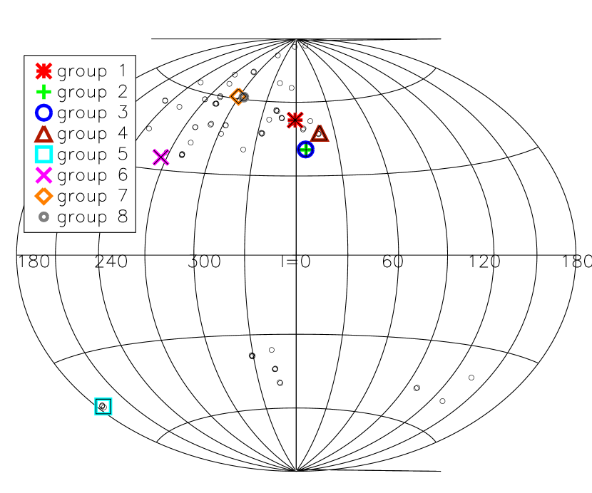
Figure 2.— Sky distribution of the data set highlighting the location of the group and pairs found. Note that pairs 2 and 3 are overlapping on the sky, but they possess very different velocities.

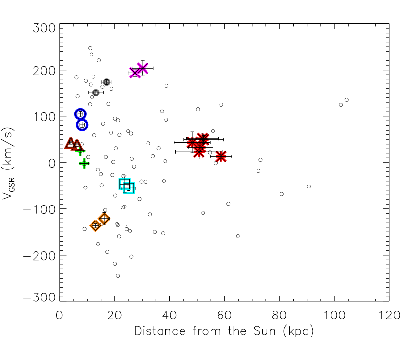
Figure 3.— Distribution of the data set in galactocentric velocity (defined as line-of-sight velocity corrected for the solar motion and LSR) vs. distance with the group and pairs overplotted. The color coding (in the online version) and the symbols are the same as in Figure 2.

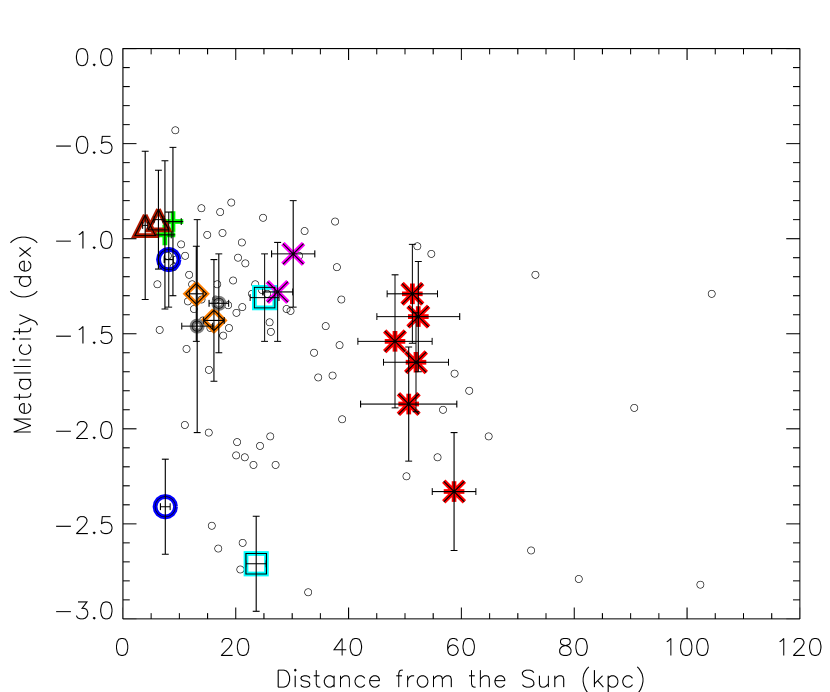
Figure 4.— Distribution of the data set in metallicity vs. distance with the group and pairs overplotted in different colors. The color coding (in the online version) and the symbols are the same as in Figure 2.

3.3. Significance of the group and pairs

We now investigate the significance of the group and pairs. At both levels, $4dist\leq 0.05$ and $4dist\leq 0.08$, more substructure is found in the data set compared with the random sets. The core group of five members, found at the $4dist\leq 0.05$ level, stands out very significantly. We find a probability of about 1% to obtain such a large group in our random sets. The probability of finding pairs in our random sets is significantly higher, in almost all random sets at least one pair is found, but only in $\sim$1% of our random sets we find the same high fraction of stars to be paired. This implies that, while finding some pairs in a random set has a high probability, finding 19 stars in pairs at a level of $4dist\leq 0.05$, as we do in our data set, is a highly improbable event.

The metallicity of the stars is not used as a criterion to select pairs. While a certain spread in metallicity can be expected in stars originating from a disrupted satellite, the observed spread gives additional information about the probability that a group or pair is real. In our case especially pair 3 and pair 5 show a large range in metallicity, as can be seen in Figure 4. For the other pairs however, the fact that their members are close in metallicity as well as in sky position and radial velocity makes them, and our selecting algorithm, more credible.

4. Simulated data sets

We would like to constrain what fraction of the stellar halo has been built from accreted satellites using the results from the previous section. To this end, and to test the 4distance method used, we compare our data set to a simulation of a halo which is entirely the result of disrupted dwarf galaxies. For this purpose we use the simulations from Harding et al. (2001) that model the destruction by the Milky Way galaxy of a $10^{7}M_{\odot}$ satellite on different orbits.

Forty of the original satellite simulations were re-sampled so that each particle corresponds to one halo K giant. This leaves nearly 8700 particles per satellite. The distribution of these K-giant simulations after 10 Gyr is shown in Figure 5.

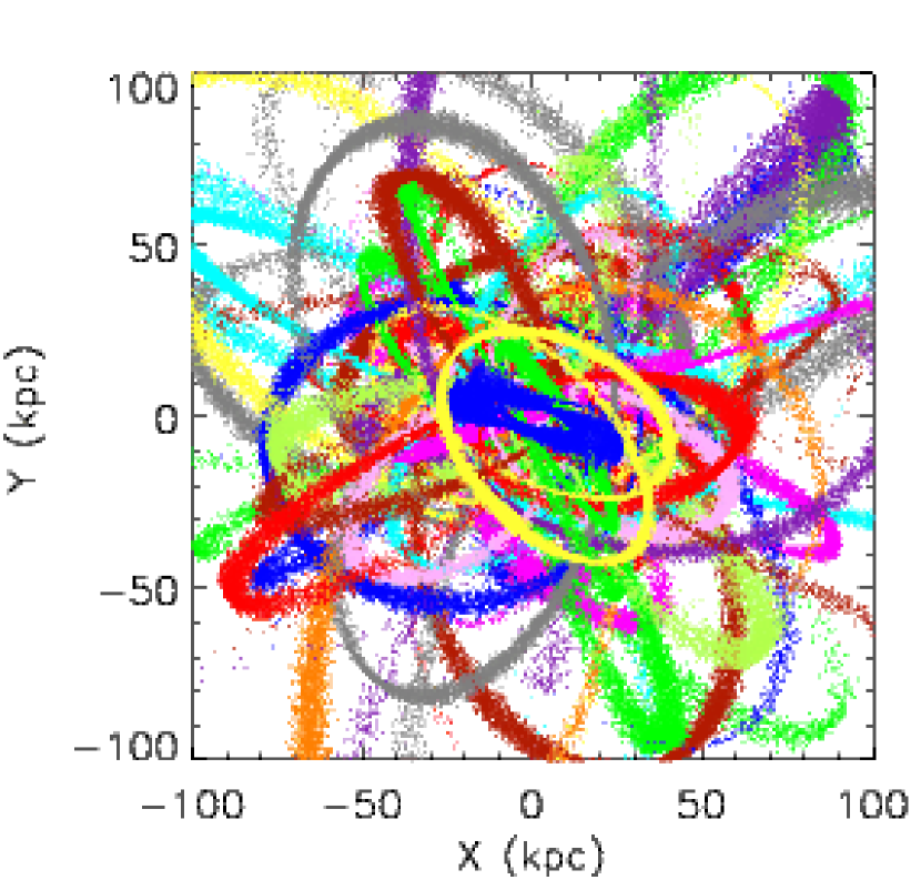
Figure 5.— X – Y projection showing the distribution of streams in our simulated stellar halo built up from 40 disrupted satellites.

To create a halo built up completely out of disrupted galaxies, the endpoints of the simulations (i.e., evolved for 10 Gyr) are used. From this sample of over 340,000 simulated ‘giants’ we draw subsets of 101 stars by requiring that the observed sky distribution, distance and radial velocity distribution of the Spaghetti data set are matched within certain binsizes. In this manner, 30 simulated data sets are drawn which closely resemble the Spaghetti observations.

4.1. Substructure in the simulated data sets

We look for substructure in the simulated data sets using the 4distance method. In order to make a fair comparison, the simulated ‘giants’ are convolved with errors, to mimic the observational uncertainties. For the distance a relative error of 15% is used, while the velocities are convolved with the same errors as found in the Spaghetti data set.

In Figure 6, we compare the number of pairs found below $4dist$ of 0.05 and 0.08 within the simulated sets to the Spaghetti data set. On small scales ($4dist=0.05$), the average number of pairs in the 30 simulated sets is significantly higher than that in the Spaghetti data set. This effect is slightly less on a $4dist=0.08$ scale. This implies that the simulations contain too much small-scale structure compared with the data. Just five of the simulated data sets show a similar amount of substructure as the observed sample.

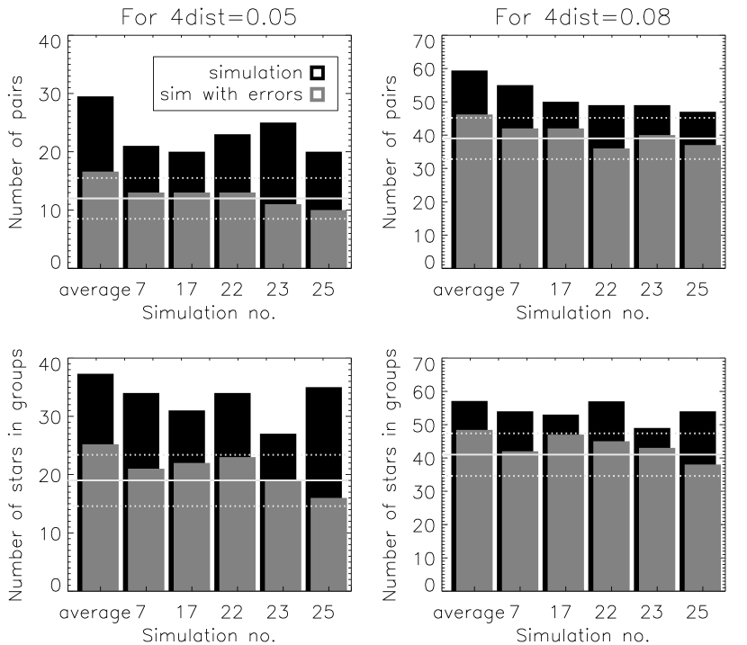
Figure 6.— Top panels show the number of pairs detected with the 4distance method at $4dist\leq 0.05$ and $4dist\leq 0.08$ for the average of 30 “K-giant” simulations constructed with the sampling of the Spaghetti survey and for the five simulated sets out of these simulations that most resemble the Spaghetti data set in terms of the amount of substructure found. The black and gray bars correspond to the results obtained for the simulated subsets before and after (observational) error convolution. The white horizontal line represents the number of pairs found in the Spaghetti data set, the dashed lines show 1$\sigma$ deviation assuming Poissonian statistics. The bottom panels show, for the same simulations, the number of stars associated with substructures according to our algorithm.

This implies that the simulated data sets have a significant fraction of stars originating in narrower streams than in the observed data set. Because these streams are more confined, this substructure is easily picked up by our 4distance method. The fact that nearly all simulated data sets show more substructure especially at $4dist\leq 0.05$ means that the structures we trace in the Milky Way halo are broader.

In the simulations, the average number of stars associated with pairs according to our algorithm is 25%, despite the fact that all of the halo was built by accretion. This points to a fundamental limit in our ability to recover substructure which is due to the rather small sample of stars we have at our disposal. If the number of ‘giants’ in each of our simulated data sets were to be increased to $\sim 1.000$, the $4dist$ method would find on average 76% of the ‘stars’ to be in substructures. Clearly, larger spectroscopic surveys should thus be able to improve significantly on the limits we have set with the Spaghetti project.

4.2. Performance of the 4Distance method

In this section we describe several tests performed using the simulations to test the reliability and determine the strengths and weaknesses of the 4distance method. First, we now check in the simulated data sets whether the substructure found originates from a common parent satellite, i.e., whether all pair members originate in the same progenitor. At $4dist\leq 0.05$ 76% of the pair members in all the simulated data sets do share common parent satellites (this number grows to 87% if we do not take observational errors into account). The number of mismatches is slightly larger when we look at $4dist\leq 0.08$, but still 64% of the pair members at this level share common progenitors. As we increase the numbers of the ‘giants’ per bin in the simulated data sets by a factor of 10 to $\sim 1.000$ in total, 81% of the pair members (convolved with errors) at $4dist\leq 0.05$ do share a common parent satellite. These percentages show that the 4distance works well in the sense that it does not produce many “false positives”: pairs that do not originate from a common progenitor.

To further explore the effectiveness of the 4distance method we have selected five disrupted satellites from our simulations. Their debris streams have different surface brightness and they move on different orbits, with distances to the Sun that range from less than 10 kpc to more than 120 kpc. We use this subset of the simulations to test which of these characteristics determine how well the 4distance method performs as measured by the number of pairs with $4dist\leq 0.05$. For this purpose, we select 15 fields of 5^∘ by 5^∘, three on each stream. The properties of the fields are shown in Figure 7. The number of stars in each field is clearly different, corresponding to a difference in surface brightness. In Figure 8 we plot the number of pairs at $4dist\leq 0.05$ found in each field, as a function of the stars in each field (left panel) and as a function of the average distance of the stars in the selected field (right panel). This figure shows that the average distance has little (if any) bearing on the number of pairs found by the 4distance algorithm. Clearly, the most important factor determining the number of pairs found is the number of giants (i.e., surface brightness) of the stream.

The surface brightness of a stream depends on several factors (see, e.g., Helmi & White 1999, Johnston et al. 2001):

• the orbit (more extended orbits give rise to streams with a lower surface density)

• the initial mass and phase space density of the progenitor system (for a fixed mass, denser systems give rise to streams with higher surface brightness, while at fixed density less massive objects give rise to streams with lower surface density)

• the time since formation of the stream, compared to the orbital period (older accretion events produce lower surface brightness streams by the present day) (see also Johnston et al. 2008).

Therefore the success of the 4distance method depends on all these factors (indirectly) because they all impact the surface brightness of a stream at the present day, but it is only the surface brightness of the stream which affects its ability to recover substructure.

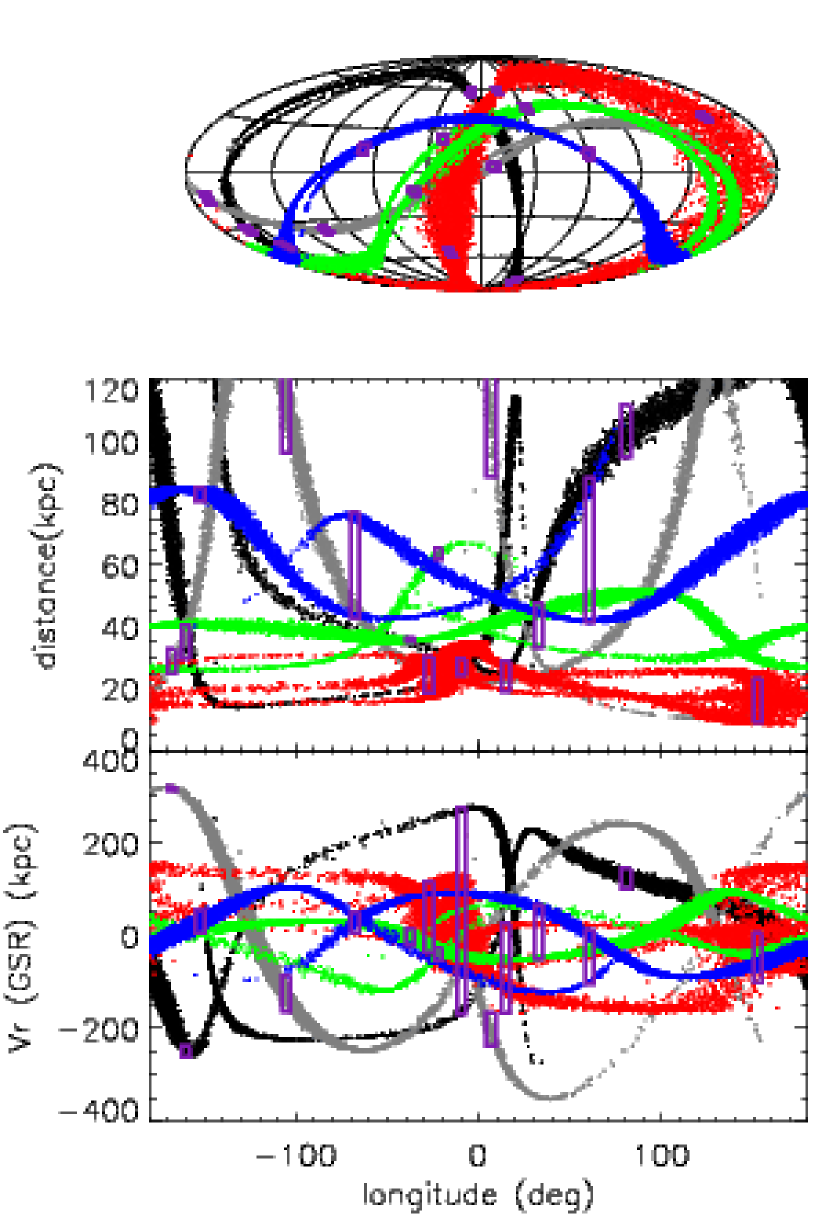
Figure 7.— All ‘giants’ from five simulations of disrupted satellites (in the online version the five satellite streams have different colors) with on top 15 boxes of 5^∘ by 5^∘ (purple in the online version) we selected on the streams. Top panel: the ‘giants’ plotted on the sky in galactic longitude (centred at zero) and galactic latitude. Middle and bottom panel: the same simulations and boxes in galactic longitude vs. distance from the Sun and radial velocity, respectively.

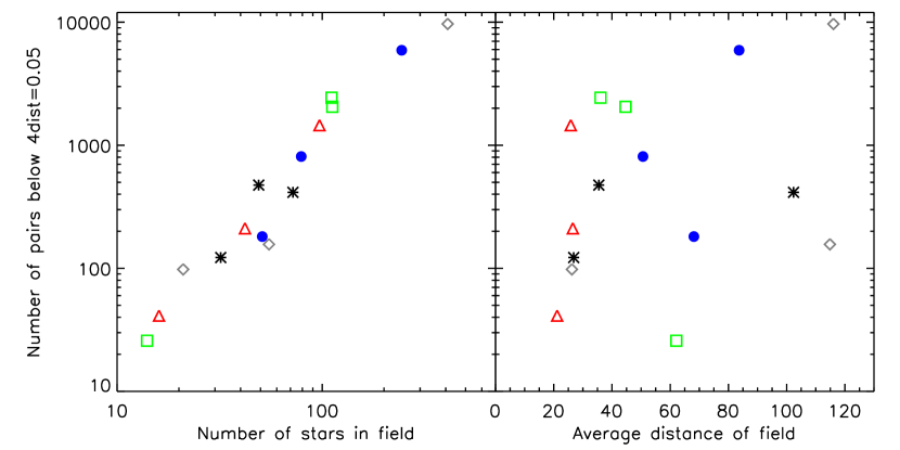
Figure 8.— Left panel: the number of pairs found in each of the 15 fields shown in Figure 7 as a function of the number of ‘giants’ selected in that field. Fields from the same satellite stream have the same symbol (and the same color as in Figure 7 in the online version). The number of giants in the field is directly proportional to the surface brightness of the stream. Right panel: the number of pairs found in each selected field as a function of the average distance of these giants from the Sun.

We use the same subset of five simulations to demonstrate how crucial (radial) velocity information is to identify streams, since this is a key feature of our survey and of ongoing projects such as the SEGUE K-giant survey (Yanny et al. 2009). Although the power of additional velocity information can already be seen in Figure 7, we quantify this advantage here. For this purpose we select a 5^∘ by 5^∘ field which stretches from 2^∘ to 7^∘ in galactic longitude and 35^∘–40^∘ in galactic latitude in Figure 7, and which contains 134 ‘giants’. In this particular field, four different streams cross each other, providing us with an opportunity to demonstrate the value of additional radial velocity information in such cases, which are known to occur in the Milky Way halo as well (e.g., the streams from Sagittarius near the North Galactic Pole).

Subsequently we calculate both the 4distance value for all pairs from the 134 ‘giants’ in this field and also a ‘3distance’ value, omitting the velocity term in Equation 3. Although the absolute values will vary for both methods, we can still make a fair comparison by comparing the most significant pairs in both methods. These are defined as those with the smallest metric values. In Figure 9 we plot the percentage of ‘correct’ pairs (pairs for which the members originate from a common parent satellite) for a fixed number (expressed as a percentage of the total number) of most significant pairs sorted in increasing order of the metric values for each method. From this figure it is very clear that the 4distance method performs much better in selecting correct pairs at small 4distances, whereas the 3distance method is picking up many false positives already for its most significant pairs. For comparison, the $4dist\leq 0.05$ restriction used on the Spaghetti data set in Section 3.1, corresponds to $\sim 10\%$ of the total number of pairs (shown as the vertical dashed line). With the 4distance method, the percentage of correct pairs at this level is over 80%, while without the velocity information one would select roughly 50% false positive pairs. This shows that velocity information is crucial in identifying individual streams, especially because several streams can be overlapping on the sky.

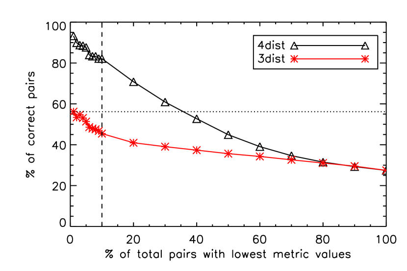
Figure 9.— For the 5^∘ by 5^∘ field taken from Figure 7 around $(l,b)=(5^{\circ},38^{\circ})$ this figure shows the percentage of ‘correct’ pairs found with the 4distance or 3distance method as function of the percentage of the total number of pairs found, sorted by their metric (4distance or 3distance) value. The vertical dashed line therefore indicates the 10% of pairs in the sample which have the lowest metric (3distance or 4distance) value (in this example these are all the pairs with a $4dist$ value of $\leq 0.05$, of which more than 80% are correct). The horizontal dotted line indicates that the percentage of correct pairs when the smallest 1% 3distance values are considered is already less than 60%.

We also tested the possibility to link the found substructures with the 4distance method to larger, more streamlike features using a great circle counts method (Lynden-Bell & Lynden-Bell 1995, Palma et al. 2002). We found however that such an approach is not suitable for our data set because of the pencil-beam character of our survey. The method and discussion of the results can be found in the Appendix. In the next section we explore the performance of the 4distance method in recovering known substructure.

5. Are these substructures new?

Using the 4distance method, we identified one group and seven pairs of stars which are likely to be real substructures in the Milky Way halo. We now explore whether these can be related to other structures previously discovered.

5.1. The Sagittarius Dwarf Galaxy

In Dohm-Palmer et al. (2001), the Spaghetti Collaboration reported a concentration of giant stars which stood well above the expectations of a smooth halo model. In particular, four stars could be matched to a simulation model of the debris from the disrupting Sagittarius spheroidal dwarf galaxy (Helmi & White 2001).

In our examination of the full Spaghetti data set we find this same overdensity to be very prominent: our largest group, with six members. The substructure, at $l=-3.8^{\circ}$ to $l=5.3^{\circ}$, $b=48.6-61.3^{\circ}$ and distances between 48 and 59 kpc, has properties in excellent agreement with the debris predictions of models from Helmi (2004). Several other studies have reported overdensities in this region of the sky and at similar distances (e.g., Yanny et al. 2000, Ivezić et al. 2000, Ibata et al. 2001b, Martínez-Delgado et al. 2001, Vivas et al. 2001, Majewski et al. 2003, Sirko et al. 2004, Belokurov et al. 2006) which have also been associated with debris from Sagittarius. At this region in space several wraps of Sagittarius cross each other, some recently stripped from the satellite and some stripped quite early. This raises the possibility that the stars do not all originate from the same wrap which can explain the spread in metallicities observed. Our method did not find Dohm-Palmer et al. (2001)’s additional proposed structures at distances of 20 and 80 kpc to be significant, because the stars in these structures do not define a tight clump on the sky.

The average metallicity of the giants in group 1, [Fe/H]$\approx-1.7$, is lower than the mean and about $-1.0$ dex lower than is found for stars in the leading arm closer to the main body of the Sagittarius dwarf galaxy (e.g., Monaco et al. 2007, Chou et al. 2007). Because the stars in the outskirts of a galaxy are stripped off first, a metallicity difference between wraps would then reflect a metallicity gradient in the dwarf galaxy itself. Dwarf spheroidal galaxies do in fact often possess metallicity gradients (e.g., Tolstoy et al. 2004). Furthermore, a strong difference in horizontal branch morphology has been detected between the Sagittarius core and a portion of the leading arm of the Sgr stream (Bellazzini et al. 2006). This difference is consistent with the difference in metallicity between the core and the stream stars in our group 1: the metal-richer core has more red horizontal branch stars and the metal-poorer stream has more blue horizontal branch stars.

Also pairs 5, 7, and 8 could be associated with the disrupting dwarf galaxy. Comparison to simulations of Sagittarius by Helmi (2004) shows this is possible if these stars were stripped off early, between 3 and 6 Gyr ago. Pair 5 matches best in a prolate halo. The membership of pairs 7 and 8 is, however, more likely if the galactic halo potential is significantly more oblate than prolate (when the flattening of the potential is $q=0.8$), but we think there is stronger evidence these pairs are linked with the Virgo overdensities and not to Sagittarius debris (see the next section). The group and three pairs and a Sagittarius prolate model are plotted on the sky, in distance and velocity in Figures 10–12.

5.2. The Virgo Substructures

Several overdensities have been discovered toward the constellation of Virgo (Vivas et al. 2001, Newberg et al. 2002, Zinn et al. 2004, Jurić et al. 2008, Duffau et al. 2006, Newberg et al. 2007, Keller et al. 2008). The origin of these features and whether they are all part of the same large structure is still unclear (Newberg et al. 2007). Two substructures (pairs 7 and 8) are near these overdensities on the sky and have distances that agree with those measured for the Virgo overdensities. Also the velocities, although very different for the two pairs, match approximately those reported in the literature.

The same two pairs were also discussed in the previous section as possible matches with older Sagittarius debris. This is not surprising since this debris is close to Virgo on the sky. Newberg et al. (2007) have however convincingly shown on the basis of SDSS photometry that the Virgo overdensities are too low in latitude to be members of the (leading) tidal tail of Sagittarius. Indeed in prolate halo models it is predicted that the Sagittarius stream should not overlap with the Virgo overdensities, as shown in Figure 10.

Figures 10–12 show the location of the overdensities reported in the literature and of the group and pairs we have just identified in a polar plot and in distance and velocity respectively. Our pairs match the known Virgo overdensities, both from SDSS and RR Lyrae surveys, relatively well in sky position, distance and velocity. It is interesting to note that these results suggest that Virgo is not a global ‘smooth’ feature of the Galaxy (see also Xu et al. 2006). Rather it resembles a very complex ‘Spaghetti bowl’, because all the stars observed toward this direction are on kinematic substructures and do not show a smooth Gaussian-like underlying velocity distribution.

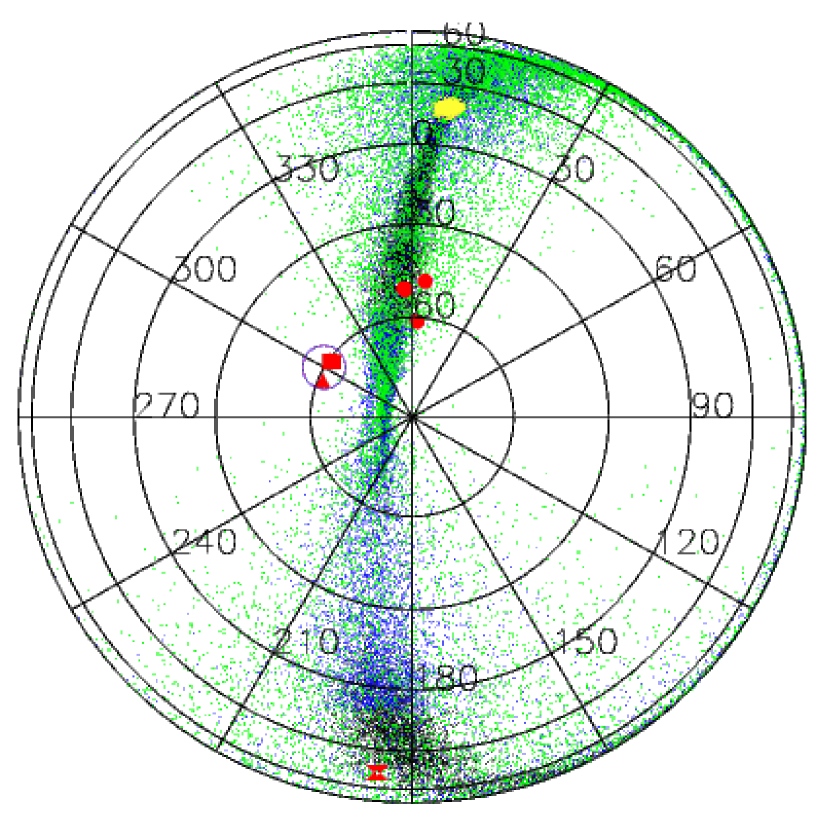
Figure 10.— Polar plot in galactic coordinates (l,b) of the whole sky showing the location of debris from a model of the Sagittarius dwarf galaxy orbiting in a prolate dark halo (q=1.25) potential. The debris is color-coded (in the online version) according to “dynamical age”: stripped off less than 3 Gyr ago (black dots), between 3 and 6 Gyr ago (blue dots), more than 6 Gyr ago (green dots). The main body of the galaxy is shown in yellow. Also overplotted are group 1 and pairs 5, 7, and 8 (red circles, hourglasses, triangles, and squares, respectively) and the approximate region of the overdensity found in SDSS photometry by Newberg et al. (2007) (purple circle).

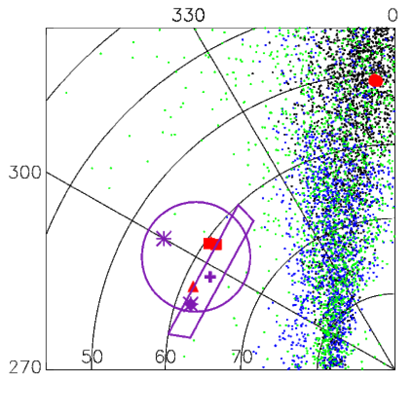
Figure 11.— Zoom-in of Figure 10 onto the Virgo region. The same color coding (in the online version) and symbols are used as in Figure 10. The additional rectangular shape denotes the region of the RR Lyrae overdensity in QUEST (Zinn et al. 2004). A purple diamond shows the position of the Virgo Stellar Stream (Duffau et al. 2006), a purple plus the overdensity S297+63-20.5 in SDSS (Newberg et al. 2002) and the purple asterisks point at two directions in which spectra are obtained with SEGUE (Newberg et al. 2007). One of the SEGUE plates overlaps with the direction of the Virgo Stellar Stream on the sky.

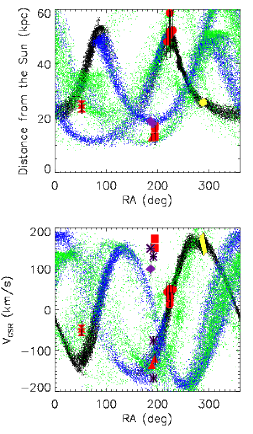
Figure 12.— Distance from the Sun vs. right ascension (top panel) and radial velocity vs. right ascension (bottom panel) for all the structures previously shown in Figures 10 and 11 (same color coding in the online version) with known distances and velocities. The Sagittarius model (blue, green, black, and yellow dots) is not shown as a fit to the Virgo substructures. Newberg et al. (2007) link a Galactic standard of rest velocity of 130 $\pm$ 10 km s^-1 to the S297+63-20.5 overdensity. Other velocities shown here with purple asterisks correspond to subsequent significant moving groups they found in these fields.

5.3. Other matches

There is remarkable similarity between the properties of our pair 3 and of clump 3 from Clewley & Kinman (2006). Adding their BHB stars in that clump to our sample and performing our 4distance measure results in a large group in which contains both our pair 3 and three of their stars from their clump 3.

6. Discussion

Based on the number of stars (101 giants), Spaghetti is a small survey, certainly compared with very extensive survey projects like SDSS. The main aspects that have made the Spaghetti project unique are the high quality of its data, its depth–which has allowed the discovery of giant stars out to $\sim 100$ kpc, and the amount of information for every object: distances with ‘just’ 15% error bars, a thorough luminosity classification, radial velocity information (critical for the identification of substructure) and metallicity measures for every halo giant.

Through our newly defined distance measure, the 4distance, we have been able to trace large substructures in the outer halo of the Milky Way using the Spaghetti data set. We have confidently identified a clump of debris from the disrupting Sagittarius dwarf galaxy as well as other pairs that might be part of Sagittarius’ older debris or are, more likely, associated with Virgo substructures. These results are found to be quite robust under small changes of the group-finding algorithm. We tried several weighting factors as well as different levels of the $4distance$ measure and found that both influence the overall result only marginally.

A method which resembles ours slightly, is the Stellar Pair Technique developed by Clewley & Kinman (2006). This requires pairs to have at most a three-dimensional distance of 2 kpc and a radial velocity difference of $\leq 25$ km s^-1. These choices for the separation are motivated by the suspected characteristics of streams. They do not take into account the varying errors in the observables, nor chance clustering. This is why we deem our method, which by itself selects a clustering scale, more suitable.

We have also tested the 4distance method on Monte Carlo data sets drawn from simulations of disrupted satellites. This analysis shows that when a substructure is identified, 76% of its members share a common physical origin. This further strengthens our conviction that this method is reliable.

While the Spaghetti survey is well suited to find and trace substructures especially far out in the halo, like any red giant survey it has limitations on the surface brightness of the substructures it can detect. For example the Orphan Stream, which has been modeled to originate from a progenitor with a stellar mass of $\sim 7.5\times 10^{5}M_{\odot}$ (Sales et al. 2008), seems to be right on this boundary. While the Spaghetti survey has three fields right where the Orphan Stream reaches its peak surface brightness, we only find two probable candidate members in these fields (Sales et al. 2008). This also means that “pure” red giant surveys may not be able to put any constraints on the low-mass end of the luminosity function of objects accreted very early on, perhaps analogous to the recently discovered ultrafaint satellites (e.g., Simon & Geha 2007). On the other hand, as shown in Figures 7 and 8, the only limiting factor for detection of substructure by our 4distance method seems to be the surface density of the stream. In this sense, the 4distance method is not biased toward accretions of any particular type, with the caveat that the size of the data set will impose a lower limit on the surface brightness of the structures the method will be able to detect.

The main goal of the Spaghetti survey was to establish the amount of substructure in the stellar halo. The analysis we have performed on this data set allows us to quantify this combining kinematics and spatial information, which is a unique approach. In our significant pairs we found 20 giants, which is 20% of all the giants in the Spaghetti data set. Of these 20 giants, 19 were found in the first step of the method, at $4dist\leq 0.05$. From the analysis of random sets we expect about five pairs with on average nine giants in them to be chance matches. This would leave 10 ‘real’ matched giants in the data set. We think this measure is conservative, because both the amount of substructure we found which can be linked to already known substructures, like Sagittarius and Virgo, already indicate a fraction in substructures of $>$10% and the analysis of the pairs found in the simulated data sets also show that a high percentage of all matches might be real. Finally and more importantly, even in the simulated data sets only 25% of the ‘stars’ were in pairs according to our method, despite the fact that the simulated halo was fully composed of streams.

Our limitation is clearly the size of the sample, which means that Poissonian statistics dominate our analysis and estimation of the significance of our results. The comparison to the simulations evidences that we cannot put an upper limit on the total amount of substructure in the halo. Although in our data set we find no more than 20% to be in large substructures well above our detection limit, which would be around the mass of the Orphan Stream progenitor, it is also consistent with the whole outer halo having been built from accreted satellites. Larger spectroscopic surveys will probably be able to improve this significantly. We estimate using our simulations that in samples with 1000 giants the amount of substructure detected by the 4distance method should raise to approximately 76%. It will be important in the context of ongoing and future surveys (e.g., SEGUE, Yanny et al. (2009); SEGUE II, Rockosi et al. (2009); HERMES, Raskin & Van Winckel (2008); and WFMOS, Bassett et al. (2005)) to confirm these estimates using cosmological simulations of stellar halos. We defer this to future work, as well as establishing which is the best strategy to map the halo (e.g., contiguous fields vs. pencil beams) to unravel its assembly history.

We were able to trace the Sagittarius dwarf galaxy and the Virgo overdensity, the only two known large substructures in the part of the sky probed by the Spaghetti survey. However, because the survey has only probed a small number of directions on the sky, it is very well possible that we have missed relatively large substructures at larger distances, or in other directions. It is remarkable however that although $\sim$35% of the fields observed by Spaghetti are outside of the sky coverage of SDSS, only one pair of stars (pair 6) is found in that region. This would suggest that the substructure in the halo is not isotropically distributed on the sky, and therefore is unlikely to be the result of the overlap of a large number of high surface brightness, narrow streams.

Most of our 30 simulated data sets show a larger amount of substructure than found in the Spaghetti survey. On average there is an excess of structure at small scales ($4dist\leq 0.05$). Therefore, although our results are consistent with the whole stellar halo being built by accretion, the characteristic size of the structures found by the Spaghetti survey is larger than what is produced by $10^{7}$M_⊙ satellites. This can be due to earlier accretion, or more massive satellites. Some additional support to this interpretation comes from the fact that the estimated mass for the original Sagittarius galaxy is $\sim$50–100 times the mass of our simulated satellites (Helmi 2004, Law et al. 2005).

7. Conclusions

We have developed a method to measure the amount of substructure in surveys consisting of spatial and radial velocity information for halo stars. When applied to the final data set from the Spaghetti survey, we find one group and seven pairs which contain a total of 20 stars. The most outstanding group, with six members, can confidently be associated with debris from the disrupting Sagittarius dwarf galaxy. Another pair might be associated with older Sagittarius debris. On the basis that the Virgo overdensity is not linked to the Sagittarius leading tail (as demonstrated by Newberg et al. (2007)), two other pairs can be associated with known Virgo overdensities. Simulations in which this works, prefer a prolate halo shape.

The stars in groups and pairs constitute 20% of the Spaghetti data set. Comparison with random sets allows us to derive a very conservative lower limit of 10% of the stars to be truly associated to substructures. Unfortunately, no conclusive upper limit can be given. From comparison with data sets drawn from a simulated halo made entirely of $10^{7}$M_⊙ disrupted satellites we find that the Spaghetti data set marginally supports that the whole stellar halo was built by accretion of such galaxies. The characteristics of the substructure found in the Milky Way halo seem to imply that broad streams dominate our data set. This would suggest early merging and/or relatively heavy progenitors.

Further insights and better constraints may be obtained from deep imaging of the regions around these substructures and from high-resolution spectroscopy of the giant stars listed in Table 2.

Appendix A The Great Circle method

The 4distance method as developed in this work is suitable to look for substructures on small scales; predominantly clumplike structures. On the other hand, we also expect to see a significant amount of large-scale streamlike structures, particularly in the outer halo. To search for these streams, we adopt a great circle method (Lynden-Bell & Lynden-Bell 1995, Palma et al. 2002). The main assumption underlying this method is that accreted debris from a satellite orbits in a plane containing both the current position of the satellite and the Galactic center, whose intersection with the celestial sphere is a great circle on the sky. This assumption requires a spherical potential, a requirement which holds relatively well in the outer halo.

All objects on the same orbit share also the same ‘orbital pole’, defined by the direction of their angular momentum. For each star, the direction of the orbital pole is perpendicular to the vector drawn from the Galactic center to the star’s current position. An indication of possible linkage in dynamical history in our data set would therefore be to find several objects on a great circle associated with (so perpendicular to) a common orbital pole. Due to the pencil-beam character of the Spaghetti survey, however, it is not feasible to perform an investigation based on just the sky positions (and thus great circles) of the stars alone, like for instance a pole-count analysis as performed in Ibata et al. (2001c) using C stars from the APM survey.

A.1. Specific Energy and Angular Momentum

The specific energy of the star’s motion is given by:

$$E=\text@frac{1}{2}v_{gal}^{2}+\text@frac{1}{2}h^{2}r^{-2}+\Psi$$ (A1)

Although the exact values of the angular momentum, $h$, and the specific energy, $E$, of each star are unknown, we may assume that they are constant for debris from the same parent satellite (Lynden-Bell & Lynden-Bell 1995). The distance from the Galactic center, $r$, is available and a first approximation to the radial velocity as seen from the Galactic Center ($v_{gal}$) is given by the measured line-of-sight velocity after correction for the motion of the local standard of rest ($v_{GSR}$). Furthermore, we may assume a functional form for the Galactic potential, $\Psi$. Rewriting Equation A1 as:

$$E_{r}=E-\text@frac{1}{2}h^{2}r^{-2}\approx\text@frac{1}{2}v_{GSR}^{2}+\Psi$$ (A2)

we obtain a first approximation for $E_{r}$. Because $E$ and $h$ are constants, we expect to see a linear dependence in an $E_{r}$ vs. $r^{-2}$ plot for all the stars originating from a common parent satellite.

The results for all the stars that are farther out than 10 kpc in our data set are shown in the upper panel of Figure 13. The gray solid curve indicates the contribution to $E_{r}$ of the Galactic potential for these stars, obtained using the model of Johnston, Spergel and Hernquist (1995). The figure shows that most of the stars follow the trend dictated by the overall potential. The bottom panel of Figure 13 shows the same diagram for a random set, constructed as described in Section 3.1. Clearly there is no significant difference between the two panels. This leads us to conclude that this method is not suitable for our data set. Although by eye it appears possible to fit straight lines through many points in the top panel, this is also the case for the bottom panel, which is devoid of substructure by construction. Another concerns are the extensive error bars in the data set.

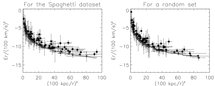
Figure 13.— Left panel shows the $E_{r}$ vs. $r^{-2}$ diagram for all stars farther out than 10 kpc in the Spaghetti data set. The error bars account for distance and velocity uncertainties. The solid gray line represents the contribution of the Galactic potential to $E_{r}$ for these stars. The right panel shows a similar plot, but for a random set instead of the Spaghetti data set.

A.2. Combination of both requirements

Because of the limitations discussed above, we will only use the great circle method in a complementary fashion to the 4distance method in order to determine whether any of the previously found substructures can, on the basis of sky position, energy and angular momentum considerations, be linked to other structures located on the sky.

We measure the average position of every group or pair shown in Table 2 which is farther out than 10 kpc from the Galactic center. In the search for the angular momentum pole each group or pair is thus treated as one object. We bin the sky in 2.5^∘ by 2.5^∘ areas where every sky element represents an orbital pole direction. Subsequently we count the number of objects found on a 10^∘ wide band following the great circle of each orbital pole direction. If three or more objects are found on one great circle, a least-square method is used to define the likelihood that the corresponding members of these objects in the $E_{r}$ vs. $r^{-2}$ diagram can be fitted by a straight line. We require a high probability (Q=0.99) on the straight line fit and a small error on the slope and intersection with the y-axis ($\leq 10\%$). If such a fit can be obtained, all the stars found in the groups or pairs associated with one orbital pole direction are considered to be possible debris from the same parent satellite. For every match the largest possible association is considered, provided that at least three of the objects were initially more than 10^∘ apart on the sky.

When applying this method to the previously found groups and pairs within the Spaghetti data set, of which five are beyond 10 kpc, we find one association of groups and pairs that have a possible dynamical linkage, including group 1 and pairs 5, 7 and 8. Although in the paper, we argued that the stars in these group and pairs in fact might be unrelated in dynamical origin, belonging to separate Virgo and Sagittarius substructures (see Section 5.2), their linkage by this method is not surprising since they do lie closely to a single great circle on the sky.

A.3. Substructure in the simulated data sets: great circles

We now focus on the combined great circle method, and apply it to the five simulated data sets, described in Section 4, which show the closest resemblance to our data set (numbers 7, 17, 22, 23 and 25). The results for these simulated data sets are given in Table 3. The number of associations of linked groups and pairs with one great circle on the sky and of which their ‘giants’ were on a straight line in the $E_{r}$ vs. $r^{-2}$ diagram are given in the second column. The third column shows the fractions of associations that are ‘correct’. We define an association of groups or pairs to be ‘correct’ if at least two of its groups or pairs are from a common progenitor and if more than 50% of the stars within the association originate from this common parent satellite.

In total only 12.5% of all associations in these five simulated data sets are called ‘correct’ using our criteria. None of the associations links purely stars from one common satellite. This poor result is partly due to the fact that almost none of the simulated data sets possess enough groups or pairs (as defined by the 4distance method) from the same progenitor. In our implementation of the great circle method, we can link only three or more groups or pairs, while almost never three or more groups or pairs from the same object are found in our simulated data sets. Only in simulated data set 17, more than two groups were found that stem from a common progenitor. Still, the great circle method matches a substantial number of unrelated groups and pairs together. In three of the five examined simulated data sets, all groups and pairs were found in at least one association. This result shows that great care must be exercised when using the great circle method on data sets which are as small, have a nonuniform sky distribution and as “large” distance errors as the Spaghetti data set.

Table 3Properties of the associations of groups and pairs found using the combined great circle method on the data set and several simulated data sets.

Data Set	# Associations	Fraction of
		correct associations
Spaghetti	1	?/1
Sim7	7	0/7
Sim17	9	2/9
Sim22	2	0/2
Sim23	3	1/3
Sim25	3	0/3

A.4. Conservation of total energy and angular momentum and the role of errors

We can use our simulations also to understand how well the assumption of conservation of angular momentum holds, and what the effects of errors (observational, but also due to projection effects) are. In Figure 14 we plot a subset of five streams from the final output of the simulations (the same subset of streams as was used in Section 4.2). Shown are the distance from the Sun vs. galactic longitude (upper panel), the theoretical $E_{r}$ vs. $r^{-2}$ diagram for the simulations themselves, using no errors and computed using the true radial velocities from the Galactic center (middle panel) and the ‘observed’ $E_{r}$ vs. $r^{-2}$ diagram obtained by convolving the simulations with ‘observational’ errors (bottom panel). As expected satellites on orbits which come close to the Galactic center conserve their total angular momentum (and angular momentum pole) less well as is shown in the middle panel. However, the observational errors and our limited leverage on the radial velocity (i.e., as measured from the Sun) are mostly responsible for destroying the tight correlations in the $E_{r}$ vs. $r^{-2}$ diagram between particles from a common satellite.

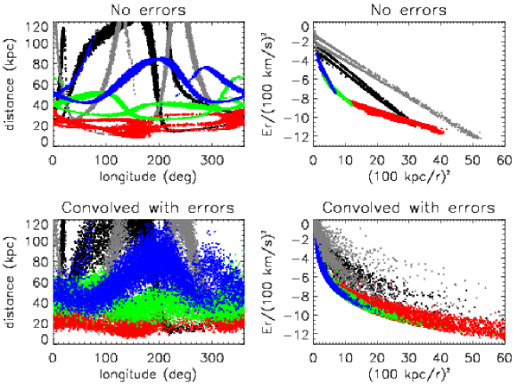
Figure 14.— All ‘giants’ from simulations of five disrupted satellites. The left panels show the streams in galactic longitude vs. distance. In the right panels the stream ‘giants’ are plotted using the same color coding in an $E_{r}$ vs. $r^{-2}$ diagram. However, the top panels use the original simulated streams and the true value for $E_{r}$, while in the bottom panels the ‘giants’ properties are convolved with ‘observational’ errors and the line-of-sight velocities, transformed to the Galactic standard of rest, are used as a proxy to the radial velocity of a star.

References

- Adelman-McCarthy et al. (2007) Adelman-McCarthy, J. K., et al. 2007, ApJS, 172, 634
- Bassett et al. (2005) Bassett, B. A., Nichol, B., & Eisenstein, D. J. 2005, Astron. Geophys., 46, 050000
- Bell et al. (2008) Bell, E. F., et al. 2008, ApJ, 680, 295
- Bellazzini et al. (2006) Bellazzini, M., Newberg, H. J., Correnti, M., Ferraro, F. R., & Monaco, L. 2006, A&A, 457, L21
- Belokurov et al. (2006) Belokurov, V., et al. 2006, ApJ, 642, L137
- Belokurov et al. (2007a) Belokurov, V., et al. 2007a, ApJ, 657, L89
- Belokurov et al. (2007b) Belokurov, V., et al. 2007b, ApJ, 658, 337
- Bullock & Johnston (2005) Bullock, J. S., & Johnston, K. V. 2005, ApJ, 635, 931
- Chou et al. (2007) Chou, M.-Y., et al. 2007, ApJ, 670, 346
- Clewley & Kinman (2006) Clewley, L., & Kinman, T. D. 2006, MNRAS, 371, L11
- Dehnen & Binney (1998) Dehnen, W., & Binney, J. J. 1998, MNRAS, 298, 387
- de Jong et al. (2007) de Jong, R. S., et al. 2007, IAU Symposium, 241, 503
- de Jong et al. (2008) de Jong, R. S., Radburn-Smith, D. J., & Sick, J. N. 2008, Astronomical Society of the Pacific Conference Series, 396, 187
- Dohm-Palmer et al. (2000) Dohm-Palmer, R. C., Mateo, M., Olszewski, E., Morrison, H., Harding, P., Freeman, K. C., & Norris, J. 2000, AJ, 120, 2496
- Dohm-Palmer et al. (2001) Dohm-Palmer, R. C., et al. 2001, ApJ, 555, L37
- Duffau et al. (2006) Duffau, S., Zinn, R., Vivas, A. K., Carraro, G., Méndez, R. A., Winnick, R., & Gallart, C. 2006, ApJ, 636, L97
- Grillmair & Dionatos (2006) Grillmair, C. J., & Dionatos, O. 2006, ApJ, 643, L17
- Harding et al. (2001) Harding, P., Morrison, H. L., Olszewski, E. W., Arabadjis, J., Mateo, M., Dohm-Palmer, R. C., Freeman, K. C., & Norris, J. E. 2001, AJ, 122, 1397
- Helmi (2004) Helmi, A. 2004, MNRAS, 351, 643
- Helmi & White (1999) Helmi, A., & White, S. D. M. 1999, MNRAS, 307, 495
- Helmi & White (2001) Helmi, A., & White, S. D. M. 2001, MNRAS, 323, 529
- Ibata et al. (1994) Ibata, R. A., Gilmore, G., & Irwin, M. J. 1994, Nature, 370, 194
- Ibata et al. (2001a) Ibata, R., Irwin, M., Lewis, G., Ferguson, A. M. N., & Tanvir, N. 2001a, Nature, 412, 49
- Ibata et al. (2003) Ibata, R. A., Irwin, M. J., Lewis, G. F., Ferguson, A. M. N., & Tanvir, N. 2003, MNRAS, 340, L21
- Ibata et al. (2001b) Ibata, R., Irwin, M., Lewis, G. F., & Stolte, A. 2001b, ApJ, 547, L133
- Ibata et al. (2001c) Ibata, R., Lewis, G. F., Irwin, M., Totten, E., & Quinn, T. 2001c, ApJ, 551, 294
- Ibata et al. (2007) Ibata, R., Martin, N. F., Irwin, M., Chapman, S., Ferguson, A. M. N., Lewis, G. F., & McConnachie, A. W. 2007, ApJ, 671, 1591
- Ivezić et al. (2000) Ivezić, Ž., et al. 2000, AJ, 120, 963
- Johnston et al. (2008) Johnston, K. V., Bullock, J. S., Sharma, S., Font, A., Robertson, B. E., & Leitner, S. N. 2008, ApJ, 689, 936
- Johnston et al. (1996) Johnston, K. V., Hernquist, L., & Bolte, M. 1996, ApJ, 465, 278
- Johnston et al. (2001) Johnston, K. V., Sackett, P. D., & Bullock, J. S. 2001, ApJ, 557, 137
- Johnston et al. (1995) Johnston, K. V., Spergel, D. N., & Hernquist, L. 1995, ApJ, 451, 598
- Jurić et al. (2008) Jurić, M., et al. 2008, ApJ, 673, 864
- Keller et al. (2008) Keller, S. C., Murphy, S., Prior, S., DaCosta, G., & Schmidt, B. 2008, ApJ, 678, 851
- Law et al. (2005) Law, D. R., Johnston, K. V., & Majewski, S. R. 2005, ApJ, 619, 807
- Lynden-Bell & Lynden-Bell (1995) Lynden-Bell, D., & Lynden-Bell, R. M. 1995, MNRAS, 275, 429
- Majewski et al. (2003) Majewski, S. R., Skrutskie, M. F., Weinberg, M. D., & Ostheimer, J. C. 2003, ApJ, 599, 1082
- Martin et al. (2004) Martin, N. F., Ibata, R. A., Bellazzini, M., Irwin, M. J., Lewis, G. F., & Dehnen, W. 2004, MNRAS, 348, 12
- Martínez-Delgado et al. (2001) Martínez-Delgado, D., Aparicio, A., Gómez-Flechoso, M. Á., & Carrera, R. 2001, ApJ, 549, L199
- Martínez-Delgado et al. (2008) Martínez-Delgado, D., Peñarrubia, J., Gabany, R. J., Trujillo, I., Majewski, S. R., & Pohlen, M. 2008, ApJ, 689, 184
- Martínez-Delgado et al. (2009) Martínez-Delgado, D., Pohlen, M., Gabany, R. J., Majewski, S. R., Peñarrubia, J., & Palma, C. 2009, ApJ, 692, 955
- Mathewson et al. (1974) Mathewson, D. S., Cleary, M. N., & Murray, J. D. 1974, ApJ, 190, 291
- Monaco et al. (2007) Monaco, L., Bellazzini, M., Bonifacio, P., Buzzoni, A., Ferraro, F. R., Marconi, G., Sbordone, L., & Zaggia, S. 2007, A&A, 464, 201
- Moody et al. (2003) Moody, R., Schmidt, B., Alcock, C., Goldader, J., Axelrod, T., Cook, K. H., & Marshall, S. 2003, Earth Moon and Planets, 92, 125
- Morrison et al. (2000) Morrison, H. L., Mateo, M., Olszewski, E. W., Harding, P., Dohm-Palmer, R. C., Freeman, K. C., Norris, J. E., & Morita, M. 2000, AJ, 119, 2254
- Morrison et al. (2001) Morrison, H. L., Olszewski, E. W., Mateo, M., Norris, J. E., Harding, P., Dohm-Palmer, R. C., & Freeman, K. C. 2001, AJ, 121, 283
- Morrison et al. (2003) Morrison, H. L., et al. 2003, AJ, 125, 2502
- Newberg et al. (2007) Newberg, H. J., Yanny, B., Cole, N., Beers, T. C., Re Fiorentin, P., Schneider, D. P., & Wilhelm, R. 2007, ApJ, 668, 221
- Newberg et al. (2002) Newberg, H. J., et al. 2002, ApJ, 569, 245
- Palma et al. (2002) Palma, C., Majewski, S. R., & Johnston, K. V. 2002, ApJ, 564, 736
- Peñarrubia et al. (2005) Peñarrubia, J., et al. 2005, ApJ, 626, 128
- Raskin & Van Winckel (2008) Raskin, G., & Van Winckel, H. 2008, Proc. SPIE, 7014, 70145D
- Rockosi et al. (2009) Rockosi, C., Beers, T. C., Majewski, S., Schiavon, R., Eisenstein, D., & with input from the SDSS-III Collaboration 2009, arXiv:0902.3484
- Sales et al. (2008) Sales, L. V., et al. 2008, MNRAS, 389, 1391
- Shang et al. (1998) Shang, Z., et al. 1998, ApJ, 504, L23
- Simon & Geha (2007) Simon, J. D., & Geha, M. 2007, ApJ, 670, 313
- Sirko et al. (2004) Sirko, E., et al. 2004, AJ, 127, 899
- Skrutskie et al. (2006) Skrutskie, M. F., et al. 2006, AJ, 131, 1163
- Tolstoy et al. (2004) Tolstoy, E., et al. 2004, ApJ, 617, L119
- Vivas et al. (2001) Vivas, A. K., et al. 2001, ApJ, 554, L33
- Vivas et al. (2004) Vivas, A. K., et al. 2004, AJ, 127, 1158
- Xu et al. (2006) Xu, Y., Deng, L. C., & Hu, J. Y. 2006, MNRAS, 368, 1811
- Yanny et al. (2009) Yanny, B., et al. 2009, AJ, 137, 4377
- Yanny et al. (2000) Yanny, B., et al. 2000, ApJ, 540, 825
- Zinn et al. (2004) Zinn, R., Vivas, A. K., Gallart, C., & Winnick, R. 2004, Satell. Tidal Streams, 327, 92