A Search for Occultations of Bright Stars by Small Kuiper Belt Objects using Megacam on the MMT

Abstract

We conducted a search for occultations of bright stars by Kuiper Belt Objects (KBOs) to estimate the density of sub-km KBOs in the sky. We report here the first results of this occultation survey of the outer solar system conducted in June 2007 and June/July 2008 at the MMT Observatory using Megacam, the large MMT optical imager. We used Megacam in a novel shutterless continuous–readout mode to achieve high precision photometry at 200 Hz. We present an analysis of $220$ star hours at signal-to-noise ratio of 25 or greater. The survey efficiency is greater than 10% for occultations by KBOs of diameter $d\geq 0.7~{}\mathrm{km}$, and we report no detections in our dataset. We set a new 95% confidence level upper limit for the surface density $\Sigma_{N}(d)$ of KBOs larger than 1 km: $\Sigma_{N}(d\geq 1~{}\mathrm{km})~{}\leq~{}2.0\times 10^{8}~{}\mathrm{deg}^{-2}$, and for KBOs larger than 0.7 km $\Sigma_{N}(d\geq 0.7~{}\mathrm{km})~{}\leq~{}4.8\times 10^{8}~{}\mathrm{deg}^{-2}$.

1. Introduction

The size distribution of objects in the Kuiper Belt is believed to be shaped by competitive processes of collisional agglomeration and disruption. The details of the structure of the Kuiper Belt size distribution can reveal information on the internal structure of the Kuiper Belt Objects (KBOs), the history of planet migration (Kenyon & Bromley, 2004; Pan & Sari, 2005), and the gas history in the Solar System (Kenyon & Bromley, 2009). Large objects in the Kuiper Belt (diameter $d\geq 30~{}\mathrm{km}$) can be observed directly in reflected sunlight. The luminosity distribution for objects larger than $~{}100~{}\mathrm{km}$ is well described by a single power-law cumulative luminosity distribution $\Sigma_{N}(<R)=10^{\alpha(R-R_{0})}$, where $\Sigma_{N}(<R)$ is the number of KBOs brighter than magnitude R per degree in the sky on the ecliptic plane, with an index $\alpha\sim 0.7$ and $R_{0}\sim 23$ (Fraser et al., 2008; Fuentes & Holman, 2008). This, under the assumption of 4% constant albedo, translates into a power-law size distribution $n(d)\propto d^{-q}$ with power index $q\sim 4.5$. For these objects the size distribution reflects the history of agglomeration.

There is strong evidence for a break in the slope of the distribution at fainter magnitudes (smaller KBO sizes). Constraints on the extrapolation of a single power law to magnitude greater than $R\sim 35$ were placed by Kenyon & Windhorst (2001), who invoked Olbers’s Paradox applied to the Zodiacal Background, and by Stern & McKinnon (2000), who derived a slope for the distribution of small KBOs of $q\approx 3$ on the basis of the cratering on Triton as observed by Voyager 2. A further hint of a break in the size distribution of KBOs is offered by the better–probed size distribution of Jupiter Family Comets (JFCs, Tancredi et al. 2006, and references therein). These objects are likely injected into their current orbits from the Kuiper Belt or the scattered disk (Volk & Malhotra, 2008), and it is argued that their size distribution would be preserved during this process. The size distribution of JFCs is well represented by a shallow slope: $q~{}=~{}2.7$ in the diameter range $1-10~{}\mathrm{km}$. Future Microwave Background surveys may also allow the setting of constraints on the mass, distance, and size distribution of Outer Solar System (OSS) objects (Babich et al., 2007).

Bernstein et al. (2004) conducted a deep Hubble Space Telescope survey with the Advanced Camera for Surveys which led to the detection of three KBOs of magnitude $R>26.5$; an extrapolation of the bright end power-law would have predicted a factor of about $25$ more detections for this survey. This reveals that a break in the power law distribution must occur at magnitude brighter than $R~{}=~{}28.5$ ($\mathrm{d}\sim 20~{}\mathrm{km}$). This work remains the state of the art in deep direct surveys of the OSS, with a completeness of 50% at magnitude $R=28.5$. More recently Fuentes et al. (2008) and Fraser & Kavelaars (2009) detected more KBOs in the $R\leq 27$ region of the size spectrum and better constrained the slope of the bright end of the power law and the location of the break, $R~{}\sim~{}25$ ($d\sim 50-100~{}\mathrm{km}$, Fuentes et al. 2008, Fraser & Kavelaars 2009).

KBOs smaller than about $30~{}\mathrm{km}$ in diameter still elude direct observations. Occultation surveys are the only observational method presently expected to be able to detect such small objects in the Kuiper Belt. These surveys monitor background stars awaiting the serendipitous alignment of KBOs with the stars. The transit of a KBO along the line of sight briefly modifies the observed flux of the target star. At the distance of the Kuiper Belt ($\sim 40~{}\mathrm{AU}$) the size of the objects of interest is close to the Fresnel scale for visible light: this causes such occultation events to be diffraction dominated phenomena. The Fresnel scale is defined as $F=\sqrt{\lambda D/2}$ (Born & Wolf, 1980; Roques et al., 1987), where $D$ is the distance to the occulter and $\lambda$ the wavelength at which the occultation is observed. In our survey the bandpass of the observation is centered near $\lambda~{}=~{}500~{}\mathrm{nm}$ and, at distance $D~{}\approx~{}40~{}\mathrm{AU}$, $F\approx 1.2~{}\mathrm{km}$. Any occultation caused by objects in the Kuiper Belt of a few kilometers in diameter or smaller will exhibit prominent diffraction effects. A diffraction pattern, characterized by an alternation of bright and dark fringes centered on the KBO, translates into a modulated lightcurve during the transit of the KBO along the line of sight. A unique feature, showing a series of wiggles, and generally a reduction in flux, is imprinted in the time series of the star (Roques & Moncuquet, 2000; Nihei et al., 2007, see Figure 1).

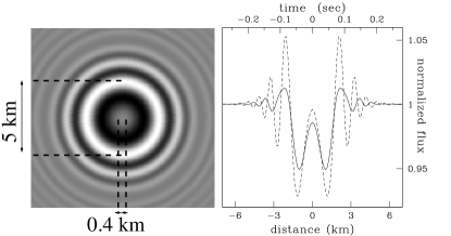
Figure 1.— A simulated diffraction pattern (left panel) generated by a spherical $d~{}=~{}1~{}\mathrm{km}$ KBO occulting a magnitude 12 F0V star. The MMT/Megacam system bandpass (Sloan r’ filter and camera quantum efficiency) is assumed. The size of the KBO and the size of the Airy ring – a measure of the cross section of the event – are shown for comparison. The right panel shows the diffraction signature of the event (assuming central crossing: impact parameter $b~{}=~{}0$) as a function of the distance to the point of closest approach (bottom scale). The top scale shows the time-line of the event assuming an observation conducted at opposition (relative velocity $v_{\mathrm{rel}}~{}\approx~{}25~{}\mathrm{km~{}s}^{-1}$). The occultation is sampled at 200 Hz (dashed line), and at 30 Hz, the effective sampling rate after taking PSF effects into account (solid line, see Section 4).

The overall flux reduction is dominated by the size of the KBO, while the duration of the event depends upon the relative velocity $v_{\mathrm{rel}}$ and the size of the diffraction pattern $H$. We define $H$ as the diameter of the first Airy ring, which it is limited by the Fresnel scale for sub-km KBOs and by the size of the object for large KBOs as follows (Nihei et al., 2007):

$$H\approx\left[\left(2~{}\sqrt{3}F\right)^{3\over 2}+d^{3\over 2}\right]^{{2\over 3}}~{}+~{}D\theta_{\star},$$ (1)

where the additional $d\theta_{\star}$ term accounts for the finite angular size of the star. When observing at opposition the relative velocity $v_{\mathrm{rel}}$ of an object orbiting the sun at $40~{}\mathrm{AU}$ is about $25~{}\mathrm{km~{}s^{-1}}$ and the typical duration of an occultation by sub-km KBOs is about $0.2$ seconds.

Occultation surveys were first proposed by Bailey (1976), but only recently have results been reported. Chang et al. (2007) conducted a search for KBO occultations in the archival RXTE X-ray observations of Scorpius-X1. They reported a surprisingly high rate of occultation–like phenomena: dips in the lightcurves compatible with occultations by objects between $10$ and $200~{}\mathrm{m}$ in diameter. Jones et al. (2008) showed that most of the dips in the Sco-X1 lightcurves may be attributed to artificial effects of the response of the RXTE photo-multiplier after high energy events, such as strong cosmic ray showers. In the 90 minutes of RXTE data analyzed only $12$ of the original $58$ candidates cannot be ruled out as artifacts, but are hard to confirm as events (Jones et al., 2008; Chang et al., 2007; Liu et al., 2008). New RXTE/PCA data of Sco X-1 provided a less constraining upper limit to the size distribution of KBOs (Liu et al., 2008).

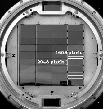
Figure 2.— Megacam focal plane (McLeod et al., 2006). A thick rectangle outlines a single CCD in the 9x4 CCDs mosaic. Two halves of each CCD (thin rectangles) are read into two separate amplifiers; each amplifier generates a separate output image in our observational mode. The $x$ and $y$ axis, as they would appear in a resulting image, are also shown.

Several groups have conducted occultation surveys in the optical regime. Roques et al. (2006) and Bickerton et al. (2008) independently observed narrow fields at $45~{}\mathrm{Hz}$ and $40~{}\mathrm{Hz}$, respectively, with frame transfer cameras. Such cameras allowed them to obtain high signal-to-noise ratio (SNR) fast photometry on two stars simultaneously. Both surveys expect a very low event rate due to the limited number of stars and the limited exposure, and neither survey has claimed any detection of objects in the Kuiper Belt at this time. An upper limit for KBOs with $d\geq 1~{}\mathrm{km}$ was derived by Bickerton et al. (2008) by combining the non-detection result of the surveys of Chang et al. (2007), Roques et al. (2006), and Bickerton et al. (2008). TAOS (Taiwanese American Occultation Survey) is a dedicated automated multi-telescope survey (Lehner et al., 2009) that has observed a set of fields comprising $\sim 500$ target stars for over 3 years, collecting over 150,000 star hours. TAOS reported no detections but placed the strongest upper limit to date to the surface density of small KBOs (Zhang et al., 2008). TAOS observes at slower cadence (4 or 5 Hz) and has a relatively low sensitivity ($\mathrm{SNR}\approx 40$ at magnitude $R=12$). For these reasons TAOS is only marginally sensitive to sub-km objects (with recovery efficiency $\epsilon_{\mathrm{TAOS}}\approx 0.3\%$ at 700 m and $\epsilon_{\mathrm{TAOS}}\approx 0.03\%$ at 500 m).

The survey we report here was conducted using Megacam (McLeod et al., 2006, Figure 2) at the 6.5 m MMT Observatory at Mount Hopkins, Arizona. The use of Megacam in continuous–readout mode (see Section  2) on a field of view of $24^{\prime}\times 24^{\prime}$ allowed us to monitor over 100 stars at 200 Hz over the course of two observational campaigns conducted in June 2007 and June-July 2008. Our survey is sensitive to occultations of OSS objects $d\sim 700~{}\mathrm{m}$ or larger and we report no detections in 220 star hours. Our MMT survey is designed to be complementary to TAOS and to reach smaller size limits, and unlike TAOS it would allow us to estimate the size of a detected occulting KBO. We expect further work on adaptive photometry and de-trending to significantly improve our sensitivity, perhaps allowing us to detect KBOs as small as $d\geq 300~{}\mathrm{m}$. We discuss the improvements we are developing on this analysis in Section 7. The preliminary analysis we present here allows us to derive upper limits for objects $d\geq 700~{}\mathrm{m}$.

In the next section we describe the novel observational mode adopted for this survey. In Section 3 we describe the data acquired and analyzed for this paper. Details of the data extraction and reduction, which required custom packages, are addressed in the same section. Section 4 describes the characteristics of the noise of our current datasets, and our noise mitigation approach. Section 5 describes the detection algorithm. In Section 6 we derive our upper limit to the density of KBOs. We also compare in detail the achievements of our survey to those of previous surveys. We draw our conclusions and outline future work in Section 7.

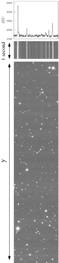
Figure 3.— Conventional stare mode image (one half of a CCD) of one of our fields (bottom panel). A series of rows from continuous–readout mode (center panel) from the same CCD and field, where the rows are stacked together in a single image. The flux profile of the central row of this segment of continuous–readout data is plotted in the top panel.

2. Fast Photometry with a Large telescope: The Continuous–Readout Mode

Figure 4.— Top: power spectrum of one of our lightcurves before and after de-trending the lightcurve to remove noise (see Section 3.1.2). Bottom: power spectrum of the occultation time–series for a 1 km KBO at 40 AU occulting a F0V $~{}V=~{}12$ star.

Achieving sub-second photometric sampling is a challenge in optical astronomy. CCD Cameras can perform fast photometric observations by reading out small sub-images, limiting the observations to very small portions of the sky (e.g., Marsh & Dhillon 2006). This is the approach adopted by Roques et al. (2006), and Bickerton et al. (2008), who observed two stars at one time. Due to the rarity of occultation events, however, one would want to maximize the number of targets and the total exposure to increase the number of detections. TAOS achieves sub-second photometric observation on up to 500 targets with the zipper mode readout technique (Lehner et al., 2009), but they sample at $\leq~{}5~{}\mathrm{Hz}$ rate. Our continuous–readout technique allows us to observe the entire field of view of the camera at $200~{}\mathrm{Hz}$.

Megacam, the MMT optical imager, is a mosaic camera comprising thirty-six CCDs – each with an array of $2048\times 4608$ pixels – with a $24^{\prime}\times 24^{\prime}$ field of view (Figure 2). The standard readout speed of each CCD is 0.005 sec/row with $2\times 2$ binning. For this survey, we operated the camera in shutterless continuous–readout mode; that is, we kept the shutter open while scrolling and reading the charges at the standard readout speed, tracking the sky at the sidereal rate. Each star is represented in each row that is read out of the camera, and the flux from a star in a row represents a photometric measurement of that star sampled at 200 Hz. Stacking each read row into a single image each star time–series forms a streak along the readout axis ($y\mathrm{-axis}$). A small portion of our data is shown in Figure 3.

In this observational mode the flux from the sky background is added continuously as the charge is transferred from one end of the CCD to the other, so the sky is exposed $2304\times 0.005~{}=~{}11.52~{}\mathrm{sec}$ for every 0.005 sec integration on each star image (where 2304 is the effective number of rows in each $2\times 2$ binned CCD). In this mode the photon limited SNR is typically $\sim 180$ for an $r^{\prime}$ magnitude 10 star.

When observing multiple targets simultaneously one can notice that the star lightcurves are affected by common fluctuations, or trends, due for example to weather patterns (Kim et al., 2008, and references therein). In our observational mode, however, additional flux variations are caused by wind-induced resonant oscillations of the telescope. While the image motion along the $x$ axis of the focal plane (transverse to the readout direction) can be resolved (see Section 3.1.1), the image motion parallel to the direction of the CCD readout induces an effective variation in the exposure time of a star for a given row. These fluctuations are common to all stars in the field (with possible position dependencies) and therefore, in principle, they are completely removable. We discuss the de-trending of our data in Section 3.1.2. Other sources of noise that affect continuous-readout mode data are discussed in Section 4. The typical duration of a set of contiguous data was 10–15 minutes (after which the data load on the buffer would become prohibitive). For each amplifier, a single FITS file is created wherein all of the rows read out during a data run are stored as a single image. For a typical run each FITS output image contains $100\mathrm{K}$ to $130\mathrm{K}$ rows, corresponding to about 150–200 Mb of data.

3. Data

Table 1Parameters of the observed fields

RA	Dec	$\lambda$	$\varepsilon$ range
		(deg)	(deg)
$17^{\mathrm{h}}00^{\mathrm{m}}00^{\mathrm{s}}$	$-21^{\circ}15^{\prime}00^{\prime\prime}$	1.5	174–160
$17^{\mathrm{h}}15^{\mathrm{m}}00^{\mathrm{s}}$	$-20^{\circ}15^{\prime}00^{\prime\prime}$	2.8	176–163
$18^{\mathrm{h}}00^{\mathrm{m}}00^{\mathrm{s}}$	$-21^{\circ}15^{\prime}00^{\prime\prime}$	2.2	171–173
$18^{\mathrm{h}}00^{\mathrm{m}}00^{\mathrm{s}}$	$-21^{\circ}30^{\prime}00^{\prime\prime}$	1.9	171–173
$18^{\mathrm{h}}00^{\mathrm{m}}00^{\mathrm{s}}$	$-21^{\circ}45^{\prime}00^{\prime\prime}$	1.7	172–173
$19^{\mathrm{h}}00^{\mathrm{m}}00^{\mathrm{s}}$	$-22^{\circ}00^{\prime}00^{\prime\prime}$	0.7	158–172

We selected observing fields within $2.8^{\circ}$ of the ecliptic plane, where the concentration of KBOs is highest (Brown, 2001). In order to maximize the number of targets we selected our fields at the intersection of the ecliptic and galactic planes ($\mathrm{RA}~{}\sim 19^{\mathrm{h}}00^{\mathrm{m}}00^{\mathrm{s}}$, $~{}\mathrm{Dec}~{}\sim-21^{o}00^{\prime}00^{\prime\prime}$). We conducted our observations in June-July, when our fields were near opposition (elongation angle $\varepsilon~{}=~{}180^{\circ}$) and the relative velocity of the KBOs is highest (Roques et al., 1987; Nihei et al., 2007; Bickerton et al., 2009), thus maximizing the event rate per target star. Pointing information for our fields is summarized in Table 1. The RA and Dec of each observed field are listed together with the ecliptic latitude ($\lambda$) and a maximum range of elongation angles at which the filed might have been observed.

We also observed control fields. These were chosen on the galactic plane at a high ecliptic latitude; we expect a negligible rate of occultations by KBOs in these fields. These data allow us to assess our false positive rate. Since we report no detections the analysis of these fields is not discussed further in this paper. All of our observations were conducted in Sloan $r^{\prime}$ filter (Smith et al., 2002). A set of about $7$ hours on target fields was collected in 5 half nights in June 2007 and a similar number of hours was collected on control fields. A set of about $7$ hours on target fields and about $6$ hours on control fields was collected in 7 half nights in June-July 2008. Out of the 2007 dataset 100.61 star hours at $\mathrm{SNR}\geq 25$ are considered in this paper. From the 2008 dataset we use here 118.93 star hours. Information on our dataset is summarized in Table 2. The minimum signal-to-noise ratio of 25, is chosen arbitrarily: 25 is the minimum $\mathrm{SNR}$ of the surveys of Roques et al. (2006) and Bickerton et al. (2008). A SNR 25 limits our sensitivity to fluctuations greater than $4\%$. An occultation of a magnitude 12 F0V star by a KBO of $d=400~{}\mathrm{m}$ diameter would produce a $4\%$ effect. Our efficiency tests, however, revealed our sensitivity rapidly drops below 10% for objects smaller than $d=700~{}\mathrm{m}$, due to residual non-Gaussianity in our time–series photometric data. We discuss this in Section 4.

Table 2Data set parameters.

Start Date	2007 June 6
End Date	2007 June 10
Exposure at SN$\geq 25$	100.61 star-hours
Number of lightcurves with SN$\geq 25$	990
Number of Photometric Measurements	$7.2\times 10^{7}$
Start Date	2008 June 27
End Date	2008 July 1
Exposure at SNR$\geq 25$	118.93 star-hours
Number of lightcurves with SNR$\geq 25$	527
Number of Photometric Measurements	$8.5\times 10^{7}$

3.1. Data extraction and reduction

3.1.1 Extraction

Custom algorithms have been developed for the data extraction and reduction. For each field a preliminary stare mode (conventional) image is collected before each series of high-speed runs. At the beginning of our analysis the stare mode image is analyzed using SExtractor (Bertin & Arnouts, 1996) to generate a catalog of bright sources. This catalog is used to identify the initial position and brightness of each star in the focal pane. In order to analyze the continuous readout data, we first determine the sky background for each CCD and each row. To do so we calculate the mean of the flux counts in each row after removing the measurements that are three $\sigma$’s or more from the mean ($3\sigma$-clipping) iteratively until the mean converges. This removes most of the pixels in the row containing flux from resolved stars. Next, a subset of stars that are bright and isolated is selected from the stare–mode catalog and used to determine the $x$-displacement of the focal plane. The focal plane is split into two halves, $9\times 2$ chips each, that are analyzed separately. We select eight stars, two near each of the four corners of each half-focal plane. This allows us to characterize the global motion of the targets even in the presence of small rotational modes or spatial dependency (see Section 4). For each star ($\star$), and at each time–stamp (t), we calculate $\mu_{\star}(t)$ and $\sigma_{\star}(t)$, respectively the centroid offset from the original position and the standard deviation of the star image, assuming a Gaussian profile. Note that, for a given time-stamp, flux from different stars will appear on different rows due to the $y$-positions of the stars on the focal plane. A 1-D Gaussian

$$F_{\star}~{}=~{}I_{\star}~{}\exp\left(-\frac{(x-\mu_{\star}(t))^{2}}{2\sigma_{\star}^{2}(t)}\right)~{}+~{}I_{bg}$$ (2)

(where $F_{\star}$ is the total star flux, $I_{\star}$ the flux at the peak and $I_{\mathrm{bg}}$ the sky) is fit for each of the eight stars to each row of the star–streak. Thus the $x$-displacement $\bar{\mu}(t)$ for all the stars in the field at time–stamp $t$ is estimated to be the weighted average of the star displacements:

$$\bar{\mu}(t)~{}=~{}\frac{\sum\limits_{\star=1}^{8}\omega_{\star}(\mu_{\star}(t)-\mu_{\star}(t_{0}))}{\sum\limits_{\star=1}^{8}\omega_{\star}},$$ (3)

where $\mu_{\star}(t_{0})$ is the star initial $x$-position and $\omega_{\star}$ is the weight used for that star.

In order to weight our average we use the correlation of the entire $x$–displacement time–series ${\mathbf{\mu}_{\star}}$ with respect to the rest of the star set:

$$\omega{(i,j)} = \frac{1}{T}\sum_{t=0}^{T}\frac{(\mu_{i}(t)-\left<\mu_{i}\right>)(\mu_{j}(t)-\left<\mu_{j}\right>)}{s_{i}^{2}(t)~{}s_{j}^{2}(t)},$$ (4)

$$\omega_{\star} = \frac{1}{7}\sum_{j\neq\star}\omega(\star,j);$$ (5)

where $s^{2}$ is the variance of the displacement throughout the duration $T$ of the time–series. The weight $\omega_{\star}$ is the square of the Pearson’s correlation coefficient (Rice, 2001, pag. 406), a measure of the correlation of the displacement time–series for one star with the other seven. All star lightcurves in the field are then extracted by aperture photometry adjusting time–stamp by time–stamp the center of the aperture according to the $x$-motion derived in this stage, and with a fixed aperture size which is proportional to the average FWHM in the run.

3.1.2 De-trending

The lightcurves thus extracted show evident semi–periodic, quasi–sinusoidal flux variations that can be associated with oscillatory modes of the telescope in the $y$ direction. In particular, a Fourier analysis generally reveals two strong modes, roughly consistent among runs, one with period near $0.04$ seconds and the other near $0.5$ seconds. Fourier spectra for one of our lightcurves, before and after processing it, are shown in Figure 4 (top). Because these fluctuations affect the whole CCD plane, they are common to all stars and can be removed to achieve greater photometric precision. We now want to identify and remove these trends from our lightcurves, a process that we call de-trending.

Figure 5.— Image motion and PSF over time: mean of the $x$ displacements for eight bright isolated stars, at the four corners of the half-focal plane for two data runs (top left and right panels). PSF width from the Gaussian fit averaged over the same set of stars (bottom left and right). On the left we used the same run used to generate Figure 8. The arrow points to the displacement feature marked in Figure 8. On the right the $x$-displacement and the PSF width for another run, with the first 0.5 seconds shown on the left at higher time resolution. Note how in the second run the $x$-displacements are less prominent (note the different $y$ scale) but the amplitude of the variability of the PSF is larger.

The general algorithm we used for de-trending is described in Kim et al. (2008). The method takes advantage of the correlation among lightcurves to extract and remove common features. Since we can identify distinct semi–periodic modes we de-trend high and low frequencies separately (typically $\nu>10\mathrm{Hz}$ and $\nu<10\mathrm{Hz}$).

We first smooth the lightcurves, to remove all but the frequencies that we want to de-trend, by applying a low–pass or high–pass filter. We then select a subset of $N_{\tau}$ template lightcurves ($f_{\tau}$) that show the highest correlation in the lightcurve features. $N_{\tau}$ is typically about 15. A master trend lightcurve $\tau$ is generated as the weighted average of the normalized template lightcurves:

$$\tau(t)=\frac{1}{N_{\tau}}~{}\frac{\sum\limits_{j=1}^{N_{\tau}}\sigma^{2}(f_{\tau,j})~{}f_{\tau,j}(t)/\langle f_{\tau,j}\rangle}{\sum\limits_{j=1}^{N_{\tau}}\sigma^{2}(f_{\tau,j})}$$ (6)

where the notation $\langle f_{\tau,j}\rangle$ denotes the mean flux of $f_{\tau,j}(t)$ over the duration $T$ of the lightcurve, and the weight $\sigma^{2}(f_{\tau,j})$ is the variance of the lightcurve in time; $\tau(t)$ has mean value of unity and it represents the correlated fluctuations in all lightcurves.

The main trend is physically associated with an over-under exposure phenomenon due to global image motion along the $y$ axis, which causes the effective exposure time to vary (see Section 2), therefore scaling the flux. In order to remove these common trends we divide point by point the flux of each original lightcurve $f$ by the trend master lightcurve. To improve the de-trending effectiveness we allow a free multiplicative factor $A_{f}$ (a scaling factor) for each lightcurve as follows:

$$f_{\mathrm{d},A_{f}}(t)~{}=~{}f(t)\left[\left(\frac{1}{\tau(t)}-1\right)A_{f}~{}+~{}1\right];$$ (7)

$f_{\mathrm{d},A_{f}}$ is the de-trended lightcurve.

We optimize our de-trending by selecting $A_{f}$ to minimize the variance of the de-trended lightcurve $f_{\mathrm{d}}$ with respect to $f_{\mathrm{c}}~{}=~{}f-f_{\mathrm{s}}+\langle f_{s}\rangle$, which is the original lightcurve cleaned of the frequency to be de-trended. We apply a high–pass (low–pass) filter to $f$ to obtain $f_{\mathrm{s}}$ if we want to de-trend the low (high) frequencies. $A_{f}$ is then optimized by setting:

$$\frac{\partial}{\partial A_{f}}\sum_{t=1}^{T}\left(f_{\mathrm{d},A_{f}}(t)~{}-~{}\langle f_{\mathrm{c}}\rangle\right)^{2}=0,$$ (8)

which minimizes the second moment of the de-trended lightcurve with respect to $f_{\mathrm{c}}$. The optimal value of $A_{f}$ can be calculated analytically.

We set no constraints on $A_{f}$, and for all of our runs the optimal values of $A_{f}$ proved to be close to 1 (which is what we expect in the presence of global trends) except for pathological cases where the flux of the star was buried in noise and the raw and detrended SNR were extremely low. These lightcurves would not pass SNR cuts and were never considered in any of our analysis.

Examples of the results obtained by our de-trending algorithm are displayed in Figures 6 and 7. In Figure 6 the top two panels show lightcurves for two independent sources in our field, and the bottom two panels show the same lightcurves after de-trending. Note that the top star is $\sim 2.5$ magnitudes brighter than the other and this is reflected in the lower SNR of the fainter source (bottom panel). Figure 7 shows one of our lightcurve before (top) and after de-trending (bottom). The raw lightcurve is implanted with an occultation by a $d~{}=~{}1~{}\mathrm{km}$ KBO occulting a $V=9$ F0V star. The diffraction feature is completely lost in the trends and becomes evident only after de-trending. In the bottom panel we show the lightcurve detrended without allowing for the optimization factor $A_{f}$ at the top (plotted at the top at an arbitrary offset) and with optimization factor $A_{f}~{}=~{}1.15$ for the low frequencies and $A_{f}~{}=~{}1.05$ for the high frequencies, shown at the bottom. The introduction of an optimization factor improves the SNR of the de-trended lightcurve from $\mathrm{SNR}~{}=~{}30.0$ to $\mathrm{SNR}~{}=~{}30.7$. For this particular run improvements of up to 7% in SNR were achieved by optimizing the detrending.

Note that, while we used smoothed versions of our lightcurves to identify the trends and to optimize the de-trending, we do not smooth or filter our lightcurves to improve the SNR, thus preserving all intrinsic features (including potential occultations). Figure 4 shows the power spectrum of one of our lightcurves before and after de-trending it (top). The power spectrum of an occultation time-series generated by a 1 km KBO occulting a F0V star of magnitude $V~{}=~{}12$ is shown in the bottom panel. Our de-trending greatly reduced the power at all frequencies: the cumulative power for this particular lightcurve at frequencies $\nu\leq 40~{}\mathrm{Hz}$ is suppressed by a factor of 40. Because the oscillations are not perfectly correlated among our stars (see Section 4) some residual power is visible. Smoothing however would would significantly reduce the strength of the occultation features, that show power at all frequencies $\nu<20~{}\mathrm{Hz}$.

Figure 6.— Lightcurves of two independent stars in one of our fields. The left-hand plots show a 0.5-second chunk of the time series; the following 4-seconds are shown on the right at a lower time resolution. The top two panels show the lightcurves before detrending. Common modes are visible at multiple time scales. The bottom two panels show the lightcurves after detrending. The top lightcurve is the same used in Figure 4

4. Residual noise in the time-series

Figure 7.— Raw lightcurve on which the occultation signature of a 1 km KBO occulting a magnitude $V~{}=~{}9$ F0V star has been implanted (top) and the same lightcurve after detrending (bottom). In the bottom panel the top lightcurve is detrended without optimization (plotted at the top at an arbitrary offset) and the bottom lightcurve is detrended with optimization factor $A_{f}~{}=~{}1.15$ for the low frequencies and $1.05$ for the high frequencies.

With a SNR $\gtrsim 25$ we can detect fluctuations of a few–percent. In an 0.005 sec exposure the flux for a magnitude $r^{\prime}=14$ star observed by Megacam is about $10^{3}~{}e^{-}$, which after taking into account the contribution to the noise of the background should lead to a Poisson limited SNR of about $25$. While we were able to remove a large portion of the noise that originally affected our data, we typically cannot reach the Poisson-limit. We have identified five possible sources of noise in our data:

• Contamination by nearby sources. Overlap of stars along the $x$ axis (perpendicular to the read-out direction) within a chip, causes reciprocal contamination in our readout mode and some of the stars in our fields are therefore compromised and excluded from our analysis. Furthermore, oscillations of the images along the $x$ axis causes the relative distance between the star–streaks to change, which causes occasional merging. Note that while these oscillations are simultaneous in time domain, they do not occur in the same row in the recorded image. In each row the star images of two objects that are at a different $y$ position on the CCD plane will not belong to the same time-stamp, therefore the oscillations – while simultaneous – will show a $y$ offset. This is shown in Figure 8. The merging of streaks causes artificially high counts. Aperture photometry with a fixed aperture does not address this issue properly and fitting photometry on individual streaks is a computationally expensive, inefficient method which is also unstable in the presence of multiple sources close to each other.

• Unresolved sources. Sources that are too faint to be visible in our 0.005 sec exposures generate a diffuse background. For the data in Figure 3 the sky level calculated as the $3\sigma\mathrm{-clipped}$ mean of the row counts is 140.5 ADUs. The stare mode image sky level was 48 ADUs for a 5 sec exposure, which would lead to a prediction of 110 ADUs for our $0.005\times 2304$ sec effective continuous–readout exposure. The discrepancy is due to the presence of unresolved streaks associated with faint stars across the field. Summing all the counts in the stare mode image and rescaling by the exposure time of each row we get a number very close to the sum of all counts in a row of continuous-readout data. This contamination introduces extra Poisson noise, but more importantly it introduces non-Poissonian noise as well, since the unresolved sources are affected by the same trends the bright stars display. Our data shows evidence of off–phase correlation that might be induced by unresolved sources.

• Positional dependency in the motion and trends. While we treat all of the stars in the field as an ensemble that moves in a solid fashion along the $x$ and $y$ axes, the image motion might also have a rotational component. This would lead to position dependencies in the motion that are not accounted for by our aperture centering algorithm. We have not seen evidence of dependency on the distance to the center of the focal plane in either motion or trends, but we cannot exclude that occasional rotational modes of the telescope would occur. Differential image motion and flux fluctuations might also be induced by atmospheric seeing. Both of these effects might cause the star–streak to move out of the photometric aperture leading to artificially low counts. The aperture size must be chosen to be such that errors due to contamination by nearby sources and errors due to streaks exiting the aperture are simultaneously minimized. Furthermore in the presence of thin clouds, variations in the transparency might generate trends that would affect different sources at different times as the clouds move across the image. Positional dependencies or variations in transparency might contribute to the off–phase correlation of our data.

• Scintillation. Young’s scaling law (Young 1967, Gilliland et al. 1993, Dravins et al. 1998),

  $$\sigma_{I}~{}=~{}\frac{0.09A^{-2/3}(\sec Z)^{1.75}exp(-\frac{h}{h_{0}})}{\sqrt{2~{}\Delta t}},$$ (9)

  describes the error in flux intensity $I$ due to the low–frequency component of scintillation, with $\sigma=\left(\Delta I/I\right)$ and where $A$ is the telescope aperture (in cm), $Z$ the angle from zenith, $h$ is the height of the turbulence layer, the scaling factor $h_{0}=8000~{}\mathrm{m}$, and $\Delta T$ the integration time. Competing effects are in place in our survey: the large aperture mitigating the noise, and the low air mass contributing to signal degradation. Note however that this relation holds for integration time on scales of seconds or longer. When including the effects of high–frequency scintillation the dependency on the aperture is expected to be steeper:

  $$\sigma_{I}^{2}\propto A^{-7/3}(\sec Z)^{3}\int_{0}^{\infty}C_{n}^{2}(h)h^{2}dh,$$ (10)

  where $C_{n}$ is the refraction coefficient for the turbulent layer (see Dravins et al. 1997 and references therein).

  Using the above equations and representative data from La Palma (Dravins et al., 1998) we estimate that the noise contribution from scintillation is $\sigma_{I}<0.01$, i.e., not the dominant source of residual noise. As compared to the other occultation surveys the term associated to the telescope aperture in the SNR variance ($A^{-7/6}$) is a factor 20 lower than the same factor for the TAOS survey, 4.5 times lower than the same factor for Bickerton et al. (2008) and 1.4 than for the Roques et al. (2006) survey.

• Convolution of the time series with finite PSF. The finite size of the PSF (typically two to three pixels, although it occasionally was as large as seven) causes consecutive measurements to be correlated. This effect is not a source of noise per se, but it changes the spectral characteristics of the noise. The scale of this phenomenon shows up in an autocorrelation analysis with high power at a lag of about seven pixels. This is effectively a kernel convolution of our time series that smoothes the signal, including possible occultation signals, so that while we sample the images at 200 Hz we would expect an occultation signature to be effectively sampled at $\approx 30~{}\mathrm{Hz}$ (see Section 5). Note that this is close to, but slightly short of, the critical Nyquist sampling for occultations dominated by diffraction (Bickerton et al., 2009).

While we achieved significant noise reduction with our detrending, our SNR is typically a factor of two to three lower than the Poisson–limit. Our noise is characterized by high kurtosis, which is indicative of non–Gaussianity. Residual low frequency fluctuations (about 100 points period) are still noticeable in many of our time series (see Figure 6). Possible improvements are discussed in Section 7.

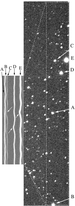
Figure 8.— A stare mode image (right) read out from a single amplifier and a corresponding $\sim 10$ second chunk of high frequency data (left). A few bright stars and the corresponding streaks are indicated by letters. White arrows in the left panel point to a distinctive synchronous displacement feature in the data, visible clearly in three of the streaks, in order to focus the reader’s attention to the non-parallelism of simultaneous features in our data, which is due to offset in the original $y$ position.

Figure 9.— Efficiency plotted against the number of unidentified candidates (mostly false positives). Each line represents a different window size $w$, and each point represents the value of the efficiency at threshold $\theta~{}=$ 0.08, 0.10, 0.15, 0.20, 0.30, the number of false positives monotonically grows with decreasing $\theta$ (larger values of $\theta$ on the left). All lines (all $w$ values) show a plateau at different thresholds.

5. Search for events and efficiency

5.1. Detection algorithm

The signature of an occultation, sampled at any rate $\gtrsim 20~{}\mathrm{Hz}$, is very distinctive: it shows several fluctuations prior to the Airy ring peak, then a deep trough and possibly a Poisson spot feature, followed by a second Airy ring rise and more fluctuations (see Figure 1). The prominence of these features depends upon the magnitude and spectral type of the background star, which together determine the angular size, as well as the size and the sphericity of the occulter, distance to the occulter, and impact parameter (Nihei et al., 2007).

One possible approach to detecting occultations in our lightcurves is to take advantage of this peculiar shape, for example using correlation of templates, as in Bickerton et al. (2008). Given the size of our dataset, however, we chose to utilize a search algorithm general enough to capture any fluctuation of some significance, but which requires less computational power. We scan our time series for any fluctuation lasting longer than a duration $w$, and on average greater than a threshold $\theta$ from the local mean, which is calculated over a window $W$ of 300 data points surrounding $w$. Windows $w$ of 11, 21, 31, 41 and 61 points were considered, in combination with thresholds of 0.10, 0.15, 0.20, 0.30. We define the local intensity $I_{\mathrm{l}}(i)$ as the ratio of the flux in the local window $w$ and in the surrounding window $W$. If the flux in $w$ is suppressed by more than our threshold $\theta$ from the local mean (mean over $W$),

$$I_{\mathrm{l}}(i)~{}=~{}\frac{\displaystyle\sum\limits_{j=i-w/2}^{i+w/2}f_{j}/w}{\displaystyle\sum\limits_{j=i+W/2}^{i+W/2}f_{j}/W}\leq 1~{}-~{}\theta,$$ (11)

then $w$ is considered as a candidate. This is similar to the Equivalent Width algorithm, which is used in spectral analysis, and for rare event searches by Roques et al. (2006) and Wang et al. (2009). Overlapping candidates are then removed and the center of the window $w$ that displayed the largest deviation is selected as a single candidate event. Note that this algorithm would in most cases trigger two separate events for the two halves of an occultation on opposite sides of the Poisson spot (Figure 1). These cases are later automatically recognized and accounted for as a single event. Different choices of $w$ and $\theta$ will produce different detection efficiency and false positive rate. We select an optimized subset of combinations of $w$ and $\theta$ to be used for our event detection. This optimization is described in the next section.

5.2. Efficiency

We test the efficiency of our search by implanting simulated occultations in our raw lightcurves. By using our true dataset instead of generating synthetic data we do not introduce any assumptions about the nature of our time series. We run the implanted lightcurves through the same pipeline as the original lightcurves: de-trending them and searching for significant deviations from the mean flux. In order to achieve better sampling of our efficiency the entire dataset was implanted with one occultation per lightcurve at each KBO size we tested: $d=0.5,0.6,0.7,0.8,0.9,1.0,1.3,2.0,3.0~{}\mathrm{km}$, and the efficiency was assessed for each size separately. The finite PSF width of the star induces correlations among consecutive time stamps. Given the typical PSF size in our data (see Figure 5) measurements are considered independent if separated by more than about seven pixels. Therefore, to modulate the original time series by the occultation signal we multiply the star flux by a synthetic occultation lightcurve sampled at $30~{}\mathrm{Hz}$.

For the purpose of our efficiency simulations we assume all objects are at 40 AU, since we expect our occultations to be within the Kuiper Belt. There is little difference in the diffraction feature between 35 and 50 AU. The differences in spectral power between the star types do not impact the occultation features as observed by our system, so we simulate all of our occultations assuming an F0V type star. The angular size of the star affects the shape of the occultation by smoothing the diffraction features. It is therefore important to properly sample the angular size space. We find that, given the objects in our fields, imposing a flat prior to the magnitude distribution between $V~{}=~{}8$ and $V~{}=~{}11$ adequately samples our angular size range. The flat prior slightly overestimates the average cross section $H$ of the events, but this effect is more than compensated by the loss in efficiency due to the fact that, for stars with larger angular sizes, the occultation signal is smoothed out as the diffraction pattern is averaged over the surface of the star, making the event harder to detect (Nihei et al., 2007). Overall our estimate of our detection rate is conservative.

To characterize our efficiency we implant occultations at random impact parameters $b\in[0,H(d)/2]$. However, we first want to choose the most appropriate window size and threshold combinations, and for that we implant occultations by $d=1~{}\mathrm{km}$ KBOs in the reduced impact parameter space $b~{}\in~{}[0,~{}0.3\cdot H(d)]$. This set of modified lightcurves is used to optimize our parameters to maximize our efficiency and minimize the number of false positives simultaneously. Although our generic detection approach can reach high efficiency (nearly $100\%$ for $1~{}\mathrm{km}$ KBOs at zero impact parameter), it also produces a large number of candidates, most of which are expected to be false positives. The combination of $w$ and $\theta$ values generated efficiencies ranging between 94% (at $w$=11 and $\theta$ = 0.1) and 0 (at $w$=61 and $\theta$ = 0.3) and the number of candidates ranged between 0 and over 1000. Figure 9 shows the behavior of the efficiency as a function of number of candidates. Different window sizes are represented by different lines and the different thresholds are marked by the points along each line. Typically, after a rapid increase in efficiency with the decreasing threshold, the efficiency stabilizes, while the number of candidates keeps growing: we want to choose our parameters near this point, where the efficiency is highest and any less stringent choice would only increase the number of our false positives. We select combinations of $w$ and $\theta$ that yield both an efficiency $>50\%$ and a ratio of efficiency to candidates $<0.5$. The following are the accepted windows-threshold combinations: ($w$, $\theta$) = (21, 0.15), (31, 0.20), and (11, 0.25). Events found in any run with these selection parameters were considered as candidates. We reached an overall efficiency of 82% at $d=1~{}\mathrm{km}$ for lightcurves implanted with synthetic occultations at varying impact parameters between 0 and $H/2$.

The efficiency of our search is summarized in the top panel of Figure 10, as a function of KBO size. We also plot the corresponding effective solid angle $\Omega_{\textrm{e}}(d)$, defined as:

$$\Omega_{\textrm{e}}(d)=\sum_{*}\frac{H(d,\theta_{*})}{D}~{}\frac{v_{\mathrm{rel}}}{D}~{}T_{*}~{}\epsilon(d,~{}\theta_{\star}),$$ (12)

where $H(d,\theta_{*})$ is the cross section of the event, which depends on both the diameter of the KBO and the star angular size as indicated by $\theta_{*}$; $v_{\mathrm{rel}}$ is the relative velocity of the KBO, which depends on the elongation angle which is close to opposition for all of our observations; $D$ is the distance to the occulter (assumed to be $D=40~{}\mathrm{AU}$), $T_{*}$ the exposure for the star target (duration of the lightcurve), and $\epsilon(d,~{}\theta_{\star})$ the recovery efficiency for that diameter: $\epsilon(d,~{}\theta_{\star})~{}=~{}1$ if the implanted event was recovered, 0 otherwise. The sum is carried out over all of our lightcurves with $SNR\geq 25$. $\Omega_{\textrm{e}}(d)$ represents the equivalent sky coverage of our survey for targets at diameter $d$, accounting for a partial efficiency. The center panel of Figure 10 shows the effective solid angle as a function of diameter. The bottom panel shows the effective solid angle multiplied by bracketing slopes for the size distribution: $d^{-4}$ and $d^{-2}$, and it indicates the survey expects to see the largest number of detections near $d~{}=~{}700~{}\mathrm{m}$.

Figure 10.— Efficiency of our survey as a function of KBO diameter (top). The central panel shows the effective solid angle of our survey and the bottom panel the effective solid angle multiplied $d^{-2}$ and $d^{-4}$.

5.3. Rejection of false positives

At this stage we have more than a thousand candidates. However, most of the false positives can be removed in an automated fashion: we reject fluctuations that appear simultaneously in more than one lightcurve; those are most likely due to local weather or atmospheric patterns that were not corrected in the de-trending phase because they only affected a subset of lightcurves, and can be ruled out as serendipitous occultations. We also reject any fluctuation that does not have the right combination of depth and width. We empirically investigate the relationship between the depth and the width of an occultation by a KBO, as it is seen by our system, taking advantage of our simulations. To define the depth and width of the events we fit synthetic occultation lightcurves with inverted top-hat functions with parameters $\Delta$ (depth) and $\Gamma$ (width). Figure 11 shows the best fit values $\Delta$ and the $\Gamma$ for occultations simulated in the diameter range $d=0.1~{}\mathrm{km}$ to $d=3.0~{}\mathrm{km}$, impact parameters $b=0$ to $H/2$ and magnitude range 8 to 11 for F0V stars (the same set that we used for our implantation with additional occultations from objects $d<0.5~{}\mathrm{km}$). The shaded region represents the area of this phase space where at least one occultation was best fit by parameter values $\Delta$ and $\Gamma$ (and the intensity of the shade reflects the frequency of $\Delta-\Gamma$ best fits). We can automatically reject events outside the dashed polygon as incompatible with $d\leq 3.0~{}\mathrm{km}$ KBO occultations. We are not sensitive to events shallower than a 10% flux drop.

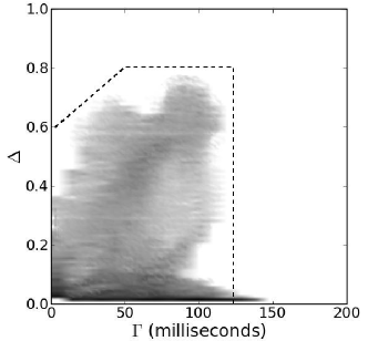
Figure 11.— Phase space plot showing the regions of the flux decrease–duration space occupied by occultations by KBOs of diameter 0.1 to 3 km, as observed through the MMT/Megacam system bandpass. We simulated occultations from KBOs in the size regime 0.1–3.0 km, and we fit the occultations with an inverted top-hat function with parameters $\Delta$ and $\Gamma$. The intensity of the gray scale reflects the number of simulated occultations with best fit value $\Delta$ and $\Gamma$: white areas are void of occultations.

At this point the absolute number of candidates is small ($25$). The remaining candidates are inspected visually (using DS9, Joye & Mandel 2003), and the lightcurves are extracted with a different photometric method (based on IRAF). All remaining candidates prove to be artifacts, mostly due to photometry. No candidates are left after this elimination process.

Figure 12.— Upper limits to the surface density of KBOs. Left panel. The dashed line is the best fit to the Bernstein et al. (2004) survey, extrapolated to $d=0.01\mathrm{km}$. Three data-points reported by Bernstein et al. (2004) are plotted (HST, the faintest data from direct observations). The straight line is the TAOS upper limit to the slope of the small size end size distribution: $q~{}<~{}4.6$ (Zhang et al., 2008). The result by Bickerton et al. (2008) is shown as an empty circle (BKW) as well as the X-ray result (Jones et al., 2008, RXTE). The upper limits set by our survey at $d~{}=~{}1~{}\mathrm{km}$ and $d~{}=~{}0.7~{}\mathrm{km}$ are shown as filled circles. The region relevant to our limit, enclosed in the square, is magnified on the right hand panel. Right panel. Upper limits to the surface density of KBOs, zooming in the 0.2–6 km region of the size spectrum where our survey can place limits. Symbols and labels are the same as for the left panel. The lower limits for JFC precursor populations are also shown (Levison & Duncan, 1997; Morbidelli, 1997; Volk & Malhotra, 2008).

6. Upper limit to the size distribution of KBOs and scientific interpretation

We now compare our limit to the size distribution of KBOs to that of Bickerton et al. (2008). Bickerton et al. (2008) derived an upper limit to the surface density of KBOs of diameter $d\geq 1~{}\mathrm{km}$. They considered the data obtained by their own survey together with the data published by Roques et al. (2006) and Chang et al. (2007), assuming 100% efficiency for each survey at $1~{}\mathrm{km}$, and obtaining a total effective coverage $\Omega_{\textrm{e}}=5.4\times 10^{-10}~{}\mathrm{deg}^{2}$. The cross section $H$ used to calculate $\Omega_{\textrm{e}}$ is set to validate the 100% efficiency assumption on a survey by survey basis. Our survey adds $7.0\times 10^{-9}~{}\mathrm{deg}^{2}$ to the collective $\Omega_{\textrm{e}}$, allowing us to derive a limit over an order of magnitude stronger than the limit set by Bickerton et al. (2008). Thus we set a comprehensive 95% confidence level upper limit on the surface density of $d\geq 1~{}\mathrm{km}$ KBOs at 40 AUs of $\Sigma_{N}(d\geq 1~{}\mathrm{km})~{}\sim~{}2.0\times 10^{8}~{}\mathrm{deg}^{-2}$.

We can also derive a new upper limit for objects as small as $700~{}\mathrm{m}$, where our efficiency is $\epsilon~{}(~{}d~{}=~{}700~{}\mathrm{m})~{}\sim~{}10\%$. We can set a 95% confidence upper limit of $\Sigma_{N}(d\geq 0.7~{}\mathrm{km})~{}\sim~{}4.8\times 10^{8}~{}\mathrm{deg}^{-2}$. These limits are shown in Figure 12, along with the TAOS model-dependent upper limit and the limit set by the RXTE X-ray survey.

6.1. Comparison with the results from the TAOS survey

Our survey aspires to be complementary to TAOS in that it potentially could detect objects as small as 300 m. However, at this stage of our work we are unable to push the detection limit below the TAOS sensitivity ($500~{}\mathrm{m}$). Note that the recovery efficiency for TAOS at 700 m is $\epsilon_{\mathrm{TAOS}}\sim 0.3\%$, a factor of four lower than our efficiency.

The TAOS upper limit to the surface density of KBOs is presented as a model-dependent limit, under the assumption of a straight power-low behavior for the small end of the Kuiper Belt size distribution; it is therefore not trivial to relate the two results, but it is clear that the number of star-hours a dedicated survey can collect compensates for the loss in efficiency at the small size end, and TAOS is able to produce more stringent limits than our own. Our survey would however capture the details of the diffraction feature with exquisite sampling, while the information contained in the same occultation, as observed by TAOS, would be greatly reduced due to the slower sampling. This would allow us to set constraints on the size and distance of the occulter, while the size-distance-impact parameter space is highly degenerate in the TAOS data.

6.2. The Kuiper Belt as reservoir of Jupiter Family Comets

The classical Kuiper Belt, the scattered disk objects and the plutinos have all been considered in dynamical simulations as possible reservoir of JFCs (see Volk & Malhotra 2008 and references therein). The inclination distribution of the JFCs strongly suggests a disk-like progenitor population, favoring the Kuiper Belt over the Oort Cloud. Giant planets generate long term gravitational perturbations that causes weak orbital chaos, which explains the injection of comets to the JFCs region (Holman & Wisdom, 1993; Duncan et al., 1995; Levison & Duncan, 1997). The efficiency of this process depends on the dynamical characteristics of the progenitor family.

Simulations of the injection process lead to lower limits on the number of progenitors, which we can compare with our upper limit to the surface density of KBOs. Bernstein et al. (2004) discussed constraints on the progenitors of the JFCs on the basis of their HST/ACS survey. This survey is however only sensitive to objects greater than $\sim 20~{}\mathrm{km}$ in diameter, while the precursors of the JFCs are likely to be in the size range $1-10~{}\mathrm{km}$. This is the typical observed size of JFCs (Lowry et al., 2008) and it is likely that its progenitor population would consist of objects of similar size (or slightly larger) than the JFCs themselves.

In Figure 12 we show the lower limits to the KBO populations (classical belt and plutinos) and scattered disk derived from dynamical simulations. We use the estimate of Levison & Duncan (1997) for a population of cometary precursors entirely in the classical Kuiper Belt, of Morbidelli (1997) for plutinos progenitors, and of Volk & Malhotra (2008) for a progenitor population in the scattered disk. As in Bernstein et al. (2004) we convert the population estimates for the Kuiper Belt populations into a surface density by assuming for each population a projected sky area of $10^{4}~{}\mathrm{deg}^{2}$. Volk & Malhotra (2008) provide information on the fraction of time the objects in their simulation spend between 30 and 50 AUs and within $3^{\circ}$ of the ecliptic plane, and these fractions are used to calculate the minimum surface density of scattered disk objects expected in the region of sky typically observed by occultation surveys.

We are not presently able to exclude any of these populations as progenitors of the JFCs. Future occultation surveys, with improved sensitivity, should provide valuable information on the origin of JFCs.

7. Conclusions and Future Work

We have devised a new observational method which allows fast photometry with large telescopes with standard CCD cameras. We are able to achieve high photometric rates (200 Hz) on tens of targets simultaneously. The data reduction techniques for this kind of data are still under development. The amplitude of our noise is typically larger than the Poisson noise, and it displays obvious deviations from normality. However, we prove this method is suitable for gathering a large amount of precision fast photometric data in few observing hours. We present a result that lowers the upper limit set by similar sub-km target occultation surveys by more than one order of magnitude for KBOs $d\geq 1~{}\mathrm{km}$, and we can push the upper limit to $d\geq 700~{}\mathrm{m}$. We confirm the result obtained by dedicated Kuiper Belt occultation surveys.

The high speed sampling achieved with continuous readout mode will enable the resolution of the diffraction features of any candidate events, which is not possible with the TAOS project due to the lower sampling rate they use. This will allow us to set tight constraints on the physical characteristics of an occulting system, possibly breaking the degeneracy between impact parameter, size and distance for sub-km KBOs. Furthermore, continuous readout mode enables the simultaneous monitoring of as many as 100 stars, which is a distinct advantage over the surveys of Roques et al. (2006) and Bickerton et al. (2008), where only two stars can be sampled at a time.

This observational technique has proven useful in testing telescope performance and addressing guiding issues and it was used at the MMT to test the drive servos. Furthermore this observational method is a promising technique for ground-based high precision photometry of bright sources with large telescopes as it addresses many issues typically encountered in observing bright targets (Gillon et al., 2008). Saturation is avoided without resorting to defocussing, it involves no overhead due to readout and with a camera like Megacam, with a large field of view, it allows the observation of many stars at a time, guaranteeing the presence of a good number of comparison stars that can be used to achieve high precision relative photometry.

Further improvements in SNR might be achieved: we are exploring a fitting photometry package that uses the Expectation–Minimization algorithm, treating each row as a mixture of Gaussians, to better separate the contribution from different sources. A possible way to address the contamination due to unresolved sources is to subtract the contribution from known unresolved sources (identified from the stare–mode image, see Section 3.1.1) using the trends identified in the detrending phase (Section  3.1.2). Another possibility is to de-trend the lightcurves recursively, while allowing a variable phase offset. Finally, it shall be noticed that Megacam will become available for observations at the Magellan Clay Telescope, from where our target fields, at the intersection of the galactic and ecliptic plane, could be observed at a higher elevation. This would help reduce the noise introduced by cross contamination and differential image motion, as the athmospheric effects we encounter observing at high air masses would be reduced.

References

- Babich et al. (2007) Babich, D., Blake, C. H., & Steinhardt, C. L. 2007, ApJ, 669, 1406
- Bailey (1976) Bailey, M. E. 1976, Nature, 259, 290
- Bernstein et al. (2004) Bernstein, G. M. et al. 2004, AJ, 128, 1364
- Bertin & Arnouts (1996) Bertin, E. & Arnouts, S. 1996, A&AS, 117, 393
- Bickerton et al. (2009) Bickerton, S., Welch, D., & Kavelaars, J. 2009, ArXiv e-prints, 902
- Bickerton et al. (2008) Bickerton, S. J., Kavelaars, J. J., & Welch, D. L. 2008, AJ, 135, 1039
- Born & Wolf (1980) Born, M. & Wolf, E. 1980, Principles of optics. Electromagnetic theory of propagation, interference and diffraction of light (Oxford: Pergamon Press, 1980, 6th corrected ed.)
- Brown (2001) Brown, M. E. 2001, AJ, 121, 2804
- Chang et al. (2007) Chang, H.-K., Liang, J.-S., Liu, C.-Y., & King, S.-K. 2007, MNRAS, 378, 1287
- Dravins et al. (1997) Dravins, D., Lindegren, L., Mezey, E., & Young, A. T. 1997, PASP, 109, 173
- Dravins et al. (1998) —. 1998, PASP, 110, 610
- Duncan et al. (1995) Duncan, M. J., Levison, H. F., & Budd, S. M. 1995, AJ, 110, 3073
- Fraser & Kavelaars (2009) Fraser, W. C. & Kavelaars, J. J. 2009, AJ, 137, 72
- Fraser et al. (2008) Fraser, W. C. et al. 2008, ArXiv e-prints, 802
- Fuentes et al. (2008) Fuentes, C. I., George, M. R., & Holman, M. J. 2008, ArXiv e-prints
- Fuentes & Holman (2008) Fuentes, C. I. & Holman, M. J. 2008, ArXiv e-prints, 804
- Gilliland et al. (1993) Gilliland, R. L. et al. 1993, AJ, 106, 2441
- Gillon et al. (2008) Gillon, M., Anderson, D. R., Demory, B. ., Wilson, D. M., Hellier, C., Queloz, D., & Waelkens, C. 2008, ArXiv e-prints, 806
- Holman & Wisdom (1993) Holman, M. J. & Wisdom, J. 1993, AJ, 105, 1987
- Jones et al. (2008) Jones, T. A., Levine, A. M., Morgan, E. H., & Rappaport, S. 2008, ApJ, 677, 1241
- Joye & Mandel (2003) Joye, W. A. & Mandel, E. 2003, in Astronomical Society of the Pacific Conference Series, Vol. 295, Astronomical Data Analysis Software and Systems XII, ed. H. E. Payne, R. I. Jedrzejewski, & R. N. Hook, 489–+
- Kenyon & Bromley (2004) Kenyon, S. J. & Bromley, B. C. 2004, AJ, 128, 1916
- Kenyon & Bromley (2009) —. 2009, ApJ, 690, L140
- Kenyon & Windhorst (2001) Kenyon, S. J. & Windhorst, R. A. 2001, ApJ, 547, L69
- Kim et al. (2008) Kim, D.-W., Protopapas, P., Alcock, C., Byun, Y.-I., & Bianco, F. 2008, ArXiv e-prints, 812
- Lehner et al. (2009) Lehner, M. J. et al. 2009, PASP, 121, 138
- Levison & Duncan (1997) Levison, H. F. & Duncan, M. J. 1997, Icarus, 127, 13
- Liu et al. (2008) Liu, C.-Y., Chang, H.-K., Liang, J.-S., & King, S.-K. 2008, MNRAS, 388, L44
- Lowry et al. (2008) Lowry, S., Fitzsimmons, A., Lamy, P., & Weissman, P. 2008, Kuiper Belt Objects in the Planetary Region: The Jupiter-Family Comets (The Solar System Beyond Neptune), 397–410
- Marsh & Dhillon (2006) Marsh, T. R. & Dhillon, V. S. 2006, in American Institute of Physics Conference Series, Vol. 848, Recent Advances in Astronomy and Astrophysics, ed. N. Solomos, 808–809
- McLeod et al. (2006) McLeod, B., Geary, J., Ordway, M., Amato, S., Conroy, M., & Gauron, T. 2006, in Scientific Detectors for Astronomy 2005, ed. J. E. Beletic, J. W. Beletic, & P. Amico, 337–+
- Morbidelli (1997) Morbidelli, A. 1997, Icarus, 127, 1
- Nihei et al. (2007) Nihei, T. C. et al. 2007, AJ, 134, 1596
- Pan & Sari (2005) Pan, M. & Sari, R. 2005, Icarus, 173, 342
- Rice (2001) Rice, J. A. 2001, Mathematical Statistics and Data Analysis (Duxbury Press)
- Roques & Moncuquet (2000) Roques, F. & Moncuquet, M. 2000, Icarus, 147, 530
- Roques et al. (1987) Roques, F., Moncuquet, M., & Sicardy, B. 1987, AJ, 93, 1549
- Roques et al. (2006) Roques, F. et al. 2006, AJ, 132, 819
- Smith et al. (2002) Smith, J. A., (et al.) 2002, AJ, 123, 2121
- Stern & McKinnon (2000) Stern, S. A. & McKinnon, W. B. 2000, AJ, 119, 945
- Tancredi et al. (2006) Tancredi, G., Fernández, J. A., Rickman, H., & Licandro, J. 2006, Icarus, 182, 527
- Volk & Malhotra (2008) Volk, K. & Malhotra, R. 2008, ApJ, 687, 714
- Wang et al. (2009) Wang, J.-H. et al., 2009, AJ, submitted
- Young (1967) Young, A. T. 1967, AJ, 72, 747
- Zhang et al. (2008) Zhang, Z.-W. et al. 2008, ApJ, 685, L157