Dielectric Breakdown in a Mott Insulator: Many-body Schwinger-Landau-Zener Mechanism studied with a Generalized Bethe Ansatz

Abstract

The nonadiabatic quantum tunneling picture, which may be called the many-body Schwinger-Landau-Zener mechanism, for the dielectric breakdown of Mott insulators in strong electric fields is studied in the one-dimensional Hubbard model. The tunneling probability is calculated by a metod due to Dykhne-Davis-Pechukas with an analytical continuation of the Bethe-ansatz solution for excited states to a non-Hermitian case. A remarkable agreement with the time-dependent density matrix renormalization group result is obtained.

Among nonequilibrium and nonlinear transport phenomena in correlated electron systems, dielectric breakdown (destruction of insulating states due to strong electric fields) is one of the most basic. In Mott insulators, electrons freeze their motion due to strong repulsive interaction Imada1998 , and in equilibrium an introduction of carriers in a Mott insulator leads to interesting quantum states such as high Tc superconductivity in 2D or Tomonaga-Luttinger liquids in 1D. Now, it is an intriguing problem to ask how nonequilibrium carriers behave when electrons in a Mott insulator start to move in strong enough electric fields.

The nonequilibrium phase transition from Mott insulators to metals by electric fields has been studied in the condensed-matter physicstag ; Oka2003 ; Oka2005a ; Fukui . More recently, the problem is attracting interest in the cold atom physics, where novel realization of the Mott insulator has been achieved in bosonicGreiner2002 ; PhysRevLett.91.230406 ; PhysRevLett.93.140406 as well as in fermionicU.Schneider12052008 systems. The many-body Landau-Zener mechanism for dielectric breakdown has been proposed for fermionic systems in ref. Oka2003 , and for bosonic systems in ref. witthaut:063609 . The correspondence between the Landau-Zener mechanism and the Schwinger mechanismSchwinger1951 in strong-field QED as well as the relation between the Heisenberg-Euler effective Lagrangian and the nonadiabatic geometric phase was given in ref. Oka2005a (see also ref. Green2005 ). In ref. Oka2005a an extensive numerical calculation was performed to obtain the electric-field induced nonequilibrium phase diagram. One important prediction of the Schwinger-Landau-Zener picture is that the threshold electric field $E_{\rm th}$ for the breakdown is related to the charge gap $\Delta(U)$ as $eE_{\rm th}\propto\Delta^{2}(U)$, which is much smaller than a naive guess of $eE_{\rm th}\sim U$, i.e., the energy offset between neighboring sites in a tilted potential ($U$: the onsite repulsion). Such lowering of the threshold was experimentally observed by Taguchi et al.tag who measured the $I$-$E$ characteristics in a one-dimensional Mott insulator, where a quantum origin of the breakdown was suggested from a threshold that remains finite in the zero-temperature limit. In cold atoms, the effect of the potential gradient was studied Greiner2002 to probe the excitation spectrum (they use the relation $eE_{\rm th}\sim U$ to interpret their results).

However, the Schwinger-Landau-Zener theories have a snag in many-body systems: As explained below eqn. (2), the Landau-Zener threshold contains a factor that depends on the system size and diverges in the thermodynamic limit, i.e., no breakdown would take place in bulk systems, which contradicts with intuition. The purpose of the present paper is to resolve this puzzle, where an analytic expression for the threshold field strength valid in the thermodynamic limit is presented. This has been achieved by deriving the quantum transition probability utilizing a method due to Dykhne-Davis-Pechukas (DDP) formalism which enables us to treat quantum tunneling beyond the Landau-Zener pictureDykhne1962 ; DavisPechukas1976 .

The present approach has another virtue: Besides the quantum tunneling approach, there is a non-Hermitian approach studied by Fukui and KawakamiFukui , where the authors incorporated phenomenologically the effect of electric fields as differing left and right hopping terms (for non-Hermitian models see also PhysRevLett.77.570 ; NakamuraHatano06 ). However, the relation to experiments was not too clear, since a direct connection between the ratio of the left- and right-going hoppings with the applied field strength was not given. In the present derivation, the non-Hermitian formalism emerges naturally, and the two apparently unrelated theories (i.e., Schwinger-Landau-Zener and non-Hermitian) are shown to be in fact intimately related. Indeed, the transition probability in the DDP is calculated with an analytic continuation of the solution of the time-dependent Hamiltonian onto a complex time, and the Hubbard model in an electric field is mapped onto a non-Hermitian model. In order to complete the calculation, we need the information on excited states. This has been achieved here for the 1D Hubbard model with a non-Hermitian generalization of the Bethe-ansatzLieb:1968AM ; Hubbardbook excited states, i.e., the string solutionsPhysRevB.9.2150 ; Ovchinnikov70 ; Takahashi72 ; Woynarovich1982 . The present result turns out to agree with the time-dependent density matrix renormalization group resultOka2005a with a remarkable accuracy.

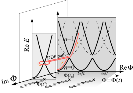
Figure 1: (color online) Many-body energy levels against the complex AB flux $\Phi$ for a finite, half-filled 1D Hubbard model ($L=10,\;N_{\uparrow}=N_{\downarrow}=5$, $U=0.5$). Only charge excitations are plotted. Quantum tunneling occurs between the groundstate (labeled as $n=0$) and a low-lying excited state ($n=1$) as the flux $\Phi(t)=Ft$ increases on the real axis, while the tunneling is absent for the states plotted as dashed lines. The wavy lines starting from the singular points ($\times$) at $\Phi(t^{*})$ represent the branch cuts for different Riemann surfaces, along which the solutions $n=0$ and $n=1$ are connected. In the DDP approach, the tunneling factor is calculated from the dynamical phase associated with adiabatic time evolution (DDP path) that encircles a gap-closing point at $\Phi(t^{*})$ on the complex $\Phi$ plane.

Here we consider the time evolution of electrons in a strong electric field $E$ for the one-dimensional Hubbard model,

$$H=-\sum_{i,\sigma}\left(e^{i\Phi(t)}c_{i+1\sigma}^{\dagger}c_{i\sigma}+\mbox{h.c.}\right)+U\sum_{i}n_{i\uparrow}n_{i\downarrow},$$ (1)

where the electric field is introduced by a time-dependent phase $\Phi(t)=Ft$ with $F=eE$ switched on at $t=0$. This is one obvious way of introducing an electric field through Faraday’s law. We have taken the absolute value of the hopping as the unit of energy. We study a half-filled, nonmagnetic case with numbers of electrons $N_{\uparrow}=N_{\downarrow}=L/2$ with $L$ the total number of sites. The Mott-insulator groundstate becomes unstable when the electric field becomes strong enough, for which charge excitations take place due to nonadiabatic quantum tunneling Oka2003 . In order to describe the process we introduce the adiabatic levels $|\psi_{n}(\Phi)\rangle$ that satisfy $H(\Phi)|\psi_{n}(\Phi)\rangle=E_{n}(\Phi)|\psi_{n}(\Phi)\rangle$ with $n=0,1,\ldots$, where $n=0$ corresponds to the groundstate. We neglect spin excitations to concentrate on charge excitations. The time evolution for $t>0$ is described by the time dependent Schrödinger equation, $i\frac{d}{dt}|\psi(t)\rangle=H(t)|\psi(t)\rangle$, with initial state $|\psi(t=0)\rangle=|\psi_{0}(\Phi=0)\rangle$. Figure 1 plots the adiabatic energy levels obtained by exact diagonalization for a small system. Nonadiabatic quantum tunneling between the groundstate and the lowest charge-excited state is most relevant (while the transition to the state represented by dashed lines is absent due to symmetry reasons). The adiabatic levels are periodic in $\Phi$ with a period $2\pi/L$, so that the tunneling from the groundstate to the excited state repeatedly occurs with a time interval $T=2\pi/FL$. We define the tunneling factor between the two states by $\gamma_{0\to 1}$ which is related to the transition probability $P=e^{-\gamma_{0\to 1}}$ for a single tunneling event. The solution of the time-dependent Schrödinger equation behaves as $|\psi(mT)\rangle\sim(1-e^{-\gamma_{0\to 1}})^{m/2}e^{i\alpha(t)}|\psi_{0}(t)\rangle$ with a phase factor $\alpha$, and the groundstate decay rate $\Gamma$ defined by $|\langle\psi_{0}(\Phi(t))|\psi(t)\rangle|^{2}=e^{-\Gamma t}$ becomesOka2005a $\Gamma/L\sim-\frac{F}{2\pi}\ln(1-e^{-\gamma_{0\to 1}})$. A naive estimate for the tunneling factor can be made by approximating the Hamiltonian in the vicinity of the transition by a Landau-Zener form, $H^{\rm LZ}=(^{vt\;\Delta/2}_{\Delta/2\;-vt})$, which leads to a threshold behavior with threshold $F_{\rm th}^{\rm LZ}$ given by Oka2003 ; Oka2005a

$$\gamma^{{\rm LZ}}_{0\to 1}=\pi\frac{F_{\rm th}^{\rm LZ}}{F},\;\;\;F_{\rm th}^{\rm LZ}=\frac{(\Delta/2)^{2}}{v},$$ (2)

where $\Delta$ is the charge gap (Mott gap) Lieb:1968AM , and $v$ is the slope of the adiabatic levels ($v\sim 2$ when $U$ is small and the system size is small). However, this expression should fail when the system size exceeds the localization lengthStafford1993 , since the slope vanish $v\to 0$ and the levels become flat against $\Phi$. Then, the transition probability also vanishes. But this obviously contradicts with a physical intuition that dielectric breakdown should take place in infinite systems. The point is that quantum tunneling can take place even when the levels are flat RozenZener .

In order to resolve this problem we introduce the DDP method which accommodates the thermodynamic limit as we shall see. In the general formalism of DDP the solution of the Schrödinger equation is extended to complex time; The tunneling process is described by an adiabatic evolution of the wave function along a path in the complex plane (DDP path in Fig. 1, displayed for a finite system for clarity). The DDP path encircles the point $t^{*}$ (exceptional point) on the complex $t$ plane at which the two energy levels cross, i.e., $E_{1}(\Phi(t^{*}))=E_{0}(\Phi(t^{*}))$. There is a branch cut starting from $t^{*}$ at which the two Riemann surfaces corresponding to $E_{0}$ and $E_{1}$ merge, and along a path encircling $t^{*}$ the solution $|\psi_{0}\rangle$ is deformed into the excited state $\propto|\psi_{1}\rangle$ with a proportionality factor determined by the complex dynamical phase. This gives a DDP tunneling probability $P=e^{-\gamma^{{\rm DDP}}_{0\to 1}}$ with Dykhne1962 ; DavisPechukas1976 ; PhysRevA.59.4580 ; Wilkinson2000

$$\gamma^{{\rm DDP}}_{0\to 1}=2\mbox{Im}S_{0,1}/\hbar,$$ (3)

where $S$ is the dynamical phase given by

$$S_{0,1}=\int_{t_{0}}^{t^{*}}dt^{\prime}[E_{1}(\Phi(t^{\prime}))-E_{0}(\Phi(t^{\prime}))],$$ (4)

with $t_{0}$ the starting point on the real axis.

We want to apply the DDP method (eqns. (3), (4)) to the Hubbard model, which means that we have to analytically continue the solutions to complex $\Phi$ for the first excited state ($E_{1}$) as well as for the groundstate ($E_{0}$). The Hubbard model with the phase factor (eqn. (1)) is exactly solvable with the Bethe ansatz method (see for example kusakabe ). This remains the case, for the groundstate, even when $\Phi$ is complex as demonstrated by Fukui and Kawakami Fukui . However, we have to extend the procedure to the excited states (Fig. 2), which is feasible with Woynarovich’s method Woynarovich1982 , where our goal is to calculate the energy difference $E_{1}(\Phi)-E_{0}(\Phi)$ for complex $\Phi$ and perform the integral along the DDP path. The DDP path (Fig.1) for the Hubbard model starts from $\Phi_{0}=\pi/L$ and ends at $\Phi_{*}=\pi/L+i\Psi_{\rm cr}$, where $\Psi_{\rm cr}$ is the value at which the gap closes Fukui . In the large $L$ limit the path lies on the imaginary axis.

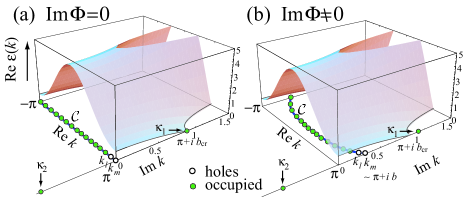
Figure 2: (color online) Schematic configurations (displayed here for $U=4.0$) of the charge rapidities for the lowest charge-excited state $|\psi_{1}(i\Psi)\rangle$ for $\Psi=0$(a), and for a finite $\Psi$(b). $\mathcal{C}$ corresponds to the groundstate continuum with occupied states (green circles, printed grey). In the excited state, two holes $k_{l},\;k_{m}$ (open circles) near $\pi+ib$ appear in the continuum, while two rapidities $\kappa_{1},\;\kappa_{2}$ outside the continuum $\mathcal{C}$ are occupied. The surface represents the real part of the excitation energy $\mbox{Re}\,\varepsilon(k)$ (plotted here for $\mbox{Re}\,\varepsilon(k)\geq 0$, $\mbox{Im}\,k>0$) which gives the energies of holes at $k_{l},k_{m}$. At $\Psi=0$, $\kappa_{1},\kappa_{2}$ sit on the $\mbox{Re}\,\varepsilon(k)=0$ curve.

We start with the Lieb-Wu Bethe-ansatz equation for an $L$-site Hubbard model with an imaginary $\Phi=i\Psi$,

$$Lk_{j}=2\pi I_{j}+iL\Psi-\sum_{\alpha=1}^{N_{\downarrow}}\theta(\sin k_{j}-\lambda_{\alpha}),$$ (5)

$$\sum_{j=1}^{L}\theta(\sin k_{j}-\lambda_{\alpha})=2\pi J_{\alpha}-\sum_{\beta=1}^{N_{\downarrow}}\theta\left(\frac{\lambda_{\alpha}-\lambda_{\beta}}{2}\right),$$ (6)

where $k_{j}\;(\lambda_{\alpha})$ are the charge (spin) rapidities, $\theta(x)=-2\mbox{arctan}(x/u)$ with $u=U/(4t)$ is the two-body phase shift, and $I_{j}\equiv N_{\downarrow}/2\;(\mbox{mod}~{}1),\;J_{\alpha}\equiv(N-N_{\downarrow}+1)/2\;(\mbox{mod}~{}1)$.

In the infinite-size limit, the Lieb-Wu equation for a finite $\Psi$ can be solved with the analytically continued charge and spin distribution functions Fukui . If we introduce the counting functions $z_{c}(k_{j})=I_{j}/L$ and $z_{s}(\lambda_{\alpha})=J_{\alpha}/L$, the Lieb-Wu equation in the bulk limit reads

$$z_{c}(k) = \frac{k}{2\pi}-\frac{i\Psi}{2\pi}-\frac{1}{2\pi}\int_{\mathcal{S}}d\lambda\,\theta(\sin k-\lambda)\sigma^{*}(\lambda),$$ (7)

$$z_{s}(\lambda) = \frac{1}{2\pi}\int_{\mathcal{C}}dk\,\theta(\sin k-\lambda)\rho^{*}(k)$$ (8)

$$+\frac{1}{2\pi}\int_{\mathcal{S}}d\lambda^{\prime}\,\theta\left(\frac{\lambda-\lambda^{\prime}}{2}\right)\sigma(\lambda^{\prime}),$$

where the distribution functions are defined by $\rho(k)=\partial_{k}z_{c}(k),\;\sigma(\lambda)=\partial_{\lambda}z_{s}(\lambda)$, and $\sigma^{*},\sigma,\rho^{*}$ are explained around eqn. (11) below. The contours $\mathcal{C}$ and $\mathcal{S}$, i.e., the continuum limit of the charge ($\mathcal{C}$) and spin ($\mathcal{S}$) rapidities’ positions, are of great importance. In fact, for the groundstate, the paths are determined such that the conventional solutionLieb:1968AM , $\rho_{0}(k)=\frac{1}{2\pi}+\frac{1}{2\pi}\cos k\int_{0}^{\infty}\frac{e^{-u\omega}}{\cosh u\omega}J_{0}(\omega)\cos(\omega\sin k)d\omega$ and $\sigma_{0}(\lambda)=\frac{1}{2\pi}\int_{0}^{\infty}\frac{J_{0}(\omega)\cos\omega\lambda}{\cosh u\omega}d\omega$ with $J_{n}$ Bessel’s function, extended to complex $k$ and $\lambda$ solves eqns. (7), (8). This determines the end point of contour $\mathcal{C}$, which we denote $\pm\pi+ib$ (Fig. 2), where $b$ is an increasing function of $\Psi$ satisfying Fukui

$$\Psi=b-i\int_{-\infty}^{\infty}d\lambda\theta(\lambda+i\sinh b)\sigma_{0}(\lambda).$$ (9)

We denote the end point corresponding to $\Psi=\Psi_{\rm cr}$ to be $b=b_{\rm cr}$. The end point of $\mathcal{S}$ is $\lambda=\pm\pi$.

Woynarovich’s construction Woynarovich1982 of charge excitations can be applied to the non-Hermitian case ($\Psi\neq 0$) with the same contours $\mathcal{C}$, $\mathcal{S}$ as in the groundstate. The idea is to remove two charge rapidities $k_{l},\;k_{m}$ from $\mathcal{C}$ and one spin rapidity $\lambda_{N_{\downarrow}/2}$ from $\mathcal{S}$ to place them on the complex $k$ and $\lambda$ planes at positions $\kappa_{1},\;\kappa_{2}$ and $\Lambda$, respectively (Fig. 2) in such a way that the Lieb-Wu equation is satisfied, which yields

$$\sin(\kappa_{1,2})=\Lambda\pm iu,\quad\Lambda=(\sin k_{l}+\sin k_{m})/2.$$ (10)

With these parameters, the Lieb-Wu equation (8) for charge excitations can be solved by

$$\sigma(\lambda) = \sigma_{0}(\lambda)-\frac{1}{LU}\left\{\frac{1}{\cosh[(\lambda-\sin k_{l})\pi/2u]}\right.$$ (11)

$$+ \left.\frac{1}{\cosh[(\lambda-\sin k_{m})\pi/2U]}\right\},$$

$$\rho(k) = \rho_{0}(k)+\frac{1}{2\pi L}\cos k\frac{u}{u^{2}+(\sin k-\Lambda)^{2}}$$ (12)

$$-\frac{\cos k}{2\pi L}\int_{0}^{\infty}\frac{e^{-\omega u}}{\cosh\omega u}\{\cos[\omega(\sin k-\sin k_{l})]$$

$$+\cos[\omega(\sin k-\sin k_{m})]\}d\omega,$$

with which we can define $\sigma^{*}(\lambda)=\sigma(\lambda)+(1/L)\delta(\lambda-\Lambda),\;\rho^{*}(k)=\rho(k)-(1/L)\delta(k-k_{l})-(1/L)\delta(k-k_{m})$ appearing above. We note that these equations are identical with Woynarovich’s, which is natural since the operations $\partial_{k},\partial_{\lambda}$ do not pick up $\Psi$, while $\Psi$ controls the integration path via eq.(9). The energy of the excited state can be calculated from $\rho^{*}(k)$, which gives $E_{1}(\Psi)-E_{0}(\Psi)=\varepsilon(k_{l})+\varepsilon(k_{m})$ with $E_{0}$ the groundstate energy, and the $\varepsilon(k)$ given as

$$\varepsilon(k) = 2u+2\cos(k)$$

$$+2\int_{0}^{\infty}\frac{e^{-u\omega}}{\omega\cosh u\omega}J_{1}(\omega)\cos(\omega\sin k)d\omega.$$

The lowest excited state is given by setting $k_{l},k_{m}\simeq\pi+ib$ in the above solution (Fig.2). We can specify the deformation of the Bethe ansatz solution along the DDP path (Fig. 1) as follows. As $\Psi$ becomes finite, the end points of $\mathcal{C}$, i.e., $\pm\pi+ib$, move along the imaginary axis until $b$ reaches $b_{\rm cr}$ at which the gap closes, i.e., $E_{1}-E_{0}=0$ (Fig. 3, inset)Fukui . Meanwhile, $\mbox{Im}\,\kappa_{1}$ and $\mbox{Im}\,\kappa_{2}$ increase with $\Psi$, where $\kappa_{2}$ in particular touches the real axis at the critical point. From the DDP formula (eqns. (3), (4)), the quantum tunneling probability $P=e^{-\pi F_{\rm th}^{\rm DDP}/F}$ has the threshold electric field,

$$F_{\rm th}^{\rm DDP}=\frac{2}{\pi}\int_{0}^{b_{\rm cr}}(E_{1}-E_{0})\frac{d\Psi}{db}db$$ (14)

$$= \frac{2}{\pi}\int_{0}^{\sinh^{-1}u}4\left[u-\cosh b+\int_{-\infty}^{\infty}d\omega\frac{e^{\omega\sinh b}J_{1}(\omega)}{\omega(1+e^{2u|\omega|})}\right]$$

$$\times\left[1-\cosh b\int_{0}^{\infty}d\omega\frac{J_{0}(\omega)\cosh(\omega\sinh b)}{1+e^{2u\omega}}\right]db.$$

Its $U$-dependence is plotted e in Fig. 3 (a) (solid line), which confirms the collective nature of the breakdown (i.e., the threshold much smaller than a naive $U$). In other words, the tunneling takes place not between neighboring sites, but over an extended region due to a leakage of the many-body wave function, where the size is roughly the localization length Stafford1993 .

Let us now compare the present analytical result with the numerical one in Fig. 3 (a), which plots $F_{\rm th}^{\rm DDP}$ along with the threshold obtained by the time-dependent density-matrix renormalization group (DMRG) for an $L=50$, open Hubbard chain Oka2005a . The agreement between the analytical and numerical results is excellent.

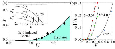
Figure 3: (a) The threshold field strength $F$ against $U$ obtained by the present DDP formalism (solid line; eqn. (14)). Inset: The energy difference between the groundstate and the excited state against $b$ for various values of $U$. (b) The decay rate $\Gamma$ of the groundstate against the electric field $F$ obtained by the DDP formalism (solid line; eqn.(15)). In (a) and (b), the symbols represent the time-dependent DMRG result Oka2005a .

Finally, let us say a few words about the dynamics that takes place after the electric field exceeds the threshold. There are infinitely many excited states whose energies are larger but near $|\psi_{1}\rangle$’s, and tunneling becomes also activated to these states. The net tunneling to such states is incorporated in the groundstate decay rate $\Gamma/L$ (defined above eqn.(2)). This quantity has been numerically calculated with the time-dependent DMRG in ref.Oka2005a , where the single-tunneling formula reduced by an empirical factor $a<1$,

$$\Gamma/L=-\frac{aF}{2\pi}\ln[1-\exp(-\pi F_{\rm th}^{\rm DDP}/F)],$$ (15)

is found to describe the numerical result. The present DDP result again exhibits an excellent agreement with the numerical one (Fig. 3(b)). This implies that the tunneling to higher excited states do not change the threshold, while the decay rate is reduced due to the pair-annihilation processesOka2005a . We note that the decay rate is an experimental observable which can be obtained from the delay time of the current (the production rate in ref. tag Fig. 4), and the present theory is consistent with the experimental result. The nature of the nonequilibrium steady state above the threshold is an interesting problem, which will be addressed elsewhere where an electron avalanche effect is evoked for the metallization.

In conclusion, we have shown that the DDP theory of quantum tunneling combined with a generalized Bethe ansatz describes the nonlinear transport and dielectric breakdown of the 1D Mott insulator. This is the first analytical result obtained on nonequilibrium properties in correlated electron system, and the DDP method is expected to have potential applicability to many other models and problems. We wish to thank Mitsuhiro Arikawa, Yasuhiro Hatsugai and Takahiro Fukui for fruitful discussions, and Seiji Miyashita for bringing our attention to RozenZener . HA was supported by a Grant-in-Aid for Scientific Research on Priority Area “Anomalous quantum materials”, TO by a Grant-in-Aid for Young Scientists (B) from MEXT.

References

- (1) M. Imada, A. Fujimori, and Y. Tokura, Rev. Mod. Phys. 70, 1039, (1998).
- (2) Y. Taguchi, T. Matsumoto, and Y. Tokura, Phys. Rev. B 62, 7015 (2000).
- (3) T. Fukui and N. Kawakami, Phys. Rev. B 58, 16051 (1998).
- (4) T. Oka, R. Arita, and H. Aoki, Phys. Rev. Lett. 91, 66406 (2003).
- (5) T. Oka, and H. Aoki, Phys. Rev. Lett. 95, 137601 (2005).
- (6) M. Greiner et al, Nature 415, 39 (2002).
- (7) M. Jona-Lasinio et al.,Phys. Rev. Lett.91, 230406 (2003).
- (8) L. Fallani et al., Phys. Rev. Lett. 93,140406 (2004).
- (9) D. Witthaut et al., Phys. Rev. A 73, 063609 (2006).
- (10) U. Schneider et al., Science 322, 1520 (2008).
- (11) J. Schwinger, Phys. Rev. 82, 664 (1951).
- (12) A. G. Green and S. L. Sondhi, Phys. Rev. Lett. 95, 267001 (2005).
- (13) A. M. Dykhne, Sov. Phys. JETP 14, 941 (1962).
- (14) J. P. Davis and P. Pechukas, J. Chem. Phys. 64, 3129 (1976).
- (15) N. Hatano and D. R. Nelson, Phys. Rev. Lett. 77, 570 (1996).
- (16) Y. Nakamura and N. Hatano, J. Phys. Soc. Jpn. 75, 104001 (2006).
- (17) E. H. Lieb and F. Y Wu, Phys. Rev. Lett 21, 192 (1968).
- (18) F. H. L. Essler, H. Frahm, F. Göhmann, A. Klümper, and V. E. Korepin, The One-Dimensional Hubbard Model, (Cambridge Univ. Press, 2005).
- (19) C. F. Coll, Phys. Rev. B 9, 2150 (1974).
- (20) A. A. Ovchinnikov, Sov. Phys. JETP 30, 1160 (1970).
- (21) M. Takahashi, Prog. Theor. Phys.47, 69 (1972).
- (22) F. Woynarovich, J. Phys. C 15, 85 (1982).
- (23) A famous example is the Rozen-Zener transition, N. Rozen and C. Zener, Phys. Rev. 40, 502 (1932).
- (24) N. V. Vitanov and K.-A. Suominen, Phys. Rev. A 59, 4580 (1999).
- (25) M. Wilkinson and M. A. Morgan, Phys. Rev. A 61, 062104 (2000).
- (26) K. Kusakabe and H. Aoki, J. Phys. Soc. Jpn 65, 2772 (1996).
- (27) C. A. Stafford and A. J. Millis, Phys. Rev. B 48, 1409 (1993).