Width of reaction zones in $A+B\rightarrow C$ type reaction-diffusion processes:
Effects of an electric current

Abstract

We investigate the effects of an electric current on the width of a stationary reaction zone in an irreversible $A^{-}+B^{+}\to C$ reaction-diffusion process. The ion dynamics of the electrolytes $A\equiv(A^{+},A^{-})$ and $B\equiv(B^{+},B^{-})$ is described by reaction-diffusion equations obeying local electroneutrality, and the stationary state is obtained by employing reservoirs of fixed electrolyte concentrations at the opposite ends of a finite domain. We find that the width of the reaction zone decreases when the current drives the reacting ions towards the reaction zone while it increases in the opposite case. The linear response of the width to the current is estimated by developing a phenomenological theory based on conservation laws and on electroneutrality. The theory is found to reproduce numerical solutions to a good accuracy.

I Introduction

The reaction-diffusion process $A+B\rightarrow C$ combined with the ensuing evolution of the reaction product $C$ (e.g. precipitation) underlie the explanation of a large number of physical, chemical, and biological phenomena Henisch ; kotomin ; Dani ; mathbiol . An interesting aspect of the reaction-diffusion part of these processes is the presence of reaction zones. They are formed either because the reagents $A$ and $B$ are initially separated zol or because spatial inhomogeneities exist in the initial distribution of the reagents Redner1 . These zones are important since by determining where and when the reaction product emerges, they set the stage for the temporal and spatial evolution of $C$s. Accordingly, the motion of these fronts, the spatial distribution of the rate of the production of $C$, and the width of the reaction zones have been much investigated. They are known theoretically for the case of neutral reagents zol ; Redner1 ; chopard ; cornell ; inhom ; redner and the theories have been verified in experiments Kopelman-1 ; Bazant ; Kopelman-3 ; Tabeling ; Kopelman-4 .

In realistic situations, however, the reagents $A$ and $B$ are often electrolytes which dissociate,

$$A\rightarrow A^{+}+A^{-}\,,\qquad B\rightarrow B^{+}+B^{-}\,,$$ (1)

and the reaction takes place between the ‘active’ ions which, for definiteness, will be taken below to be $A^{-}$ and $B^{+}$:

$$A^{-}+B^{+}\rightarrow C\,.$$ (2)

Although the counterions $A^{+}$ and $B^{-}$ are not reacting, they influence the dynamics significantly through the electroneutrality constraint so that the task of characterizing the front becomes much more involved rubinstein90 .

Some of the front properties such as the spatial location and the reaction product distribution (but not the width of the reaction zone) have nevertheless been obtained for ionic reactions in one-dimensional geometry unger . Furthermore, these studies have been extended to ions being driven by an electric current or by an external potential difference bena . The driven systems are of special interest when the $C$s undergo phase separation, since then they may be used to design bulk precipitation patterns. Indeed, it has been shown recently ourprl ; encoding that a flexible control of precipitation patterns can be achieved through controlling the reaction zones by appropriately designed time-dependent currents.

From the technological point of view, controlling precipitation patterns becomes relevant if the patterns can be downsized to the submicron range. Since the width of the reaction zones is one of the limiting factors in downsizing, it is clear that one should understand how to control it. The studies of the width for neutral reagents zol ; chopard ; cornell ; redner suggest that the parameter strongly affecting the width is the reaction rate constant. It is, however, not a parameter we can adjust, thus other means of control should be found. Since electric currents turned out to be useful in manipulating patterns ourprl ; encoding , it is natural to ask if the width could also be controlled by them. This is the question we address in this work.

In order to simplify the task, we restrict our study to a one-dimensional reaction-diffusion process on a finite interval. The concentrations of the electrolytes are fixed at the boundaries and, furthermore, a current generator is attached so that a constant current flows through the system (see Fig.1 and Fig.2). For this setup, we derive the reaction-diffusion equations in the long-time limit when the stationary state is reached. Solving these equations numerically (and, in some limits, analytically as well), we obtain the width of the stationary reaction front, $w(J)$, as a function of the electric current, $J$.

The $J=0$ case has been investigated earlier redner and we recover the zero current width, $w(0)$, obtained in that work. For $J\not=0$, our general finding is that a forward current (a current that drives the reacting ions towards the reaction zone) reduces the width of the stationary reaction zone, while a current of opposite polarity (backward current) increases the width. For small currents the change compared to the zero-current case is proportional to the current [$w(J)-w(0)\propto J$] with a proportionality constant that can be estimated from rather general reasoning and the results are found to compare favorably with the numerical solutions. Although our results concern the width of stationary states, we present some arguments that the quasistationary nature of the diffusive fronts allows the derivation of the dynamics of the width in some time window in case of moving fronts as well.

The paper is organized as follows. In Sec. II, we introduce the problem and discuss the equations describing the dynamics of the ions. Sec. III contains the derivation of the model equations for the particular case of the stationary state. Analytical and approximate solutions are obtained both for symmetric setup (Sec. IV) and asymmetric setup (Sec. V). Possible applications of the stationary state results to moving reaction front are presented in Sec. VI, and conclusions are drawn in Sec. VII.

II The Problem and the model

Fig.1 displays the setup for producing a stationary reaction zone in the presence of an electric current. Two dissociating electrolytes $A$ and $B$ [see Eq.(1)] are dissolved in a column of gel where their transport is restricted to be diffusive. The opposite ends of the columns are connected to reservoirs of $A$ and $B$, respectively, thus we fix the electrolyte concentrations $a_{0}$ and $b_{0}$ at the boundaries. Furthermore, we maintain a constant electric current through the system by attaching a current generator to the ends of the column separated by a distance $L$ (in another possible setup one keeps a fixed potential difference between the ends).

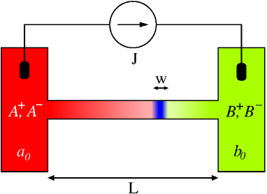
Figure 1: (Color online) Experimental setup for generating a stationary reaction front in the presence of an electric current. The details are described in the text.

As the reaction-diffusion dynamics proceeds, a reaction zone (a spatial region where the reaction $A^{-}+B^{+}\to C$ takes place i.e. where the rate of the production $R(x,t)$ of $C$s is nonzero, see Fig.2.) is formed. In the long-time limit the system relaxes to a stationary state and the front becomes stationary as well, $R(x,t)\to R(x)$. We shall be interested in the stationary state properties of the front, and particularly in its width $w$ which we can define e.g. through the second moment of the production rate

$$w^{2}=\frac{\int\,dx\,(x-x_{f})^{2}\,R(x)}{\int\,dx\,R(x)}$$ (3)

where the integrals are over the interval $[-L/2,L/2]$ and $x_{f}$ is the center of the reaction zone

$$x_{f}=\frac{\int\,dx\,x\,R(x)}{\int\,dx\,R(x)}\,.$$ (4)

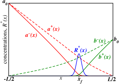
Figure 2: (Color online) Characteristic stationary profiles of the ion concentrations in the presence of an electric current. The rate of production $R(x)$ of $C$s is measured in units of $ka_{0}$ where $k$ is the rate constant of the reaction, and a magnification factor $10^{3}$ is used for better visibility, i.e. $R^{*}=10^{3}R(x)/ka_{0}$. The position of the front is denoted by $x_{f}$.

In order to calculate $w$, we shall use reaction-diffusion equations which amounts to a mean-field description of the problem. In addition, the following simplifying assumptions will be made:

(i) The system is treated as one-dimensional, i.e. all the relevant quantities are assumed to depend on a single spatial coordinate $x$, with $-L/2\leq x\leq L/2$ being the spatial extent of the system.

(ii) We consider instantaneous 100% dissociation of the electrolytes $A$ and $B$ according to Eq. (1) (this is the assumption of “ideally strong” acid and basis). Accordingly, only $A^{\pm}$ and $B^{\pm}$ ions (and the reaction product $C$) are present in the system.

(iii) The dynamics of the inert reaction product $C$ is assumed to have no feedback on the dynamics of the reagents.

(iv) The equations are assumed to satisfy electroneutrality rubinstein90 meaning that the local charge density is zero on relevant space scales ( in particular on the scale of the width of the reaction zone), i.e.

$$\sum_{i}z_{i}\,n_{i}(x,t)=0\,,$$ (5)

where $z_{i}$ is the charge of the $i$-th ion – in terms of the elementary charge $q$ – and $n_{i}(x,t)$ denotes its density.

(v) Monovalent ions, i.e. $|z_{i}|=1$ for all $i$ will be considered.

(vi) We assume equal diffusion coefficients for the ions, i.e. $D_{i}=D$ for all $i$.

(vii) The boundary conditions follow from the assumption that there are infinite reservoirs providing fixed concentrations of the ions at the border . Denoting the concentration profiles of the $A^{\pm}$ and $B^{\pm}$ ions by $a^{\pm}(x,t)$ and $b^{\pm}(x,t)$, respectively, the boundary conditions then can be written as

$$a^{+}(-L/2,t)=a^{-}(-L/2,t)={a_{0}}\,$$ (6)

$$b^{+}(-L/2,t)=b^{-}(-L/2,t)=0\,$$ (7)

$$a^{+}(L/2,t)=a^{-}(L/2,t)=0,\,$$ (8)

$$b^{+}(L/2,t)=b^{-}(L/2,t)=b_{0}\,.$$ (9)

Since we are interested in the stationary state, the detailed initial conditions are irrelevant provided the reagents are separated initially. Some dynamical properties, but not the width, have already been investigated for a similar setup bena for the case $a_{0}\ll b_{0}$ where the initial conditions lead to a moving front.

The general evolution equations for the concentration profiles $a^{\pm}(x,t)$ and $b^{\pm}(x,t)$ were derived in bena . For the simplified case we are considering here, they acquire the following form:

$$\frac{\partial a^{-}(x,t)}{\partial t} = D\frac{\partial^{2}a^{-}}{\partial x^{2}}+\lambda\frac{\partial(a^{-}{E})}{\partial x}-ka^{-}b^{+}$$ (10)

$$\frac{\partial b^{+}(x,t)}{\partial t} = D\frac{\partial^{2}b^{+}}{\partial x^{2}}-\lambda\frac{\partial(b^{+}{E})}{\partial x}-ka^{-}b^{+}$$ (11)

$$\frac{\partial a^{+}(x,t)}{\partial t} = D\frac{\partial^{2}a^{+}}{\partial x^{2}}-\lambda\frac{\partial(a^{+}{E})}{\partial x}$$ (12)

$$\frac{\partial b^{-}(x,t)}{\partial t} = D\frac{\partial^{2}b^{-}}{\partial x^{2}}+\lambda\frac{\partial(b^{-}{E})}{\partial x}\,.$$ (13)

Here $D$ are the diffusion coefficients of the ions, $k$ is the rate constant of the reaction $A^{-}+B^{+}\to C$, $\lambda=DF/RT$ with $F=qN_{A}$ being the Faraday’s constant (i.e., the electric charge transported by a mole of monovalent positive ions), $R$ is the universal gas constant, and $T$ is the temperature.

The scaled local electric field $\lambda E(x,t)$ in the above equations is obtained from the local electroneutrality assumption, and it is given by rubinstein90 ; bena :

$$\lambda E(x,t)=\frac{J(t)}{q\,\left(\,a^{+}+a^{-}+b^{+}+b^{-}\,\right)}.$$ (14)

where $J(t)$ is the electric current density, flowing through the system. In view of the electroneutrality condition, $J(t)$ is divergence-free, i.e., for the one-dimensional case it can depend only on time.

At this point, there are two ways to proceed. If a current generator is used and the current is fixed to be constant, $J(t)\equiv J$, then Eq.(14) determines $E(x,t)$ and thus Eqs.(10-14) together with the boundary conditions Eqs.(6-9) form the closed set of equation to be solved. This is the case we shall treat in detail below.

Experimentally, it may be more convenient to maintain a constant voltage difference $U=V(L)-V(0)$ instead of a constant current. In that case, integrating Eq.(14) yields

$$\int\limits_{-L/2}^{L/2}dx{E(x,t)}=\int\limits_{-L/2}^{L/2}dx\frac{J(t)}{\lambda q\left(\,a^{+}+a^{-}+b^{+}+b^{-}\,\right)}=-U$$ (15)

and so $J(t)$ is given through $U$. Then, substituting $J(t)$ into Eq.(14), one finds the scaled field $\lambda E$

$$\lambda E(x,t)=-\lambda U\,\frac{\left(\,a^{+}+a^{-}+b^{+}+b^{-}\,\right)^{-1}}{\int\limits_{-L/2}^{L/2}dx\,\left(\,a^{+}+a^{-}+b^{+}+b^{-}\,\right)^{-1}}$$ (16)

thus arriving at a closed set of Eqs.(10-13).

It should be noted that the constant $U$ and constant $J$ cases are equivalent provided only the stationary states are considered. Indeed, the concentrations are time independent in the stationary state and, consequently, it follows from Eq.(15) that constant $U$ implies that $J$ is independent of time, thus we returned to the constant current case. One cannot give, however, a simple relation between $U$ and $J$ since, as can be seen from Eq.(15), the proportionality constant depends on the stationary state reached for a given $U$ or $J$.

III Stationary state

The equations for the stationary solution $n_{i}(x,t)\equiv n_{i}(x)$ are obtained by setting the time derivatives to zero in Eqs.(10-13). To make the equations more transparent one can introduce dimensionless quantities by measuring $x$ in units of $L$ and the concentrations $n_{i}$ in units of $a_{0}$. Then, substituting Eq.(14) with $J(t)=J$ into Eqs.(10-13) (i.e. considering the constant current case), we obtain

$$(a^{-})^{{}^{\prime\prime}}+J_{0}\left(\frac{a^{-}}{a^{+}+a^{-}+b^{+}+b^{-}}\right)^{{}^{\prime}}-k_{0}a^{-}b^{+}=0\quad$$ (17)

$$(b^{+})^{{}^{\prime\prime}}-J_{0}\left(\frac{b^{+}}{a^{+}+a^{-}+b^{+}+b^{-}}\right)^{{}^{\prime}}-k_{0}a^{-}b^{+}=0\quad$$ (18)

$$(a^{+})^{{}^{\prime\prime}}-J_{0}\left(\frac{a^{+}}{a^{+}+a^{-}+b^{+}+b^{-}}\right)^{{}^{\prime}}=0\quad$$ (19)

$$(b^{-})^{{}^{\prime\prime}}+J_{0}\left(\frac{b^{-}}{a^{+}+a^{-}+b^{+}+b^{-}}\right)^{{}^{\prime}}=0\quad$$ (20)

where prime denotes the spatial derivatives, and

$$J_{0}=\frac{JL}{qDa_{0}}\quad,\quad k_{0}=\frac{ka_{0}L^{2}}{D}\,.$$ (21)

In order to solve the above equations the rescaled current $J_{0}$ and rate constant $k_{0}$, and the boundary condition $b_{0}/a_{0}$ should be given. In principle, we could proceed then by numerically solving the equations.

We would like, however, to find first some analytical estimates of $w(J_{0})$. For this purpose, we begin by considering a symmetric setup where $a_{0}=b_{0}$ and the $k_{0}\to\infty$ limit is taken. In this case, $J_{0}$ remains the only control parameter, and the reaction zone becomes pointlike. The limit is nevertheless relevant. First, because the real reaction zones are narrow, in general. Second, because the analytical estimates of the sensitivity of concentration profiles to small currents can be used to estimate the width for $k_{0}$ finite but large. Once the phenomenological estimate of $w(J_{0})$ is obtained, we carry out numerical investigations as well to judge the accuracy of the phenomenology. In a final step, the results will be generalized to the $a_{0}\not=b_{0}$ case.

IV Symmetric setup ($a_{0}=b_{0}$)

IV.1 Point reaction zone (infinite reaction rate)

The reaction zone is pointlike for $k_{0}\to\infty$, and it follows from the symmetry of the $a_{0}=b_{0}$ setup that the position of the reaction zone is at $x_{f}=0$. The concentrations of the reacting ions satisfy $a^{-}(x>0)=0$ and $b^{+}(x<0)=0$ and so we have two sets of equations for the two sides of the front. We begin by considering the left-hand side ($x<0$) and obtain the concentration on the right-hand side by symmetry, namely $b_{x>0}^{+}(x)=a_{x<0}^{-}(-x)$, $b_{x>0}^{-}(x)=a_{x<0}^{+}(-x)$ and $a_{x>0}^{+}(x)=b_{x<0}^{-}(-x)$.

The equation for $x<0$ are found by setting $b^{+}=0$ in Eqs.(17,19,20):

$$(a^{-})^{{}^{\prime\prime}}+J_{0}\left(\frac{a^{-}}{a^{+}+a^{-}+b^{-}}\right)^{\prime} = 0\quad$$ (22)

$$(a^{+})^{{}^{\prime\prime}}-J_{0}\left(\frac{a^{+}}{a^{+}+a^{-}+b^{-}}\right)^{\prime} = 0\quad$$ (23)

$$(b^{-})^{{}^{\prime\prime}}+J_{0}\left(\frac{b^{-}}{a^{+}+a^{-}+b^{-}}\right)^{\prime} = 0\quad.$$ (24)

The boundary conditions to the above equations at $-L/2$ [see Eqs.(6,7)] do not change while, at the reaction zone, the following boundary conditions must be used

$$a^{-}(0) = 0\,,$$ (25)

$$b^{-}(0) = a^{+}(0)\,,$$ (26)

$$\left.(a^{+})^{\prime}\right|_{x=0} = -\left.(b^{-})^{\prime}\right|_{x=0}\quad.$$ (27)

The first equality follows from the infinite rate constant. The second one is the electroneutrality condition ($a^{+}-a^{-}-b^{-}=0$) employed at the reaction zone. Finally, the third condition follows from the requirement that, for the counterions, not only their concentrations but also their derivatives should be continuous across the reaction zone.

The first step in solving the equations for $x<0$ is the application of the electroneutrality condition ($a^{+}-a^{-}-b^{-}=0$) to Eq.(23). It yields $(a^{+})^{{}^{\prime\prime}}=0$, thus resulting in the following solution for $a^{+}$:

$$a^{+}(x)=1+A\left(2x+1\right)$$ (28)

where we used the boundary condition at $x=-L/2$. The integration constant $A$ remains undetermined at this stage.

Having the solution for $a^{+}(x)$, and using the electroneutrality condition in Eq.(22), we find now that $a^{-}$ satisfies the following equation

$$(a^{-})^{\prime}+\frac{J_{0}}{2}\frac{a^{-}}{1+A(2x+1)}=I_{1}\\$$ (29)

where $I_{1}$ is another integration constant.

The general solution of equation (29) reads

$$a^{-}(x)=C_{1}[1+A(2x+1)]+C_{2}[1+A(2x+1)]^{\Delta}\,,$$ (30)

and the boundary conditions provide $C_{1}$ and $C_{2}$

$$C_{1} = -\frac{(1+A)^{\Delta-1}}{1-(1+A)^{\Delta-1}}$$ (31)

$$C_{2} = \frac{1}{1-(1+A)^{\Delta-1}}$$ (32)

with $\Delta=-J_{0}/4A$.

Once $a^{-}$ and $a^{+}$ are known, $b^{-}$ is obtained from the electroneutrality condition $b^{-}=a^{+}-a^{-}$. Thus what remained is to determine the integration constant $A$. We can find $A$ by combining the electroneutrality condition with the boundary condition Eq.(27) to arrive at

$$\left.(a^{-})^{\prime}\right|_{x=0}=2\left.(a^{+})^{\prime}\right|_{x=0}\,.$$ (33)

Substituting now Eqs. (28) and (30) into Eq.(33), we obtain $A$ as the solution of the following relation:

$$\left(1-\frac{J_{0}}{4A}\right)(1+A)^{-(1+\frac{J_{0}}{4A})}=2\;.$$ (34)

We have thus determined all the concentration profiles for $x<0$ and, as mentioned above, the profiles for $x>0$ can be obtained from symmetry considerations.

IV.2 Reaction rate and the slope of $a^{-}$ at $x=0$

A simple question one might ask about the $k_{0}\to\infty$ case is the following: How does the rate of reaction changes when the current is switched on? In order to calculate this quantity, the slope $(a^{-})^{\prime}$ needs to be evaluated at the reaction zone ($x=0$). As we shall see, the same slope will also be important in the next Subsection IV.3 where a phenomenological estimate of the width $w(J)$ will be carried out.

The derivative $\left.(a^{-})^{\prime}\right|_{x=0}$ can be calculated by noting from Eq.(33) that $\left.(a^{-})^{\prime}\right|_{x=0}=2\left.(a^{+})^{\prime}\right|_{x=0}$ and that $(a^{+})^{\prime}=2A$ follows from Eq.(28). As a result, we arrive at

$$\left.(a^{-})^{\prime}\right|_{x=0}=4A\,.$$ (35)

The rate of reaction is the flux of the reacting ions $j$ into the reaction zone. It is the number of $A^{-}$ ions reaching $x=0$ in unit time, and is obtained as

$$j(J_{0})=-\left.(a^{-})^{\prime}\right|_{x=0}-\left.\frac{J_{0}a^{-}}{a^{+}+a^{-}+b^{-}}\right|_{x=0}\quad.$$ (36)

where we note that $j$ is also scaled quantity, i.e. it is measured in units of $Da_{0}/L$. Since $\left.a^{-}\right|_{x=0}=0$, the second term on the right-hand side is zero. The first one is obtained from Eq.(35), thus yielding

$$j(J_{0})=-\left.(a^{-})^{\prime}\right|_{x=0}=-4A(J_{0})$$ (37)

where $A(J_{0})$ is given by solving Eq.(34).

Analytic expressions of $j(J_{0})$ can be developed for small $J_{0}$ since we can expand the solution of Eq.(34) in powers of $J_{0}\ll 1$. To first order in $J_{0}$, we find $A(J_{0})=-1/2+(1-\ln 2)J_{0}/4$ and consequently

$$j(J_{0})=-\left.(a^{-})^{\prime}\right|_{x=0}=2-(1-\ln 2)J_{0}\quad.$$ (38)

Introducing the scaled flux $\tilde{j}_{0}$ of $A^{-}$ ions in the absence of electric current ($\tilde{j}_{0}=2$), we can write the expansion as

$$j(J_{0})=\tilde{j_{0}}\left(1-\alpha\frac{J_{0}}{\tilde{j_{0}}}\right)\quad.$$ (39)

where $\alpha=1-\ln{2}>0$.

Let us consider now the sign of the first order contribution. Note that $J_{0}\sim J$ and it follows from Eqs.(10-13) that $J<0$ means that the negative (positive) ions are driven to the right (left). In this case, the reacting ions are driven towards the reaction zone and the first order correction is positive and, consequently, the reaction rate increases [$j(J_{0})>\tilde{j_{0}}$]. We shall call the $J<0$ electric current as forward current. The reagents are driven away from the reaction zone in the opposite case ($J>0$, backward current) and, as expected, the reaction rate decreases [$j(J_{0})<\tilde{j_{0}}$].

An important point to recognize here is that the change in the reaction rate does not come directly from the drift term in the flux of particles, it comes indirectly from the change in the diffusive flux i.e. from the change in the slope of the reaction profiles near the reaction zone. We shall see a similar effect when calculating the width of the reaction zone.

In closing this section, we display the diffusive flux $-D(a^{-})^{\prime}$ in terms of the original variables

$$\left.-D(a^{-})^{\prime}\right|_{x=0}=2\frac{a_{0}D}{L}+(1-\ln 2)\frac{J}{q}=j_{0}-\alpha\frac{J}{q}\quad.$$ (40)

where $j_{0}=2a_{0}D/L$ is the unscaled diffusive flux in the absence of electric current. We shall need the above expression in the phenomenological arguments of the next section which would be less transparent using the scaled variables.

IV.3 Finite reaction rate: Phenomenological considerations and numerical solutions

For the limiting case of an infinite rate constant ($k_{0}\to\infty$), we have analytical solutions for the concentration profiles for arbitrary $J_{0}$. The physically relevant case, however, is the one with finite $k_{0}$ where there is little hope to find exact solutions. For this case, we developed phenomenological considerations which have their roots in the success of similar arguments for simpler cases zol ; Redner1 , and we expect it to be performing well at least for small currents. As we shall see, the validity of the phenomenological argument is supported by numerical integration of the original equations.

The main idea is to use the balance equation for the reacting ions, namely to equate the number of reactions per unit time to the flux of reacting ions towards the reaction zone. To do this, one needs the values of the concentrations and their derivatives. They are estimated by assuming that the concentration profiles are smooth functions and, for finite but large $k_{0}$, their slopes in the reaction zone can be approximated by the $k_{0}\to\infty$ values.

The balance equation can be obtained by integrating eq.(17) through the reaction zone i.e. from $-w$ to $w$

$$\left.-D\frac{da^{-}}{dx}\right|_{-w}-\frac{J}{q}\left.\frac{a^{-}}{a^{+}+a^{-}+b^{+}+b^{-}}\right|_{-w}=k\overline{a^{-}}\cdot\overline{b^{+}}w\,.$$ (41)

Here the upper bars represent the spatial averages over the reaction zone and, in the spirit of mean-field approximation, the average of the product $\overline{a^{-}b^{+}}$ has been replaced by the product of averages $\overline{a^{-}}\cdot\overline{b^{+}}$. Furthermore, the contribution from the upper limit of the integrals on the left-hand side have been neglected since $a^{-}$ and $(a^{-})^{\prime}$ become zero at the right end of the reaction zone [$a^{-}(w)\approx 0$, $(a^{-})^{\prime}(w)\approx 0$].

The first term on the left hand side is the diffusive flux which has to be evaluated to first order in $J$. Our approximation consists in replacing the slope $(a^{-})^{\prime}$ at $x=-w$ by $(a^{-})^{\prime}$ at $x=0$ and use the expression obtained in the $k\to\infty$ limit given by eq.(40). The second term can be approximated by replacing the denominator by $a_{0}$ (it is exact in the $k\to\infty$ and $J\to 0$ limit). As we shall see, this term turns out to be negligible thus the details are immaterial. As a result, we find

$$j_{0}-\alpha\frac{J}{q}-\frac{J}{qa_{0}}\left.a^{-}\right|_{-w}=k\overline{a^{-}}\cdot\overline{b^{+}}w\,$$ (42)

The values of $\left.a^{-}\right|_{-w}$ and $\overline{a^{-}}\approx\overline{b^{+}}$ can be estimated by noting that $a^{-}(w)\approx 0$ thus the function at $x\approx 0$ is approximately given as $(a^{-})^{\prime}(-w)$. Thus, we have

$$\left.a^{-}\right|_{-w}\approx\overline{a^{-}}\approx\overline{b^{+}}\approx-\left.(a^{-})^{\prime}\right|_{x=0}w\approx\frac{w}{D}(j_{0}-\alpha\frac{J}{q})\,$$ (43)

where we neglected multiplicative factors of order 2, and used again Eq.(40) for evaluating $\left.(a^{-})^{\prime}\right|_{0}$.

Substituting the above expressions into (42) we obtain

$$j_{0}-\alpha\frac{J}{q}-\frac{Jw}{qa_{0}D}j_{0}\approx k\frac{w^{3}}{D^{2}}\left(j_{0}-\alpha\frac{J}{q}\right)^{2}\;.$$ (44)

For zero electric current ($J=0$), the solution of this equation is

$$w_{0}\approx\left(\frac{D^{2}}{kj_{0}}\right)^{1/3},$$ (45)

which is a result obtained in a study of the reaction zone in case of neutral reagents redner .

Expanding now the solution of Eq.(44) to first order in $J/qj_{0}$, one finds

$$w=w_{0}\left[1+\left(\frac{\alpha}{3}-\frac{2w_{0}}{3L}\right)\frac{J}{qj_{0}}\right]\quad.$$ (46)

Since, for the usual situation of large $k$, we have $w_{0}\ll L$, the last term on the right-hand side (whose origin can be traced back to the drift term in the flux of the ions) can be neglected. Thus we arrive at the final form for the width of the reaction zone:

$$\frac{w}{w_{0}}=1+\frac{1-\ln 2}{3}\,\frac{J}{qj_{0}}\quad.$$ (47)

This is the central result of the paper. It tells us that the width of the reaction zone decreases for forward currents ($J<0$) while it increases for current of opposite polarity.

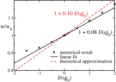
Figure 3: (Color online) The small-current expansion of the width from numerical integration of the Eqs.(22-24) is compared to the phenomenological theory of Subsection IV.3. The width is scaled by its value at $J=0$ while the current is scaled by $qj_{0}$ where $j_{0}$ is the particle flux at $J=0$.

The numerical factor in front of $J/qj_{0}$ is of course a question and this is why we carried out the numerical integration of the differential equations. The equations are simple and the numerics does not pose any problem. Fig.3 shows the comparison of the numerical results with the phenomenological theory. The agreement is surprisingly good in view of the simplicity of the phenomenological arguments we used. Thus our assumptions entering the derivation of $w(J)$ in the small $J$ and large $k$ limits appear to be justified.

V Asymmetric setup

We would like to control the width and so, it is useful to consider a more general case provided by asymmetric boundary condition $a_{0}\not=b_{0}$ since it introduces a new control parameter

$$Q=\frac{b_{0}}{a_{0}}\quad.$$ (48)

The study of this case follows the steps of the symmetric case. First, the point like reaction zone ($k_{0}\to\infty$) is solved exactly, then the phenomenological consideration are repeated, and finally, the numerical simulations are used to check the validity of the phenomenology.

As before, for $k_{0}\to\infty$, the left and the right sides of the front can be treated separately. For the left hand side ($x<x_{f}$) one can use the equations (22), (23) and (24) while for the right hand site ($x>x_{f}$) the equations are as follows

$$(b^{+})^{{}^{\prime\prime}}-J_{0}\left(\frac{b^{+}}{b^{+}+b^{-}+a^{+}}\right)^{\prime}=0\quad$$ (49)

$$(a^{+})^{{}^{\prime\prime}}-J_{0}\left(\frac{a^{+}}{b^{+}+b^{-}+a^{+}}\right)^{\prime}=0\quad$$ (50)

$$(b^{-})^{{}^{\prime\prime}}+J_{0}\left(\frac{b^{-}}{b^{+}+b^{-}+a^{+}}\right)^{\prime}=0\quad,$$ (51)

and the electroneutrality condition for $x>x_{f}$ reads

$$a^{+}+b^{+}-b^{-}=0\quad.$$ (52)

These equations are solved with the following boundary conditions for the dimensionless quantities. At the outer boundaries we have $a^{\pm}(-1/2)=1$, $b^{-}(-1/2)=0$, $a^{+}(1/2)=0$, and $b^{\pm}(1/2)=Q$. At the front ($x=x_{f}$), one has $a^{-}(x_{f})=0,~{}b^{+}(x_{f})=0$ and $a^{+}(x_{f})=b^{-}(x_{f})$. Finally, the conditions for the slopes at $x=x_{f}$ are:

$$\left.(a^{-})^{\prime}\right|_{x_{f}^{-}} = -\left.(b^{+})^{\prime}\right|_{x_{f}^{+}}$$ (53)

$$\left.(a^{+})^{\prime}\right|_{x_{f}^{-}} = \left.(a^{+})^{\prime}\right|_{x_{f}^{+}}$$ (54)

$$\left.(b^{-})^{\prime}\right|_{x_{f}^{-}} = \left.(b^{-})^{\prime}\right|_{x_{f}^{+}}$$ (55)

where $x_{f}^{-}$ ($x_{f}^{+}$) denotes the left (right) side of the reaction zone.

Since the solution of the above problem is similar to the symmetric case (though the algebra is much more tedious), we present only the main results.

Due to asymmetry, the position of the front $x_{f}$ shifts from $x=0$ and one finds that it is given by

$$x_{f} = \frac{1-Q}{2(1+Q)}+\frac{J_{0}}{2Q(1+Q)^{2}}\times$$

$$\left[Q-Q^{2}+\ln\left(\frac{1}{1+Q}\right)-Q^{3}\ln\left(\frac{Q}{1+Q}\right)\right]\;.$$

An important quantity for the phenomenological arguments is the slope of the concentration of the reacting ion $a^{-}$ on the left-hand side of $x_{f}$. It is found to be

$$\left.(a^{-})\right|_{x_{f}}=-(1+Q)+\alpha(Q)J_{0}$$ (57)

with

$$\alpha(Q)=1+\frac{1}{2Q}\ln\left(\frac{1}{1+Q}\right)+\frac{Q}{2}\ln\left(\frac{Q}{1+Q}\right)\,.$$ (58)

Fig. 4 shows the dependence of $\alpha$ on $Q$ and one can observe that $\alpha(Q)$ has a minimum at $Q=1$ i.e. in the symmetric setup. As expected the expression (58) is invariant under the exchange of the boundary concentration values, $a_{0}$ and $b_{0}$, i.e.  $\alpha(Q)=\alpha(1/Q)$.

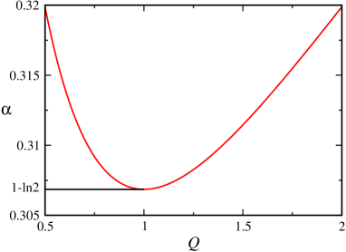
Figure 4: (Color online) $Q$ dependence of the parameter $\alpha$.

For finite reaction rate, one can follow the steps of the phenomenological arguments of the symmetric case, and calculate the first order expansion of $w(J)$ in $J/(qj_{0})$ where $j_{0}$ is given now by

$$j_{0}=(a_{0}+b_{0})D/L\,.$$ (59)

The final result is

$$\frac{w}{w_{0}}=1+\frac{\alpha(Q)}{3}\frac{J}{qj_{0}}$$ (60)

suggesting that the width of the reaction zone is more effectively reduced when the system is asymmetric.

The predictions of the phenomenological arguments can again be compared with the results of a numerical integration of the differential equations. The agreement is qualitatively similar to the symmetric case and the tendency of an increasing impact of the imposed current on the reaction front width when enhancing the asymmetry has been verified.

VI Considerations about the width of a moving front

Although our motivation for this work comes from controlling precipitation patterns which emerge in the wake of a moving reaction-diffusion front ourprl ; encoding , as a first step, we considered the controllability of the width in a simpler stationary state. Clearly, it should be now clarified to what extent the results are generalizable to the case of moving fronts.

The first step in the generalization is the realization that diffusion fronts slow down with time (their velocity is proportional to $1/\sqrt{t}$). This means that the system enters a quasistationary regime where stationary state considerations usually yield correct result. As a relevant example here, let us examine the time evolution of the width of the reaction zone $\tilde{w}_{0}(t)$ emerging when the reagents are initially separated and no current is present [$a(x<0,t=0)=a_{0}$, $b(x<0,t=0)=0$, $a(x>0,t=0)=0$, $b(x>0,t=0)=b_{0}<a_{0}$, $L\to\infty$]. In this case, the front moves diffusively and the width grows with time as zol $\tilde{w}_{0}(t)\sim t^{1/6}$. This time-evolution can be derived easily from the stationary state resultredner $w\sim(D^{2}/kj_{0})^{1/3}$ [see eq.(45)] by the following argument. The width of depletion zone (the region where the concentration profiles are significantly different from their initial values) grows with time as $W_{d}(t)\sim\sqrt{Dt}$. Then the diffusive current towards the reaction zone is obtained as $j_{0}(t)\sim D(a_{0}+b_{0})/W_{d}(t)\sim t^{-1/2}$, and one finds the desired time-evolution as

$$\tilde{w}_{0}(t)\sim\left(\frac{D^{2}}{kj_{0}(t)}\right)^{1/3}\sim t^{1/6}\,.$$ (61)

The second property of the front needed for the generalization is that the motion of the front remains diffusive even if the ionic nature of the reagents are taken into account and a small current is switched on bena . Assuming that the diffusive nature of the front implies quasistationarity, one can go through the estimates of the various terms in the reaction-diffusion equations provided those terms are restricted to the neighborhood (the region of depletion zone) of the reaction front. Using the quasistationary time evolution of the diffusive current $j_{0}\sim t^{-1/2}$, one finds then that the neglected time derivatives are indeed small provided $\tilde{w}(t)\ll W_{d}(t)$. Furthermore, following along the same steps which lead to the estimates of $w/w_{0}$ in the small electric current limit [see the derivations of eqs.(47) and (60) in Sec.IV.3 and Sec.V], one finds

$$\tilde{w}(t)\approx\tilde{w}_{0}(t)\left[1+\tilde{\alpha}\frac{J}{qj_{0}(t)}\right]$$ (62)

where $\tilde{\alpha}$ is a numerical constant of the order one. An important conclusion to be drawn from the above expression is that the direction of the current has the same effect as before. Namely, the forward current decreases the width while the backward current increases it.

Unfortunately, the decrease of $j_{0}\sim t^{-1/2}$ makes it clear that the expansion of $\tilde{w}$ in $J/qj_{0}$ cannot be valid for large times. It is valid only at intermediate times when the quasistationary regime has already set in but the electric current is still smaller than the diffusive current.

Clearly, we cannot claim here that the width of a moving front in the presence of a current has been understood. We believe, however, that the solution should have the properties described above in a well-defined intermediate-time regime. Finally, we should also note that, in the control of precipitation patterns ourprl , one employs actually time-dependent currents and one has some freedom in the design of those current. Consequently, the effects of variable currents on the width, and the use of the freedom in the choice of current to control the width provide additional challenges which should be treated once we arrived at basic understanding of the simpler problems.

VII Discussion and Final remarks

We have studied the effects of an external electric current (or potential difference) on the width of the reaction zone in an irreversible $A^{-}+B^{+}\to C$ reaction-diffusion process. The aim was to find a flexible control of the width since this would help in the attempts of downscaling the patterns generated by reaction-diffusion processes.

Unfortunately, we have to conclude that the width of the reaction zone is not very sensitive to the presence of an externally imposed electric current or potential difference. In the symmetric setup for a typical values $J/qj_{0}$ of order $-1$, the reduction of the width compared to the zero-current case is of the order of 10% at best (see Fig.3) and, furthermore, even a strong asymmetry in the boundary conditions ($Q\to\infty$) allows only a reduction of the order of 20% [see Eqs.(58,60)].

Clearly, the new attempts at control should start now with the reexamination of $w_{0}$. In order to see the problem, let us write Eq.(45) in terms of the characteristic concentration and lengthscale of the system

$$w_{0}\approx\left(\frac{D^{2}}{kj_{0}}\right)^{1/3}\approx\left(\frac{D}{k}\cdot\frac{L}{a_{0}}\right)^{1/3}.$$ (63)

The rate constant $k$ and the diffusion constant $D$ cannot be controlled effectively. So, what remains to consider is the gradient of concentrations, $a_{0}/L$, and one can see from Eq.(63), that small width is obtained by large concentration gradients. Actually, the wet stamping method Grzy1 ; Grzy2 employs large gradients ($a_{0}\approx 1M$ and $L\approx 100\mu$) to achieve patterns with features at submicron scales. The problem with wet stamping, however, is that the patterns are generated by skillfully preparing the boundary conditions and thus the method runs into difficulties with the task of building three-dimensional patterns. Nevertheless, the wet stamping points towards a possible solution of our problem. Namely, we would have to design reaction-diffusion processes which can support large concentration gradients in a reaction zone whose motion can be controlled. Of course, this appears to be a nontrivial task.

Although the diffusion constant $D$ cannot be controlled, one can still think about considering materials where $D$ is significantly different from those of the ions in gels ($D_{gel}\approx 10^{-8}m^{2}/s$). In solid state systems, like for example glasses, the diffusion coefficients differ strongly from the typical values in gelatine materials (typically $D_{solids}\approx 10^{-18}m^{2}/s$) Halle . Accordingly, the zero-current width can be extremely small, since $w(0)\sim D^{2/3}$ (see Eq. (61)).

The study of glassy systems is also interesting since the dynamics of reactants may become subdiffusive in a glassy matrix. For subdiffusive systems we have $D\to 0$ and, as recent studies have shown, the subdiffusive reaction-diffusion dynamics leads to striking changes in the concentration profiles of the reacting ions Sokolov . Thus, combining subdiffusivity with the use of electric currents appears to be a promising way of producing controlled reaction zones of very narrow (submicron) width.

- (1) H. K. Henisch, Periodic precipitation, Pergamon Press, New York (1991).
- (2) E. Kotomin and V. Kuzovkov, Modern Aspects of Diffusion-Controlled Reactions: Cooperative Phenomena in Bimolecular Processes (Elsevier, Amsterdam, 1996).
- (3) D. ben Avraham and S. Havlin, Diffusion and Reactions in Fractals and Disordered Systems (Cambridge University Press, Cambridge, 2000).
- (4) J.D. Murray, Mathematical Biology (Springer Verlag, Berlin, 1990).
- (5) L. Gálfi and Z. Rácz, Phys. Rev. A 38, 3151 (1988).
- (6) F. Leyvraz and S. Redner, Phys. Rev. Lett. 66, 2168 (1991); S. Redner and F. Leyvraz, J. Stat. Phys. 65, 1043 (1991).
- (7) S. Cornell, B. Chopard and M. Droz, Physica A 188, 322-337 (1992).
- (8) S. Cornell and M. Droz, Phys. Rev. Lett. 70, 3824 (1993).
- (9) I. Bena, M. Droz, K. Martens and Z. Racz, J. Phys.: Condens. Matter 19, 065103 (2007).
- (10) E. Ben-Naim and S. Redner, J. Phys. A 25, L575-L583 (1992).
- (11) Y.-E. L. Koo and R. Kopelman, J. Stat. Phys. 65, 893 (1991).
- (12) C. Leger, F. Argoul, and M. Z. Bazant, J. Phys. Chem. B 103, 5841 (1999).
- (13) S. H. Park, S. Parus, R. Kopelman, and H. Taitelbaum, Phys. Rev. E 64, 055102(R) (2001).
- (14) C. N. Baroud, F. Okkels, L. Ménétrier, and P. Tabeling, Phys. Rev. E 67, 060104 (2003).
- (15) S. H. Park, H. Peng, R. Kopelman, and H. Taitelbaum, Phys. Rev. E 75, 026107 (2007).
- (16) See, e.g., I. Rubinstein, Electrodiffusion of Ions (SIAM, Philadelphia, 1990); J. Koryta, J. Dvorak, and L. Kavan, Principles of Electrochemistry (John Wiley & Sons, New York, 1993).
- (17) T. Unger and Z. Rácz, Phys. Rev. E 61, 3583 (2000).
- (18) I. Bena, F. Coppex, M. Droz and Z. Rácz, J. Chem. Phys. 122, 024512 (2005).
- (19) I. Bena, M. Droz, I. Lagzi, K. Martens, Z. Rácz, and A. Volford, Phys. Rev. Lett. 101, 075701, (2008).
- (20) K. Martens, I. Bena, M. Droz and Z. Rácz, J. Stat. Mech. P12003 (2008).
- (21) R. Klajn, M. Fialkowski, I. T. Bensemann, A. Bitner, C. J. Campbell, K. Bishop, S. Smoukov and B. A. Grzybowski, Nat. Mater. 3, 729 (2004).
- (22) I. T. Bensemann, M. Fialkowski, and B. A. Grzybowski, J. Chem. Phys. B 109, 2774 (2005).
- (23) C. Mohr, M. Dubiel and H. Hofmeister, J. Phys. Condensed Matter 13, 525 (2001).
- (24) D. Froemberg and I. M. Sokolov, Phys. Rev. Lett. 100, 108304 (2008).