Gauge Orbits and the Coulomb Potential

Abstract

If the color Coulomb potential is confining, then the Coulomb field energy of an isolated color charge is infinite on an infinite lattice, even if the usual UV divergence is lattice regulated. A simple criterion for Coulomb confinement is that the expectation value of timelike link variables vanishes in Coulomb gauge, but it is unclear how this criterion is related to the spectrum of the corresponding Faddeev-Popov operator, which can be used to formulate a quite different criterion for Coulomb confinement. The purpose of this article is to connect the two seemingly different Coulomb confinement criteria, and explain the geometrical basis of the connection.

I Introduction

The Coulomb potential in non-abelian gauge theories is of interest for several reasons. First of all, since a confining Coulomb potential is a necessary (though not sufficient) condition for having a confining static quark potential Dan , an understanding of the former type of potential could be helpful in understanding the latter, at least in the Casimir-scaling regime. Secondly, the Coulomb potential may be useful in various hadron phenomenology and spectrum calculations, perhaps along the lines suggested by Szczepaniak and co-workers Adam . Finally, the confining Coulomb potential is an important ingredient in the “gluon-chain” model gchain , which is a theory of the formation of color electric flux tubes (for a recent development, see new ).

If there is a confining Coulomb potential, then the Coulomb energy of an isolated color charge in an infinite volume must be infinite, even with a lattice regulation of the usual ultraviolet divergence, and this condition can be expressed in two very different ways. The first, derived in ref. GOZ1 , is obtained from the expectation value of the non-local term in the Coulomb gauge Hamiltonian, and is a condition on the density of near-zero modes of the Faddeev-Popov operator. The second is the criterion that the expectation value of timelike link variables vanishes in Coulomb gauge GOZ2 . These two criteria are so different that they appear to have, at best, only a very indirect relationship. In this article I will show how one criterion depends on the other, and discuss the relevant properties of gauge orbits which underlie this dependency.

It is important to first understand where these two different Coulomb confinement criteria come from. Consider the physical state

$$\Psi^{a}_{q}=q^{a}({\mathbf{x}})\Psi_{0}$$ (1)

in Coulomb gauge, where $q^{a}$ is a heavy quark operator, and $\Psi_{0}$ is the ground state. Let

$$T=\exp[-(H-E_{0})a]$$ (2)

represent the lattice theory transfer matrix, divided by a factor of $\exp(-E_{0}a)$, where $E_{0}$ is the vacuum energy and $a$ is the lattice spacing. Then

$$\exp[-E_{self}] \equiv \langle\Psi^{a}_{q}|T|\Psi^{a}_{q}\rangle$$ (3)

$$= \langle\text{Tr}[U_{0}({\mathbf{x}},t)]\rangle$$

$$\rightarrow 0$$

where $E_{self}$ is the Coulomb energy, in lattice units, of the isolated heavy quark state, and the last line holds if this self-energy is infinite in an infinite volume (with the UV divergence controlled by the finite lattice spacing). This means that Coulomb confinement, on the lattice, is equivalent to having a vanishing expectation value for the trace of timelike link variables. It was noted long ago that Coulomb gauge does not fix the gauge completely; there is a remnant gauge symmetry which depends on time but is homogenous in space:

$$U_{i}({\mathbf{x}},t) \rightarrow g(t)U_{i}({\mathbf{x}},t)g^{\dagger}(t)$$

$$U_{0}({\mathbf{x}},t) \rightarrow g(t)U_{0}({\mathbf{x}},t)g^{\dagger}(t+1)$$ (4)

If remnant gauge symmetry is unbroken, then $\langle\text{Tr}[U_{0}]\rangle=0$ Parisi , and the Coulomb energy of an isolated color charge is infinite GOZ2 .

On the other hand, the Coulomb energy of an isolated charge can alternatively be expressed in terms of the inverse Faddeev-Popov operator:

$$E_{self}={\texttt{g}^{2}C_{F}\over N^{2}-1}\Bigl{\langle}(M^{-1}(-\nabla^{2})M^{-1})_{{\mathbf{x}}{\mathbf{x}}}^{aa}\Bigl{\rangle}$$ (5)

where $C_{F}$ is the quadratic Casimir of the fundamental representation of the SU(N) gauge group, g is the gauge coupling, and

$$M^{ab}_{{\mathbf{x}}{\mathbf{y}}}[A]=-(\nabla\cdot D^{ab})_{{\mathbf{x}}}\delta({\mathbf{x}}-{\mathbf{y}})$$ (6)

is the Faddeev-Popov (F-P) operator, with $D_{k}^{ab}$ the covariant derivative. Let $\{\lambda_{n},\phi_{n}^{a}(x)\}$ denote the set of eigenvalues and eigenstates of the F-P operator

$$M^{ab}_{{\mathbf{x}}{\mathbf{y}}}\phi^{b}_{n}({\mathbf{y}})=\lambda_{n}\phi^{a}_{n}({\mathbf{x}})$$ (7)

Then it is fairly straightforward to show that in an infinite volume, where the spectrum of $M$ is continuous, we have GOZ1

$$E_{self}\propto\texttt{g}^{2}\int_{0}^{\lambda_{max}}d\lambda~{}\left\langle\rho(\lambda){(\phi_{\lambda}|(-\nabla^{2})|\phi_{\lambda})\over\lambda^{2}}\right\rangle$$ (8)

where $\rho(\lambda)$ is the density of eigenvalues, normalized to unity. Coulomb confinement ($E_{self}=\infty$) requires that integral in (8) diverges from a singularity in the integrand at the lower limit, due to the near-zero eigenmodes. The existence of such eigenmodes implies that the Coulomb gauge lattice configuration, in an infinite volume, lies at the Gribov horizon, in accordance with the Gribov-Zwanziger scenario Dan1 . However, while proximity to the horizon is certainly a necessary condition for Coulomb confinement, it is not sufficient. The density and behavior of near-zero eigenmodes must also be such that the integral in eq. (8) is divergent.

We therefore have two, apparently quite distinct, criteria for Coulomb confinement:

A) $$\qquad\lim_{\lambda\rightarrow 0}{\left\langle\rho(\lambda)(\phi_{\lambda}|(-\nabla^{2})|\phi_{\lambda})\right\rangle\over\lambda}>0$$ (9)

B) $$\qquad\langle\text{Tr}[U_{0}({\mathbf{x}},t)]\rangle=0$$ (10)

These conditions look very different. They are, in fact, associated with two different ways of computing the Coulomb potential. The first is to calculate the potential

$$V_{C}(R)=-\texttt{g}^{2}C_{F}{1\over N^{2}-1}\Bigl{\langle}[M^{-1}(-\nabla^{2})M^{-1}]^{aa}_{{\mathbf{x}}{\mathbf{y}}}\Bigr{\rangle}$$ (11)

directly, on the lattice, and a number of authors have followed this approach direct . The published results provide data for the Coulomb potential in momentum space, which appears to go as $1/k^{4}$ at small $k$. A second, and computationally much simpler method was suggested in ref. GO , and only requires computing the correlators of timelike link variables, in Coulomb gauge, at equal times. Define

$$\Psi_{q\overline{q}}=\overline{q}^{a}(0)q^{a}(R)\Psi_{0}$$ (12)

and let $a_{t}=\xi a$ be the lattice spacing in the time direction. Then

$$\exp[-\xi{\cal E}(R)] \equiv \langle\Psi_{q\overline{q}}|T|\Psi_{q\overline{q}}\rangle$$ (13)

$$= \langle\Psi_{q\overline{q}}|e^{-(H-E_{0})a_{t}}|\Psi_{q\overline{q}}\rangle$$

$$= \langle\text{Tr}[U_{0}^{\dagger}({\mathbf{x}},t)U_{0}({\mathbf{y}},t)]\rangle$$

so that the Coulomb energy ${\cal E}(R)$ associated with a static $q\overline{q}$ state, in units of the spatial lattice spacing $a$, is given by the timelike link-link correlator

$${\cal E}(R) = -{1\over\xi}\log\Bigl{[}\langle\text{Tr}[U_{0}^{\dagger}({\mathbf{x}},t)U_{0}({\mathbf{y}},t)]\rangle\Bigr{]}$$ (14)

$$= V_{C}(R)+\text{const}$$

where $R=|{\mathbf{x}}-{\mathbf{y}}|$. This approach has been followed (at $\xi=1$) in refs. GO ; japan . The Coulomb string tension $\sigma_{C}$ is extracted from the exponential falloff of the timelike link-link correlator

$$\langle\text{Tr}[U_{0}^{\dagger}({\mathbf{x}},t)U_{0}({\mathbf{y}},t)]\rangle\sim e^{-\xi\sigma_{C}R}$$ (15)

and of course this exponential falloff is only possible if condition B (eq. (10) above) is satisfied. The interesting question is why $\langle\text{Tr}[U_{0}]\rangle=0$, and how this condition is related to the Coulomb confinement criterion A (eq. (9)), which is formulated in terms of the spectrum of the F-P operator.

II Gauge orbits and their near-tangential intersections

The suggestion I will make here is that the condition $\langle\text{Tr}[U_{0}]\rangle=0$, and the existence of a finite correlation length among timelike link variables, is associated with the way in which a typical gauge orbit intersects the submanifold of gauge fields satisfying the Coulomb gauge condition, and that this in turn is related to the density of near-zero F-P eigenmodes. In continuum notation, let $A_{k}^{a}({\mathbf{x}})$ represent a gauge field at some fixed time $t$ (spatial index $k=1,2,3$), and

$$F^{a}_{\mathbf{x}}[A]\equiv\nabla\cdot{\bf A}^{a}({\mathbf{x}})=0$$ (16)

is the Coulomb gauge condition. The Fadeev-Popov (F-P) operator $M$ is given by

$$M^{ab}_{xy}[A] = -\texttt{g}\left({\delta\over\delta\theta^{b}({\mathbf{y}})}F^{a}_{\mathbf{x}}[g\circ A]\right)_{|_{\theta=0}}$$ (17)

$$= -\partial_{k}D^{ab}_{k}\delta({\mathbf{x}}-{\mathbf{y}})$$

where

$$g({\mathbf{x}})=\exp[i\theta^{a}({\mathbf{x}})T_{a}]$$ (18)

is a gauge transformation.

Let ${\cal C}$ represent the hypersurface, in the space of gauge fields $A_{k}({\mathbf{x}})$ in $D=3$ dimensions, satisfying the gauge condition condition (16). For a given $A^{\prime}\in{\cal C}$, the corresponding $\{\phi_{n}\}$ can be thought of as a set of orthonormal unit vectors which span the tangent space, at the point $g({\mathbf{x}})=\mathbbm{1}$, of the space of all gauge transformations. Since the gauge orbit $O[A^{\prime}]$ consists of the set of all configurations $g\circ A^{\prime}$, the $\{\phi_{n}\}$ also map to a set of directions spanning the tangent space of the gauge orbit, at the point $A^{\prime}\in{\cal C}$.

It was found in ref. GOZ1 that for typical (i.e. Monte-Carlo generated) lattices, transformed to Coulomb gauge, there is a very large number of near-zero modes with $\lambda_{n}\ll 1$, at least as compared to the corresponding spectrum of the free-field operator $-\delta^{ab}\nabla^{2}$, and this number grows linearly with the lattice volume. Near zero-modes have a geometrical intepretation: these are “flat” directions on the gauge orbit at point $A$, which are nearly tangential to ${\cal C}$. Said in another way: a great many directions on ${\cal C}$ run nearly parallel to the gauge orbits.

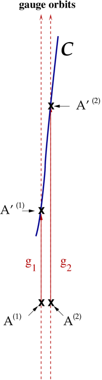
Figure 1: If the gauge-fixing hypersurface ${\cal C}$ defined by $\nabla\cdot A=0$ is almost tangential to many directions on a typical gauge orbit, then the gauge transformations $g_{1}$ and $g_{2}$ which take two nearby configurations $A^{(1)}$ and $A^{(2)}$ into Coulomb gauge may be very different.

To understand the implications of this fact, let us consider two points $A_{k}^{a}({\mathbf{x}})$ and $A_{k}^{a}({\mathbf{x}})+\delta A_{k}^{a}({\mathbf{x}})$ with an infinitesimal separation $\delta A$ in the space of all three-dimensional gauge field configurations (a time slice of the $D=4$ configurations, ignoring the $A_{0}$ component). Let $g_{1}$ and $g_{2}$ be the gauge transformations which bring $A^{(1)}=A$ and $A^{(2)}=A+\delta A$, respectively, onto ${\cal C}$ (Fig. 1) . Of course, $g_{1}$ and $g_{2}$ are not unique because of Gribov copies, and also because of the remnant global gauge symmetry (4) allowed by Coulomb gauge. However, for a given $g_{1}$ the ambiguity in $g_{2}$ can be eliminated by the requirement that $g_{2}$ brings $g_{2}\circ(A+\delta A)$ as close as possible to $g_{1}\circ A$. Then for $\delta A$ infinitesimal, the deviation of $g_{2}$ from $g_{1}$ must also be infinitesimal, and we can write

$$g_{2}({\mathbf{x}})=\exp[i\delta\theta^{a}({\mathbf{x}})T_{a}]g_{1}({\mathbf{x}})$$ (19)

where $T_{a}={\textstyle{\frac{1}{2}}}\sigma_{a}$ for the SU(2) group used below. The deviation $\delta\theta$ is determined from the condition that

$$F^{a}_{x}\Bigl{[}g_{2}\circ(A+\delta A)\Bigr{]}=0$$ (20)

Expanding this condition to first order in a functional Taylor series, and taking account of $F[g_{1}\circ A]=0$, we have

$${\delta F^{a}_{\mathbf{x}}\over\delta(\delta\theta^{b}({\mathbf{y}}))}\delta\theta^{b}({\mathbf{y}})+{\delta F^{a}_{\mathbf{x}}\over\delta(\delta A_{k}^{b}({\mathbf{y}}))}\delta A_{k}^{b}({\mathbf{y}})=0$$ (21)

where repeated indices are summed, repeated coordinates (${\mathbf{y}}$) are integrated, and the functional derivatives are evaluated at $\delta\theta=\delta A=0$. Then, from eq. (17),

$$M^{ab}_{{\mathbf{x}}{\mathbf{y}}}[g_{1}\circ A]\delta\theta^{b}({\mathbf{y}})=\texttt{g}\delta f^{a}({\mathbf{x}})$$ (22)

where

$$\delta f^{a}({\mathbf{x}}) \equiv {\delta F^{a}_{\mathbf{x}}\over\delta A_{k}^{b}({\mathbf{y}})}\delta A_{k}^{b}({\mathbf{y}})$$ (23)

$$= \partial_{k}\Bigl{\{}{\textstyle{\frac{1}{2}}}\text{Tr}[g_{1}({\mathbf{x}})\sigma_{b}g_{1}^{\dagger}({\mathbf{x}})\sigma_{a}]\delta A^{b}_{k}({\mathbf{x}})\Bigr{\}}$$

Now let $\{\phi_{n}\}$ be the eigenstates of the F-P operator $M$ at $g_{1}\circ A$, and expand

$$\delta\theta^{a}({\mathbf{x}}) = \sum_{n>3}\delta\theta_{n}~{}\phi_{n}^{a}({\mathbf{x}})$$

$$\delta f^{a}({\mathbf{x}}) = \sum_{n>3}\delta f_{n}~{}\phi_{n}^{a}({\mathbf{x}})$$

$$M^{ab}_{{\mathbf{x}}{\mathbf{y}}} = \sum_{n>3}\lambda_{n}\phi^{a}_{n}({\mathbf{x}})\phi^{b*}_{n}({\mathbf{y}})$$ (24)

The restriction to $n>3$ in the above summations has to do with remnant global gauge symmetry in Coulomb gauge. For the SU(2) gauge group, the F-P operator has three exact zero modes ($\lambda_{1-3}=0$) on a finite volume with periodic boundary conditions, corresponding to the fact that if a configuration $A$ satisfies the Coulomb gauge condition, so does $g\circ A$ for a spatially independent (i.e. global) gauge transformation. For this reason, the coefficients $\delta\theta_{1-3}$ are not determined by the condition (20), and can be set to anything we choose; in particular they can be set to zero. Note also that $\delta f_{1-3}=0$. This is because the three zero modes are constant in space, while $\delta f({\mathbf{x}})$ is a total derivative, so the inner product of $(\phi_{n}|\delta f)$ vanishes for $n=1,2,3$.

Substituting the expansions (24) into (22), we find for all $n>3$ that

$$\delta\theta_{n}=\texttt{g}{\delta f_{n}\over\lambda_{n}}$$ (25)

This equation takes us to the crux of the matter. The $\delta f_{n}$ coefficients depend on $\delta A_{k}^{a}({\mathbf{x}})$, which is small but otherwise arbitrary, so near-zero $\lambda_{n}$ correspond in general to very large $\delta\theta_{n}$. If there are only a few near-zero eigenmodes, then the few large $\delta\theta_{n}$ may not contribute very much to $\delta\theta({\mathbf{x}})$. On the other hand, if there are a large number of near-zero eigenmodes, then $\delta\theta({\mathbf{x}})$ may also be large, and the deviation between $A^{(1)}$ and $A^{(2)}$ will be greatly magnified upon gauge-fixing to ${\cal C}$, as illustrated in Fig. 1.

The quantity to consider is the mean-square value of $\delta\theta({\mathbf{x}})$, which is given by

$$\overline{|\delta\theta|}^{2} = {1\over V_{3}}\int d^{3}x~{}\delta\theta^{a}({\mathbf{x}})\delta\theta^{a}({\mathbf{x}})$$ (26)

$$= {1\over V_{3}}\sum_{n}\delta\theta_{n}^{2}$$

$$\stackrel{{\scriptstyle V_{3}\rightarrow\infty}}{{\longrightarrow}} \int d\lambda~{}\rho(\lambda)\delta\theta_{\lambda}^{2}$$

$$= \texttt{g}^{2}\int d\lambda~{}{\rho(\lambda)[\delta f(\lambda)]^{2}\over\lambda^{2}}$$

where

$$\delta f(\lambda)=\int d^{3}x~{}\phi^{a*}_{\lambda}({\mathbf{x}})\partial_{k}\text{Tr}[g_{1}\delta A_{k}g_{1}^{\dagger}\sigma_{a}]$$ (27)

and $V_{3}$ is the three-volume of a time-slice. Let us consider the magnitude of $\overline{|\delta\theta|}^{2}$ for a “typical” $\delta A$. To derive this quantity, we need to average over the $\delta A$ with some reasonable, gauge-invariant probability measure. The simplest is a gaussian measure

$$\langle Q[\delta A]\rangle_{gauss}$$

$$= {\int D\delta A~{}Q[\delta A]\exp\left[-{1\over 2\epsilon}\int d^{3}x~{}\delta A^{a}_{k}({\mathbf{x}})\delta A^{a}_{k}({\mathbf{x}})\right]\over\int D\delta A~{}\exp\left[-{1\over 2\epsilon}\int d^{3}x~{}\delta A^{a}_{k}({\mathbf{x}})\delta A^{a}_{k}({\mathbf{x}})\right]}$$

where $\epsilon$ is an infinitesimal constant. In this measure

$$\langle\delta A_{i}^{a}({\mathbf{x}})\delta A_{j}^{b}({\mathbf{y}})\rangle_{gauss}=\epsilon\delta_{ij}\delta^{ab}\delta^{3}({\mathbf{x}}-{\mathbf{y}})$$ (29)

Then

$$\langle\overline{|\delta\theta|}^{2}\rangle_{gauss}$$ (30)

$$= \texttt{g}^{2}\int d\lambda~{}{\rho(\lambda)\over\lambda^{2}}\int d^{3}xd^{3}y\Bigl{\langle}{\textstyle{\frac{1}{4}}}(\partial^{i}_{x}\phi^{a*}_{\lambda}({\mathbf{x}}))\text{Tr}[g_{1}({\mathbf{x}})\sigma_{b}g_{1}^{\dagger}({\mathbf{x}})\sigma_{a}]$$

$$\qquad\delta A^{b}_{i}({\mathbf{x}})\text{Tr}[g_{1}({\mathbf{y}})\sigma_{c}g_{1}^{\dagger}({\mathbf{y}})\sigma_{d}]\delta A^{c}_{j}({\mathbf{y}})(\partial^{j}_{y}\phi^{d}_{\lambda}({\mathbf{y}}))\Bigr{\rangle}_{gauss}$$

$$= \epsilon\texttt{g}^{2}\int d\lambda~{}{\rho(\lambda)(\phi_{\lambda}|(-\nabla^{2})|\phi_{\lambda})\over\lambda^{2}}$$

The above expression still depends on the initial choice of $A$, since the F-P eigenmodes are evaluated at $g_{1}\circ A$, but if we now take the vacuum expectation value, then the integral is precisely the same as the integral that appears in the expression for the Coulomb energy of an isolated charge, shown in eq. (8).

There are now two possible scenarios, depending on whether or not the Coulomb confinement criterion A (eq. (9)) is satisfied. Let

$$G({\mathbf{x}})\equiv\exp[i\delta\theta^{a}({\mathbf{x}})T_{a}]=g_{2}({\mathbf{x}})g_{1}^{\dagger}({\mathbf{x}})$$ (31)

serve to quantify the deviation between gauge transformations $g_{1}$ and $g_{2}$. Making use of the global remnant symmetry (4), it is always possible to set $G({\mathbf{x}})=\mathbbm{1}$ at one particular site ${\mathbf{x}}={\mathbf{x}}_{0}$. If there is no Coulomb confinement, so the integral in (30) is finite, then $\delta\theta({\mathbf{x}})$ is everywhere small for sufficiently small $\delta A$. This means that $G({\mathbf{x}})\approx\mathbbm{1}$ and $g_{2}({\mathbf{x}})\approx g_{1}({\mathbf{x}})$ everywhere in space. On the other hand, if the Coulomb confinement condition A is satisfied, a quite different scenario is possible. It can then happen that no matter how small the magnitude of $\delta A$, the non-compact variable $\delta\theta({\mathbf{x}})$ becomes large at sufficiently large $|{\mathbf{x}}-{\mathbf{x}}_{0}|$, and $\delta\theta$ is a random variable because $\delta A$ is a random variable. In this case, the most likely behavior is that as ${\mathbf{x}}$ varies, $G({\mathbf{x}})$ wanders over the entire group manifold, averaging to zero in an infinite volume. Assuming that $G({\mathbf{x}})$ averages to zero, a better measure of the $g_{1,2}$ deviation is provided by the correlation length among the $G({\mathbf{x}})$, extracted from the correlator

$$D(R)={1\over V_{3}}\int d^{3}x{\textstyle{\frac{1}{2}}}\text{Tr}[G({\mathbf{x}})G^{\dagger}({\mathbf{x}}+{\bf R})]$$ (32)

rather than $G({\mathbf{x}})$ itself. In particular, if $D(R)$ goes as

$$D(R)\sim e^{-\mu R}$$ (33)

at large $R$, then there is a finite correlation length $l_{g}=\mu^{-1}$, and $\langle G\rangle=0$. As $\delta A\rightarrow 0$ (so $g_{2}\rightarrow g_{1}$), we would expect this correlation length to go to infinity, i.e. $\mu\rightarrow 0$. Confinement criterion A is a necessary condition for this kind of behavior, but since eq. (21) is not necessarily valid for $\delta\theta\sim O(1)$, we must resort, in this case, to a numerical investigation.

To summarize: Near-zero modes of the F-P operator correspond to directions in the gauge orbit $O[A]$ which are nearly tangential to the gauge-fixed hypersurface ${\cal C}$, at the point where $O[A]$ intersects $C$. Large numbers of tangential directions should have the following consequence: if $A$ is a typical gauge field on a time slice, and $A+\delta A$ is a nearby configuration on the same timeslice, then the gauge transformations $g_{1}$ and $g_{2}$ which take $A$ and $A+\delta A$ into Coulomb gauge will be wildly different, even for relatively small $\delta A$. More concretely, in theories where the Coulomb energy of an isolated color charge is infinite, eq. (30) suggests that $G({\mathbf{x}})=g_{2}({\mathbf{x}})g^{\dagger}_{1}({\mathbf{x}})$ is a random variable ($\langle G({\mathbf{x}})\rangle=0$) with a finite $GG$ correlation length. On the lattice it is possible to test this possibility, by calculating $D(R)$ numerically.

III Numerical Results

We begin by generating, via lattice Monte Carlo simulations, a set of thermalized SU(2) lattices, using the usual Wilson action in $D=4$ dimensions at $\beta=2.2$. Take any time slice of such a lattice, and denote the link variables as $U^{(1)}_{k}({\mathbf{x}})$. The configuration is fixed to Coulomb gauge by the over-relaxation method, and the gauge transformation (a product of the transformations obtained at each over-relaxation sweep) taking $U^{(1)}$ to Coulomb gauge is denoted $g_{1}({\mathbf{x}})$. Next we construct a “nearby” lattice $U^{(2)}_{k}({\mathbf{x}})$ by adding a small amount of noise to each link variable in the original (non-gauge fixed) $U^{(1)}$, i.e.

$$U^{(2)}_{k}({\mathbf{x}})=\rho_{k}({\mathbf{x}})U^{(1)}_{k}({\mathbf{x}})$$ (34)

where $\rho_{k}({\mathbf{x}})$ is a stochastic SU(2)-valued “noise” field, biased towards the identity, and generated independently at each link with probability distribution

$$\text{prob.\ measure}\propto\exp\Bigl{[}\kappa{\textstyle{\frac{1}{2}}}\text{Tr}(\rho)\Bigr{]}d\rho$$ (35)

where $d\rho$ is the Haar measure. With this probability measure, the average value of $\text{Tr}(\rho)$ as a function of $\kappa$ is

$$\overline{\text{Tr}[\rho]}={I_{2}(\kappa)\over I_{1}(\kappa)}$$ (36)

Having generated $U^{(2)}$ in this way, we fix it to Coulomb gauge by the same over-relaxation procedure that was applied to $U^{(1)}$, and obtain $g_{2}({\mathbf{x}})$. From this we construct $G({\mathbf{x}})=g_{2}({\mathbf{x}})g^{\dagger}_{1}({\mathbf{x}})$, and obtain, on a lattice of extension $L$ in the spatial directions, the correlator

$$D(R)={1\over L^{3}}\sum_{{\mathbf{x}}}\text{Tr}[G({\mathbf{x}})G^{\dagger}({\mathbf{x}}+{\mathbf{R}})]$$ (37)

The final step is to average the values of $D(R)$ obtained on every time-slice of every lattice of a set of independent, thermalized lattices. The result, for average Tr($\rho$)=0.75 ($\kappa=5.67$) and a variety of $L^{4}$ lattice volumes, is shown in Fig. 2. It is clear that $D(R)$ does indeed fall off exponentially, with inverse correlation length $\mu=0.30$.

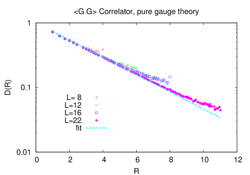
Figure 2: The gauge transformation correlator $D(R)$ vs. $R$. The correlator is evaluated, at various $L^{4}$ lattice volumes, for configurations $U^{(1)}$ generated by lattice Monte Carlo in SU(2) pure gauge theory at $\beta=2.2$, and $U^{(2)}$ derived from $U^{(1)}$ with noise parameter $\kappa=5.67$ (${\textstyle{\frac{1}{2}}}\overline{\text{Tr}(\rho)}=0.75$). The straight line is a fit of $\exp(-\mu R)$ to the data at low $R$.

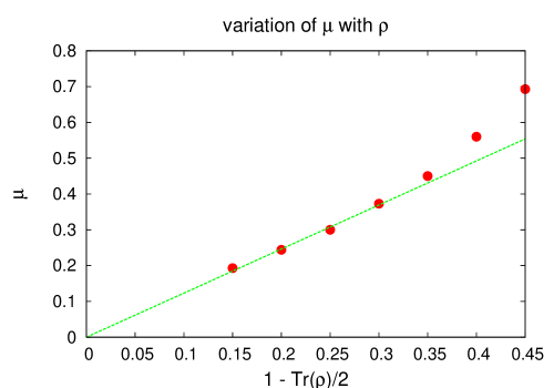
Figure 3: Inverse correlation length $\mu$, extracted from $D(R)$ calculated for various values of the noise parameter $\kappa$, corresponding to ${\textstyle{\frac{1}{2}}}\text{Tr}(\rho)$ in the range $0.55-0.85$. Errorbars are smaller than the symbol size. The straight line is a fit to the first four data points.

As $\kappa\rightarrow\infty$ and $\text{Tr}(\rho)\rightarrow 1$, it must be that the inverse correlation length $\mu$ goes to zero. Fig. 3 is a plot of $\mu$ vs. average $\text{Tr}(\rho)$. For lattice configurations $U^{(1)}$ generated (without gauge fixing) at $\beta=2.2$, the results are consistent with

$$\mu=c\Bigl{(}1-{\textstyle{\frac{1}{2}}}\overline{\text{Tr}[\rho]}\Bigr{)}$$ (38)

and $c=1.23$, as the average $\text{Tr}[\rho]\rightarrow 1$. On a finite lattice (the maximum size used here is $L^{4}=22^{4}$), the practical constraint on $\kappa$ is that it should not be so large that finite size effects are dominant. Note also that $g_{2}\rightarrow g_{1}$ only for $U^{(2)}$ approaching $U^{(1)}$, rather than approaching some arbitrary gauge copy of $U^{(1)}$. If, e.g., $U^{(2)}$ is taken to be a random gauge copy of $U^{(1)}$, and the $U^{(1,2)}$ are transformed via over-relaxation to Coulomb gauge, then the gauge-fixed configurations are, in general, Gribov copies of one another. Numerically it is found that $D(R)$ is consistent with zero in this case, for all $R>0$.

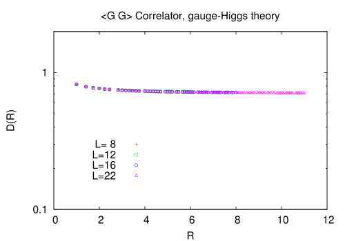
Figure 4: Same as Fig. 2, except that the $U^{(1)}$ are generated from lattice Monte Carlo simulation of SU(2) gauge-Higgs theory (eq. (39)), in the Higgs-like region at couplings $\beta=2.2,~{}\gamma=1.2$. Noise parameter $\kappa=5.67$ is the same as in Fig. 2.

Finally, since the conjecture is that $\langle G\rangle=0$ results from a high density of near-zero F-P eigenvalues, as compared to the density in a free field or non-confining theory, we should find, conversely, that (i) $\langle G\rangle\neq 0$; and (ii) $D(R)$ has a non-zero limit as $R\rightarrow\infty$; when $G({\mathbf{x}})$ is evaluated for field configurations $U^{(1)}$ which do not have this high density of near-zero F-P eigenvalues. More precisely, we expect $\langle G\rangle\neq 0$ for configurations in which the rhs of (26) is finite in the infinite volume limit. Such configurations can be generated, e.g., by center vortex removal in confining lattices, or alternatively by Monte Carlo simulation of an SU(2) gauge-Higgs theory

$$S=\beta\sum_{plaq}{\textstyle{\frac{1}{2}}}\text{Tr}[U(P)]+\gamma\sum_{x,\mu}{\textstyle{\frac{1}{2}}}\text{Tr}[\varphi^{\dagger}({\mathbf{x}})U_{\mu}({\mathbf{x}})\varphi(x+\widehat{\mu})]$$ (39)

in the “Higgs-like” region of parameter space. Here $U(P)$ denotes one-plaquette loops, and $\varphi({\mathbf{x}})$ is an SU(2) matrix-valued Higgs field. It was shown in GOZ1 that the eigenvalue densities are qualitatively very similar in vortex-removed and gauge-Higgs configurations, and are essentially a perturbation of the free field result. The result for $D(R)$ in a gauge-Higgs theory at $\beta=2.2,~{}\texttt{g}=1.2$ is shown in Fig. 4. Here we see that $D(R)$ does not have an exponential falloff; in fact it appears to approach a limiting value. Hence $\mu=0$ and $\langle G\rangle\neq 0$ in this case, as expected.

IV Coulomb confinement

It is time to return to the question posed in the Introduction: how do near-zero F-P eigenmodes enforce $\langle\text{Tr}[U_{0}]\rangle=0$, which implies Coulomb confinement?

Consider a Monte Carlo simulation carried out in temporal gauge, with asymmetry parameter $\xi$. The SU(2) Wilson action is given by

$$S = {\beta\over\xi}\sum_{{\mathbf{x}},t}\sum_{k=1}^{3}{\textstyle{\frac{1}{2}}}\text{Tr}[U_{k}({\mathbf{x}},t)U^{\dagger}_{k}({\mathbf{x}},t+1)]$$

$$+ \beta\xi\sum_{{\mathbf{x}},t}\sum_{i<j}{\textstyle{\frac{1}{2}}}\text{Tr}[U_{i}({\mathbf{x}},t)U_{j}({\mathbf{x}}+\widehat{e}_{i},t)U^{\dagger}_{i}({\mathbf{x}}+\widehat{e}_{j},t)U^{\dagger}_{j}({\mathbf{x}},t)]$$

Suppose that $\xi\ll 1$. In that case, the first term in the action will require that link variables $U_{k}({\mathbf{x}},t)$ and $U_{k}({\mathbf{x}},t+1)$ are almost identical. This means that we may think of the sets of link variables at fixed times $t$ and $t+1$ as being an instance of “nearby” $D=3$ dimensional lattice configurations $U^{(1)}$ and $U^{(2)}$. In fact, writing

$$U_{k}({\mathbf{x}},t+1)=\eta_{k}({\mathbf{x}},t)U_{k}({\mathbf{x}},t)$$ (41)

the lattice action has the form

$$S={\beta\over\xi}\sum_{{\mathbf{x}},t}\sum_{k=1}^{3}{\textstyle{\frac{1}{2}}}\text{Tr}[\eta_{k}({\mathbf{x}},t)]+\beta\xi\sum_{{\mathbf{x}},t}\sum_{i<j}{\textstyle{\frac{1}{2}}}\text{Tr}[U(P_{ij}({\mathbf{x}},t))]$$

where $U(P_{ij}({\mathbf{x}},t))$ is a loop around the space-like plaquette $P_{ij}({\mathbf{x}},t)$. Then, if $Q$ is any functional of the $\eta_{k}({\mathbf{x}},t)$ at fixed $t$,

$$\langle Q\rangle = \int DU(t+1)DU(t)~{}\Psi^{*}_{0}\Bigl{[}U(t+1)\Bigr{]}Q[\eta(t)]\exp\left[{\beta\over\xi}\sum_{{\mathbf{x}}}\sum_{k=1}^{3}{\textstyle{\frac{1}{2}}}\text{Tr}[\eta_{k}({\mathbf{x}},t)]+\xi\beta\times\text{space-like plaquettes}\right]\Psi_{0}\Bigl{[}U(t)\Bigr{]}$$ (43)

$$= \int D\eta(t)DU(t)~{}\Psi_{0}^{*}\Bigl{[}\eta(t)U(t)\Bigr{]}\Psi_{0}\Bigl{[}U(t)\Bigr{]}Q[\eta(t)]\exp\left[{\beta\over\xi}\sum_{{\mathbf{x}}}\sum_{k=1}^{3}{\textstyle{\frac{1}{2}}}\text{Tr}[\eta_{k}({\mathbf{x}},t)]+\xi\beta\times\text{space-like plaquettes}\right]$$

where $\Psi_{0}[U]$ is the ground state (i.e. lowest energy eigenstate of the transfer matrix) in temporal gauge. For $\xi\ll 1$ we have, to leading order in $\xi$,

$$\langle Q\rangle=\int D\eta(t)~{}Q[\eta(t)]\exp\left[{\beta\over\xi}\sum_{{\mathbf{x}}}\sum_{k=1}^{3}{\textstyle{\frac{1}{2}}}\text{Tr}[\eta_{k}({\mathbf{x}},t)]\right]$$ (44)

So to leading order there are no correlations between the $\eta_{k}({\mathbf{x}},t)$ at different lattice sites, and the probability measure for $\eta_{k}({\mathbf{x}})$ at a given link $k,{\mathbf{x}}$ is simply

$$\text{prob. measure}\propto\exp\left[{\beta\over\xi}{\textstyle{\frac{1}{2}}}\text{Tr}[\eta]\right]d\eta$$ (45)

where $d\eta$ is the Haar measure. Identifying $\kappa=\beta/\xi$, this is exactly the same as the probability measure for the noise variable $\rho$ of the previous section, and for $\xi\ll 1$ it is strongly biased towards the identity. Therefore, $U^{(1)}=\{U_{k}({\mathbf{x}},t)\}$ and $U^{(2)}=\{U_{k}({\mathbf{x}},t+1)\}$ are close together in the space of $D=3$ lattice configurations.

Now to compute the Coulomb potential, we transform the temporal gauge lattice configurations to Coulomb gauge via, e.g., over-relaxation. These transformations can be computed independently at each time slice. Pick any time $t$, and denote

$$U^{C}_{k}({\mathbf{x}},t) = g_{1}({\mathbf{x}})U_{k}({\mathbf{x}},t)g_{1}^{\dagger}({\mathbf{x}}+{\bf e}_{k})$$

$$U^{C}_{k}({\mathbf{x}},t+1) = g_{2}({\mathbf{x}})U_{k}({\mathbf{x}},t+1)g_{2}^{\dagger}({\mathbf{x}}+{\bf e}_{k})$$ (46)

where the “C” superscript indicates the link variables transformed to Coulomb gauge, with $g_{1}$ and $g_{2}$ the gauge transformations which take the temporal gauge lattices, at times $t$ and $t+1$ respectively, into Coulomb gauge. Then the timelike link variables at time $t$ are simply a product of these tranformations, i.e.

$$U^{C}_{0}({\mathbf{x}},t) = g_{1}({\mathbf{x}})g_{2}^{\dagger}({\mathbf{x}})$$ (47)

$$= G^{\dagger}({\mathbf{x}})$$

But this means that

$$\langle\mbox{Tr}[U_{0}({\mathbf{x}},t)]\rangle=\langle\mbox{Tr}[G({\mathbf{x}})]\rangle$$ (48)

and also, referring back to eq. (14), that

$$V_{C}(R)=-\xi^{-1}\log\Bigl{[}\langle\text{Tr}[G({\mathbf{x}})G^{\dagger}({\mathbf{x}}+{\bf R})]\rangle\Bigr{]}-\text{const.}$$ (49)

The conclusion is that the property $\langle G\rangle=0$, which requires that Coulomb confinement condition A (eq. (9)) is satisfied, in turn implies Coulomb confinement condition B, i.e. $\langle U^{C}_{0}\rangle=0$. The latter condition also tells us that remnant global gauge symmetry in Coulomb gauge, shown in eq. (4), is unbroken (cf. the discussion in ref. GOZ2 on this point). Moreover, a finite correlation length among the $G({\mathbf{x}})$ implies a linear Coulomb potential.

In the notation of the previous section, $G({\mathbf{x}})=\exp[i\delta\theta({\mathbf{x}})]$, and from eq. (47), we see that when $G({\mathbf{x}})$ is obtained from temporal gauge, $\delta\theta^{a}$ plays the role of $g\xi A_{0}^{a}({\mathbf{x}})$. It must be stressed, however, that while we can obtain $U_{0}^{C}$ by exponentiating $\delta\theta=g\xi A_{0}$, we cannot obtain $\delta\theta$ by simply taking the logarithm of $U_{0}^{C}$. There is an issue of which branch of the logarithm to choose, and choosing, e.g., the principal value prescription, so that $\delta\theta^{a}$ and $A_{0}^{a}$ run over a finite range, would mean that the $00$ component of the gluon propagator is strictly bounded. In fact, in contrast to the $U_{0}U_{0}$ correlator, the lattice $\langle A_{0}A_{0}\rangle$ correlator cannot possibly result in a confining Coulomb potential, as seen explicitly in the Appendix.

For calculation of the Coulomb potential, we are considering $U^{(1)}$ and $U^{(2)}$ as adjacent time-slices of a thermalized configuration in temporal gauge, whereas in the simulations of the previous section, $U^{(1)}$ is a time-slice of a thermalized lattice generated without any gauge fixing, and $U^{(2)}$ is obtained from $U^{(1)}$ by adding a little noise. According to the geometric picture advocated above, this difference is unimportant so far as the finite correlation length is concerned. The crucial property leading to a finite correlation length among the $G({\mathbf{x}})$ is that $U^{(1)}$ has a high density of near-zero F-P modes when transformed to Coulomb gauge, and that $U^{(2)}$ is obtained by a small displacement from $U^{(1)}$ in field space, in a random direction.

Two last comments are in order, regarding the continuous time $\xi\rightarrow 0$ limit. First, from eqs. (32) and (15), we see that in units of the lattice spacing in the spatial directions,

$$\mu=\xi\sigma_{C}$$ (50)

so if $\sigma_{C}$ is finite and non-zero in the continuous time limit, it must be that the inverse correlation length $\mu$ is proportional to $\xi$ as $\xi\rightarrow 0$. Now, from the probability measure (45) for $\eta$, we have, for small $\xi/\beta$,

$$\langle{\textstyle{\frac{1}{2}}}\text{Tr}[\eta]\rangle = {I_{2}(\beta/\xi)\over I_{1}(\beta/\xi)}$$ (51)

$$= 1-{3\over 2}{\xi\over\beta}+O\left({\xi^{2}\over\beta^{2}}\right)$$

or

$$\xi\approx{2\over 3}\beta\Bigl{(}1-\langle{\textstyle{\frac{1}{2}}}\text{Tr}[\eta]\rangle\Bigr{)}$$ (52)

Therefore, if $\mu\propto\xi$ as $\xi\rightarrow 0$, it must also be true that $\mu\propto 1-\langle{\textstyle{\frac{1}{2}}}\text{Tr}[\eta]\rangle$ in the same limit. This seems consistent with the data in Fig. 3 of the previous section.

The second comment is that, since the timelike link correlation length $l=\mu^{-1}$ runs to infinity in the continuous time limit, there will naturally be long range correlations in that limit between two timelike link variables, representing a static quark-antiquark pair, and a timelike plaquette variable. What this means is that the Coulomb electric field, although confining, is not collimated into a flux tube. This is the “dipole problem” associated with all models of confinement based on one-particle exchange forces. In general such models are prone to long-range dipole fields associated with static charges, and long-range van der Waals forces among hadrons. This problem may be solved, or at least alleviated, in the framework of the gluon chain model (cf. ref. new ).

V Conclusions

We have seen that disorder ($\langle\text{Tr}[U_{0}]\rangle=0$) in the Coulomb gauge timelike link variables, which implies Coulomb confinement, can be traced to the fact that nearby gauge configurations, when transformed to Coulomb gauge, wind up far apart in the space of lattice configurations. This feature of gauge orbits requires that a certain condition on near-zero modes of the Fadeev-Popov operator is satisfied, and this is in fact the same condition derived from requiring that Coulomb self-energy of an isolated color charge is infinite.

Faddeev-Popov near-zero modes can also be thought of as near-invariances of the gauge-fixing condition. The occurrence of a great number of such near-zero modes means that, while the Coulomb gauge (in, say, the fundamental modular region) may indeed be a complete gauge-fixing condition, for typical lattices in a confining theory it is just barely so; i.e. there are many directions in the gauge orbit which lift the gauge-fixed lattice only slightly away from the gauge-fixing hypersurface; the gauge orbits are almost tangential, in many directions, to the gauge-fixing hypersurface. It is not entirely clear why typical gauge orbits in a pure gauge theory have this property, while typical gauge orbits in a gauge-Higgs theory do not. Proximity of a gauge orbit to the Gribov horizon is no doubt necessary but it is not sufficient, since it is known, e.g., that any lattice configuration in Coulomb gauge lying entirely in an abelian or center subgroup of the gauge group is on the Gribov horizon GOZ2 , but not all abelian and center configurations are Coulomb confining. While there have been some very interesting studies relevant to the F-P eigenmode spectrum (see, in particular, refs. Maas and Holdom ), and it is known that center vortex removal has a drastic effect GOZ1 , it is probably fair to say that the density of Faddeev-Popov near-zero modes found in confining and non-confining theories is not yet well understood.

Appendix A The Ambiguous $\bf A_{0}A_{0}$ Propagator

According to eq. (14) above, the Coulomb field energy of a quark-antiquark state can be extracted from the logarithm of the timelike link-link correlator, and this correlator can be formally expressed in terms of the $A_{0}$ component of the gluon field

$$\langle\mbox{Tr}[U_{0}^{\dagger}({\mathbf{x}},t)U_{0}({\mathbf{y}},t)]\rangle=\left\langle\mbox{Tr}\left[e^{-i\xi A_{0}({\mathbf{x}},t)}e^{i\xi A_{0}({\mathbf{y}},t)}\right]\right\rangle$$ (53)

In the spirit of exponentiating ladder diagrams, it may be argued that the exponential falloff of the link-link correlator is due to a confining gluon propagator, since the instantaneous part of the 00 component of the gluon propagator is thought to be proportional to the Coulomb potential Dan-Attilio . Therefore, it may be expected that

$${\cal G}_{00}(R) = \langle{\textstyle{\frac{1}{2}}}\text{Tr}[A_{0}({\mathbf{x}},t)A_{0}({\mathbf{y}},t)]\rangle$$ (54)

$$\sim {\sigma_{C}\over\xi}R$$

asymptotically. This relation may be true, but the problem is that there is no way to verify it on the lattice. The reason is simple: $A_{0}({\mathbf{x}})$ is basically the logarithm of $U_{0}({\mathbf{x}})$, but the logarithm of $U_{0}({\mathbf{x}})$ is not unique. It is necessary to choose a branch of the logarithm, and we have no way of knowing which is the correct branch to choose. Choosing one particular branch (e.g. via a principle value prescription) cannot possibly result in a propagator satisfying (54), because $R$ is only limited by the lattice size, while the magnitude of $A_{0}$, and likewise $A_{0}({\mathbf{x}})A_{0}({\mathbf{y}})$, is strictly bounded.

The difficulty is quite clearly illustrated by an explicit Monte Carlo calculation of the lattice gluon propagator ${\cal G}_{00}(R)$ carried out at $\beta=2.2,~{}\xi=1$ on a $16^{4}$ lattice. To eliminate the multi-valuedness ambiguity, we extract $A_{0}$ from $U_{0}=\exp[i{\bf A}_{0}\cdot{\mathbf{\sigma}}]$ with the condition that $0\leq|{\bf A}_{0}|\leq\pi$. The result is shown in Fig. 5. In contrast to the potential extracted from timelike link variables via eq. (14) GO ; japan , there is no hint of a confining potential in the data for the gluon propagator ${\cal G}_{00}(R)$.

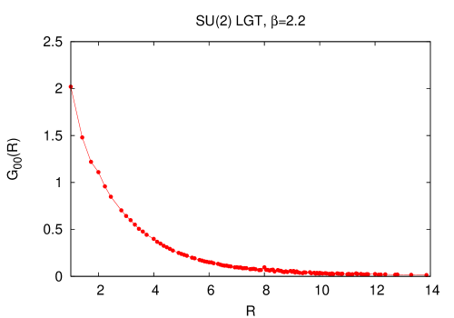
Figure 5: Monte Carlo data for the $00$ component of the equal-times gluon propagator, with $A_{0}^{a}$ extracted from the timelike link variable as described in the text. There is no evidence of a confining Coulomb potential. The simulation is carried out on a $16^{4}$ lattice in SU(2) lattice gauge theory at $\beta=2.2$.

References

- (1) D. Zwanziger, Phys. Rev. Lett. 90, 102001 (2003) [arXiv:hep-lat/0209105].
-
(2)
A. P. Szczepaniak and P. Krupinski,
Phys. Rev. D 73, 116002 (2006)
[arXiv:hep-ph/0604098];
A. P. Szczepaniak and E. S. Swanson, Phys. Lett. B 577, 61 (2003) [arXiv:hep-ph/0308268].;
A. P. Szczepaniak and E. S. Swanson, Phys. Rev. D 65, 025012 (2002) [arXiv:hep-ph/0107078]. - (3) J. Greensite and C. B. Thorn, JHEP 0202, 014 (2002) [arXiv:hep-ph/0112326].
- (4) J. Greensite and Š. Olejník, arXiv:0901.0199 [hep-lat].
- (5) J. Greensite, Š. Olejník, and D. Zwanziger, JHEP 0505, 070 (2005) [arXiv:hep-lat/0407032].
- (6) J. Greensite, Š. Olejník and D. Zwanziger, Phys. Rev. D 69, 074506 (2004) [arXiv:hep-lat/0401003].
- (7) E. Marinari, M. L. Paciello, G. Parisi and B. Taglienti, Phys. Lett. B 298, 400 (1993) [arXiv:hep-lat/9210021].
-
(8)
D. Zwanziger,
Nucl. Phys. B 518, 237 (1998);
V. Gribov, Nucl. Phys. B 139, 1 (1978) -
(9)
A. Cucchieri and D. Zwanziger,
Nucl. Phys. Proc. Suppl. 119, 727 (2003)
[arXiv:hep-lat/0209068];
K. Langfeld and L. Moyaerts, Phys. Rev. D 70, 074507 (2004) [arXiv:hep-lat/0406024];
A. Voigt, E. M. Ilgenfritz, M. Muller-Preussker and A. Sternbeck, Phys. Rev. D 78, 014501 (2008) [arXiv:0803.2307 [hep-lat]]. - (10) J. Greensite and Š. Olejník, Phys. Rev. D 67, 094503 (2003) [arXiv:hep-lat/0302018].
-
(11)
Y. Nakagawa, A. Nakamura, T. Saito, H. Toki and D. Zwanziger,
Phys. Rev. D 73, 094504 (2006)
[arXiv:hep-lat/0603010];
A. Nakamura and T. Saito, Prog. Theor. Phys. 115, 189 (2006) [arXiv:hep-lat/0512042]. - (12) J. E. Mandula and M. Ogilvie, Phys. Lett. B 185, 127 (1987).
- (13) A. Cucchieri and D. Zwanziger, Phys. Rev. D 65, 014002 (2002) [arXiv:hep-th/0008248].
- (14) A. Maas, Eur. Phys. J. C 48, 179 (2006) [arXiv:hep-th/0511307].
- (15) B. Holdom, arXiv:0901.0497 [hep-ph].