The standard model of spin injection

1 Introduction

The generation of nonequilibrium electron spin, as well as the nonequilibrium spin itself, in electronic materials (metals and semiconductors), is called spin accumulation. The most important techniques for spin accumulation are electrical spin injection, optical spin orientation, and spin resonance. By electrical spin injection, or simply spin injection, we mean spin accumulation by injecting spin-polarized electrons from one material to another, by electric current. The source material could be a ferromagnetic metal, for example Fe, in which there is a difference in the densities of spin up and spin down electrons. Such a difference is characterized by a spin polarization. In the ferromagnet the spin polarization exists in equilibrium. In contrast, if electrons from the ferromagnet are injected into a nominally nonmagnetic metal, say, Al, the resulting spin polarization in Al is a nonequilibrium one: spin accumulates in Al. Another possibility is an electrical spin injection between two nonmagnetic materials, say Al and Cu. If one of the materials has a nonequilibrium spin, electric current can lead to spin accumulation in the other material. Electrical spin injection is the main topic of these lecture notes.

The two other techniques for spin accumulation historically preceded spin injection. Optical orientation is a process of generating nonequilibrium spin optically, by exposing the material to a circularly polarized light. The angular momentum of the photons is transferred to the electron spin. Optical orientation is most effective in direct band semiconductors such as GaAs. The historically first technique for investigation nonequilibrium spin has been electron spin resonance. Application of a magnetic field splits the spin up and spin down electron states (Zeeman splitting) with a corresponding equilibrium spin polarization. A microwave radiation can induce transitions between the spin-split states, generating nonequilibrium spin. The spin resonance technique has been used in metals and semiconductors. There are other ways to generate spin accumulation, typically much less efficient as with the three ways mentioned above. One example is the spin Hall effect, in which electric current leads to a separation of spin up and spin down electrons at the edges parallel to the current flow. Another possibility is to first accumulate nuclear spin in the lattice ions; electron spins can be then polarized via the hyperfine interaction.

The standard model of spin injection originates from the proposal of Aronov [1] who suggested the possibility of electrical spin injection from a ferromagnetic to a nonmagnetic conductor. The thermodynamics of spin injection has been developed by Johnson and Silsbee, who also formulated a drift-diffusion transport model for spin transport across ferromagnet/nonmagnet (F/N) interfaces [2, 3]. This model has been shown to be essentially equivalent to the standard model as presented here [4, 5]. The theory of spin injection was further developed in [6, 7, 8, 9, 10, 11, 12, 13, 14, 15, 16, 17, 18, 19, 20]. In particular the presentation of Rashba [14, 15] has inspired the formulation of the standard model of spin injection in the reviews [4, 5] which these lecture notes follow and extend. These reviews should be consulted for original references and examples of experimental results.

2 Simple model of spin injection

Perhaps the simplest model of spin injection considers a steady flow of a spin-polarized electric current from a ferromagnet to a nonmagnetic conductor. The ferromagnet has an electron spin polarization $P_{0}$; for the present purposes $P_{0}$ is the relative difference between the “relevant” densities of spin up and spin down electrons. More specific definitions of the term are given later. In a typical ferromagnetic metal $P_{0}$ is 10–50%. In nonmagnetic metals the spin polarization at equilibrium vanishes.

Calling the ferromagnetic conductor $F$ and the nonmagnetic conductor $N$, we have a simple F/N junction. We wish to answer the following question:

Given the equilibrium spin polarization $P_{0}$ in the ferromagnet, what is the spin accumulation in the nonmagnetic conductor if electric current $j$ flows through the junction?

In order to answer this question, we need to know how much spin per unit time arrives from $F$ to $N$. The simplest answer would be $j_{s0}/(-e)$, where the spin current

$$j_{s0}=P_{0}j,$$ (1)

as the spins are attached to the electrons flowing through the interface. We can take this value as a very rough estimate of what to expect. What Eq. 1 neglects is the possibility of spin accumulation in the ferromagnet. As we will see later, spin indeed accumulates in the ferromagnet, strongly modifying the above estimate for $j_{s0}$. Another simplification we made is to suppose that the spin is preserved during crossing the interface. This approximation is actually quite good and will be used in the standard model as well.

Knowing the spin current at the interface, we can focus on the $N$ region. What happens to the spin which crosses the interface? Unlike charge, spin is not conserved. Spin relaxes to the equilibrium value (which is zero in $N$) due to spin-flip scattering and other spin-randomizing processes. As a result, the motion of the spin in the presence of spin current will be diffusive. For the spin density $s(x)$ in the $N$ region we can then write a diffusion equation

$$\frac{d^{2}s}{dx^{2}}=\frac{s}{L_{s}^{2}},$$ (2)

where $L_{s}$ is the spin diffusion length in the nonmagnetic conductor. In terms of diffusivity $D$ and the spin relaxation time $\tau_{s}$ the spin diffusion length is given as

$$L_{s}=\sqrt{D\tau_{s}}.$$ (3)

The diffusion equation has a general solution,

$$s(x)=s_{0}e^{-x/L_{s}},$$ (4)

where $s_{0}=s(0)$ is the spin density at the interface, $x=0$. Above we applied the physical condition that $s(\infty)=0$.

What remains is to connect the spin density $s_{0}$ with the spin current $j_{s0}$. Since the transport of spin is diffusive, the spin current is

$$j_{s}=(-e)\times-D\frac{ds}{dx}.$$ (5)

Note that we define the spin current as the electric current corresponding to the spin flow—that is why the multiplication by $-e$ above. At $x=0$, using Eq. 4, we obtain

$$j_{s}=\frac{-eD}{L_{s}}s_{0}e^{-x/L_{s}}.$$ (6)

Assuming that the spin current is continuous across the interface (spin relaxation is absent there), $j_{s}(0)=j_{s0}$, we find

$$s_{0}=j_{s0}\frac{L_{s}}{-eD}.$$ (7)

The full spin density profile in $N$ is given by

$$s(x)=j_{s0}\frac{L_{s}}{-eD}e^{-x/L_{s}}.$$ (8)

The total amount of accumulated spin is

$$s_{\rm acc}=\int_{0}^{\infty}s(x)dx=\frac{j_{s_{0}}L_{s}^{2}}{-eD}=\frac{j_{s0}}{-e}\tau_{s}.$$ (9)

In effect, the spin is pumped into the $N$ region. The steady state is achieved by spin relaxation: The more pumping and the less spin relaxation, the higher is the spin accumulation.

3 Spin-polarized transport: concepts and definitions

Quasichemical potentials.

In thermodynamic equilibrium the chemical potential $\eta$ throughout the electronic system is uniform, determining the electron density

$$n_{0}(\eta)=\int d\epsilon g(\epsilon)f_{0}(\epsilon),$$ (10)

where $g(\epsilon)$ is the electronic density of states at the energy $\epsilon$ and $f_{0}$ is the equilibrium Fermi-Dirac distribution function at a given temperature $T$,

$$f_{0}(\epsilon)=\frac{1}{\exp(\epsilon-\eta)/k_{B}T+1}.$$ (11)

In the presence of an electrostatic potential $\phi(x)$ giving rise to electric current due to the electric field $E=-\nabla\phi$ inside the conductor, the chemical potential is no longer uniform (the system is no longer an equilibrium one):

$$\eta\to\eta+e\mu(x),$$ (12)

where the space dependent addition $\mu(x)$ is the quasichemical potential. Since typically the momentum relaxes on length scales smaller than the variation of $\phi$, we can assume the local nonequilibrium electron distribution function to be only energy dependent,

$$f(\epsilon,x)=f_{0}[\epsilon-e\phi(x)-\eta-e\mu(x)].$$ (13)

Then the nonequilibrium electron density is

$$n(x)=\int d\epsilon g(\epsilon)f(\epsilon,x)=n_{0}(\eta+e\mu+e\phi).$$ (14)

Local charge neutrality.

We make the assumption that charge does not accumulate inside the conductor under bias $\phi$. This is an excellent approximation for metals and highly doped (degenerate) semiconductors. On the other hand, charge can be injected and accumulated in nondegenerate semiconductors due to the large screening length. For such cases the standard spin injection model does not apply. The local charge neutrality means that

$$n(x)=n_{0}.$$ (15)

This gives the general condition,

$$\mu(x)=-\phi(x).$$ (16)

The quasichemical potential fully balances the electrostatic potential.

Electric current.

The electric current comprises the drift current, proportional to the electric field $E=-\nabla\phi$, and the diffusion current, proportional to the gradient of the electron density $\nabla n$:

$$j=\sigma E+eD\nabla n.$$ (17)

The two proportionality parameters are conductivity $\sigma$ and diffusivity, $D$. Due to charge neutrality the diffusion current is absent. We will keep it in the discussion as diffusion will be present in the spin flow. Using Eq. 14, we write

$$\nabla n=\frac{\partial n_{0}}{\partial\eta}e\nabla\phi+\frac{\partial n_{0}}{\partial\eta}e\nabla\mu.$$ (18)

Substituting to Eq. 17 gives

$$j=\left(-\sigma+e^{2}D\frac{\partial n_{0}}{\partial\eta}\right)\nabla\phi+e^{2}D\frac{\partial n_{0}}{\partial\eta}\nabla\mu.$$ (19)

There are two important consequences of this equation. First, if the chemical potential is uniform, $\nabla\mu=0$, the current has to vanish. This gives the condition on the conductivity,

$${\sigma=e^{2}D\frac{\partial n_{0}}{\partial\eta},}$$ (20)

known as the Einstein relation. To a good approximation $\partial n_{0}/\partial\eta=g(\eta)$, where $g(\eta)$ is the electron density of states at the Fermi level. Second, using the Einstein relation, the electric current is expressed through the quasichemical potential only,

$${j=\sigma\nabla\mu.}$$ (21)

This equation generalizes the familiar $j=\sigma E$ to situations with diffusive currents. The gradient of $\mu$ carries information on both drift and diffusion.

In a steady state, the continuity of the electric current requires that

$$\nabla j=0,$$ (22)

that is, the current is uniform. We can also identify the total increase of the quasichemical potential across the system with applied voltage. Indeed, for a uniform system of length $L$ integration of Eq. 21 gives

$$\Delta\mu=\frac{L}{\sigma}j={\cal R}j,$$ (23)

where $\cal{R}$ is the electric resistance of the system.

Contact resistance.

At sharp contacts the chemical potential need not be continuous. Instead of Eq. 21 we write

$${j=\Sigma\Delta\mu,}$$ (24)

in which $\Sigma$ is the contact conductance and $\Delta\mu$ is the increase of the chemical potential across the interface. The contact electrical resistance is

$${\cal R}_{c}=\frac{1}{\Sigma_{c}}.$$ (25)

Problem. Consider two conductors, A and B, forming a junction with contact resistance ${\cal R}_{c}$. The conductivities of A and B are $\sigma_{A}$ and $\sigma_{B}$. Integrate Eq. 21 for each conductor, and apply the condition of the electric current continuity together with Eq. 24 to obtain $j$ as a function of the applied voltage. What is the total junction resistance? The standard model of spin injection goes in the same spirit as this exercise.

Spin density and spin polarization.

Consider a conductor with the electron density $n$. This density comprises the densities of spin up and spin down electrons:

$$n=n_{\uparrow}+n_{\downarrow}.$$ (26)

We define the spin density as

$$s=s_{\uparrow}-s_{\downarrow}.$$ (27)

A relative difference between the spin up and spin down densities is the spin polarization of the density,

$$P_{n}=\frac{s}{n}.$$ (28)

We add the label $n$ to stress that we speak about the density spin polarization. For a general spin-resolved quantity $X$, we will have

$$P_{X}=\frac{X_{\uparrow}-X_{\downarrow}}{X_{\uparrow}+X_{\downarrow}},$$ (29)

and call it the “spin polarization of X.”

Spin accumulation.

Let us allow for different densities of states $g_{\uparrow}$ and $g_{\downarrow}$ at the Fermi level, as well as different quasichemical potentials $\mu_{\uparrow}$ and $\mu_{\downarrow}$ for spin up and spin down electrons. The equilibrium chemical potential $\eta$ is the same for both spin species. Then

$$n_{\uparrow}(x) = n_{\uparrow 0}\left(\eta+e\mu_{\uparrow}+e\phi\right)\approx n_{\uparrow 0}+\frac{\partial n_{\uparrow 0}}{\partial\eta}\left(e\mu_{\uparrow}+e\phi\right),$$ (30)

$$n_{\downarrow}(x) = n_{\downarrow 0}\left(\eta+e\mu_{\downarrow}+e\phi\right)\approx n_{\downarrow 0}+\frac{\partial n_{\downarrow 0}}{\partial\eta}\left(e\mu_{\downarrow}+e\phi\right),$$ (31)

where we have expanded the nonequilibrium densities assuming that $\mu+\phi$ is much smaller than the equilibrium chemical potential $\eta$; this is a good approximation as it is the electrons close to the Fermi level that contribute to spin accumulation in degenerate conductors. Since $\partial n_{0}/\partial\eta=g$, we find

$$n_{\uparrow}(x) = n_{\uparrow 0}+g_{\uparrow}e\mu_{\uparrow}+g_{\uparrow}e\phi,$$ (32)

$$n_{\downarrow}(x) = n_{\downarrow 0}+g_{\downarrow}e\mu_{\downarrow}+g_{\downarrow}e\phi.$$ (33)

The local charge neutrality, $n_{\uparrow}+n_{\downarrow}=n_{0}$, then leads to the condition,

$$g(\mu+\phi)+g_{s}\mu_{s}=0,$$ (34)

where

$$g = g_{\uparrow}+g_{\downarrow}$$ (35)

$$g_{s} = g_{\uparrow}-g_{\downarrow}.$$ (36)

For nonmagnetic conductors $g_{s}=0$, recovering Eq. 16. From Eqs. 32 and 33, using the charge neutrality Eq. 34, we obtain for the spin density

$$s=s_{0}+eg_{s}(\mu+\phi)+eg\mu_{s}=s_{0}+4e\mu_{s}\frac{g_{\uparrow}g_{\downarrow}}{g}.$$ (37)

Here we denoted the quasichemical and spin quasichemical potentials

$$\mu = (\mu_{\uparrow}+\mu_{\downarrow})/2,$$ (38)

$$\mu_{s} = (\mu_{\uparrow}-\mu_{\downarrow})/2.$$ (39)

The accumulated nonequilibrium spin $\delta s$ defined by

$$s=s_{0}+\delta s,$$ (40)

is then

$$\delta s=4e\frac{g_{\uparrow}g_{\downarrow}}{g}\mu_{s}.$$ (41)

Both the nonequilibrium spin density $\delta s$ and the spin quasichemical potential $\mu_{s}$ are often termed spin accumulation.

Charge and spin currents.

Charge current is the total electric current carried by spin up and spin down electrons,

$$j=j_{\uparrow}+j_{\downarrow}.$$ (42)

By contrast, spin current is the difference between the electric currents carried by spin up and spin down electrons:

$$j_{s}=j_{\uparrow}-j_{\downarrow}.$$ (43)

The two spin components of the electric current are given by

$$j_{\uparrow} = \sigma_{\uparrow}\nabla\mu_{\uparrow},$$ (44)

$$j_{\downarrow} = \sigma_{\downarrow}\nabla\mu_{\downarrow}.$$ (45)

We have labeled the conductivities and the quasichemical potentials with the corresponding spin index. In nonmagnetic conductors $\sigma_{\uparrow}=\sigma_{\downarrow}$. Let us introduce the charge and spin conductivities as follow:

$$\sigma = \sigma_{\uparrow}+\sigma_{\downarrow},$$ (46)

$$\sigma_{s} = \sigma_{\uparrow}-\sigma_{\downarrow}.$$ (47)

The electric charge and spin currents become

$$j = \sigma\nabla\mu+\sigma_{s}\nabla\mu_{s},$$ (48)

$$j_{s} = \sigma_{s}\nabla\mu+\sigma\nabla\mu_{s}.$$ (49)

For a nonmagnetic conductor $\sigma_{s}=0$ and the charge and spin currents decouple; the charge current is driven by the gradient of the quasichemical potential while the spin current is driven by the gradient of the spin accumulation. In a ferromagnetic conductor $\sigma_{s}\neq 0$ and a gradient in spin accumulation can cause a charge current. Similarly, a gradient in the quasichemical potential alone would cause a spin current.

Current spin polarization.

The spin polarization of the electric current $P_{j}$ is defined according to Eq. 29,

$$P_{j}=\frac{j_{\uparrow}-j_{\downarrow}}{j_{\uparrow}+j_{\downarrow}}=\frac{j_{s}}{j}.$$ (50)

Extract $\nabla\mu$ from Eq. 48,

$$\nabla\mu=\frac{1}{\sigma}\left(j-\sigma_{s}\nabla\mu_{s}\right),$$ (51)

and substitute into Eq. 49:

$$j_{s}=\sigma_{s}\nabla\mu+\sigma\nabla\mu_{s}=P_{\sigma}j+4\frac{\sigma_{\uparrow}\sigma_{\downarrow}}{\sigma}\nabla\mu_{s}.$$ (52)

Here $P_{\sigma}$ is the conductivity spin polarization,

$$P_{\sigma}=\frac{\sigma_{\uparrow}-\sigma_{\downarrow}}{\sigma_{\uparrow}+\sigma_{\downarrow}}=\frac{\sigma_{s}}{\sigma}.$$ (53)

The spin and charge currents are coupled through $P_{\sigma}$. Finally, the current spin polarization is

$${P_{j}=\frac{j_{s}}{j}=P_{\sigma}+\frac{1}{j}4\nabla\mu_{s}\frac{\sigma_{\uparrow}\sigma_{\downarrow}}{\sigma}}.$$ (54)

In nonmagnetic conductors $P_{\sigma}=0$ and spin current is due to the gradient in spin accumulation only.

Spin-polarized currents in contacts.

The above formalism can be rewritten for contacts with discrete jumps of the quasichemical potentials. Following Eq. 24, the spin-resolved currents are

$$j_{\uparrow} = \Sigma_{\uparrow}\Delta\mu_{\uparrow},$$ (55)

$$j_{\downarrow} = \Sigma_{\downarrow}\Delta\mu_{\downarrow}.$$ (56)

Defining the contact charge and spin conductances as

$$\Sigma = \Sigma_{\uparrow}+\Sigma_{\downarrow},$$ (57)

$$\Sigma_{s} = \Sigma_{\uparrow}-\Sigma_{\downarrow},$$ (58)

we can write

$$j = \Sigma\Delta\mu+\Sigma_{s}\Delta\mu_{s},$$ (59)

$$j_{s} = \Sigma_{s}\Delta\mu+\Sigma\Delta\mu_{s}.$$ (60)

Going through similar steps as above of Eq. 54, we obtain for the spin current polarization in the contact

$${P_{jc}=P_{\Sigma}+\frac{1}{j}\frac{\Delta\mu_{s}(0)}{R_{c}}.}$$ (61)

Here

$$P_{\Sigma}=\frac{\Sigma_{\uparrow}-\Sigma_{\downarrow}}{\Sigma_{\uparrow}+\Sigma_{\downarrow}}=\frac{\Sigma_{s}}{\Sigma},$$ (62)

is the contact spin conductance polarization and

$$R_{c}=\frac{\Sigma}{4\Sigma_{\uparrow}\Sigma_{\downarrow}},$$ (63)

is the effective contact resistance, determining the drop of the spin accumulation across the contact; $R_{c}$ is a quarter of the series resistance of the spin up and spin down contact resistances. In a spin unpolarized contact $R_{c}={\cal R}_{c}=1/\Sigma$.

Diffusion of spin accumulation.

In nonmagnetic systems it is sufficient to use the continuity of the charge current, Eq. 22, to find the profile of the quasichemical potential $\mu(x)$. In the presence of spin polarization, we need a continuity condition for the spin current as well; the continuity of the charge current remains unchanged: $\nabla j=0$. Since, unlike charge, spin is not conserved, the continuity equation for the spin current is

$$\nabla j_{s}=e\frac{\delta s}{\tau_{s}},$$ (64)

where $\delta s$ is the deviation of the spin density from its equilibrium value: $s=s_{\rm eq}+\delta s$. The divergence of the spin current is proportional to the rate of spin relaxation $1/\tau_{s}$, with $\tau_{s}$ denoting the spin relaxation time. On one hand,

$$\nabla j_{s}=e\frac{\delta s}{\tau_{s}}=4e^{2}\mu_{s}\frac{g_{\uparrow},g_{\downarrow}}{g}\frac{1}{\tau_{s}}$$ (65)

where we used Eq. 41 for $\delta s$. On the other hand, Eq. 52 gives

$$\nabla j_{s}=\nabla\left(P_{\sigma}j+\nabla\mu_{s}\frac{4\sigma_{\uparrow}\sigma_{\downarrow}}{\sigma}\right)=4\frac{\sigma_{\uparrow}\sigma_{\downarrow}}{\sigma}\nabla^{2}\mu_{s}.$$ (66)

Comparing the two we get the following diffusion equation for spin accumulation:

$${\nabla^{2}\mu_{s}=\frac{\mu_{s}}{L_{s}^{2}},}$$ (67)

where the generalized spin diffusion length $L_{s}$ is

$$L_{s}=\sqrt{\overline{D}\tau_{s}},$$ (68)

and the generalized diffusivity

$$\overline{D}=\frac{g}{g_{\uparrow}/D_{\downarrow}+g_{\downarrow}/D_{\uparrow}}.$$ (69)

In a nonmagnetic conductor $\overline{D}=D$. Representative spin relaxation times $\tau_{s}$ in nonmagnetic metals and semiconductors are nanoseconds, and spin diffusion lengths micrometers. In ferromagnetic conductors these quantities are smaller by several orders of magnitude.

Spin-charge coupling.

Let us write Eq. 51 as

$$\nabla\mu=\frac{j}{\sigma}-P_{\sigma}\nabla\mu_{s},$$ (70)

and integrate it over a homogeneous region of a conductor:

$$\Delta\mu=j{\cal R}-P_{\sigma}\Delta\mu_{s},$$ (71)

where $\cal R$ is the electrical resistances of the region. Consider a homogeneous ferromagnetic conductor of length $L\gg L_{s}$, stretching from $x=-L$ to $x=0$. Assume that at $x=0$ there is a spin accumulation $\mu_{s}(0)$. Applying the above equation gives

$$\mu(0)-\mu(-L)=j{\cal R}-P_{\sigma}\mu_{s}(0),$$ (72)

where the conductor’s electric resistance is ${\cal R}=L/\sigma$ and we assumed absence of spin accumulation at $x=-L$. In a nonmagnetic conductor $P_{\sigma}=0$ and the increase of the quasichemical potential is due to the charge current flow only. In a ferromagnetic conductor the increase is also due to the spin accumulation. In an open circuit ($j=0$) the increase in the quasichemical potential is

$$\mu(0)-\mu(-L)=-P_{\sigma}\mu_{s}(0),$$ (73)

This increase defines the electromotive force (emf) per unit charge generated by the spin accumulation in the ferromagnetic conductor. Similarly, we can calculate the corresponding drop in the electric potential,

$$\phi(-L)-\phi(0)=(P_{g}-P_{\sigma})\mu_{s}(0),$$ (74)

where we used the local neutrality condition, Eq. 34. The density of states spin polarization is

$$P_{g}=\frac{g_{\uparrow}-g_{\downarrow}}{g_{\uparrow}+g_{\downarrow}}=\frac{g_{s}}{g}.$$ (75)

Equation 74 is an example of spin-charge coupling: The presence of a spin accumulation in a conductor with an equilibrium spin polarization, a nonequilibrium voltage drop (electromotive force) develops. Electrostatic detection of the voltage drop then allows to extract the magnitude of the spin accumulation.

4 The standard model of spin injection: $F$/$N$ junction

We pose the following question:

Knowing the equilibrium materials parameters of a ferromagnet ($F$), a nonmagnetic conductor ($N$), as well as the properties of the contact ($C$) between them, what is the spin current polarization and spin accumulation in $N$, in the presence of electric current $j$?

The scheme of the $F$/$N$ junction we consider is in Fig. 1. The spin current polarization at the contact is termed spin injection efficiency. We denote it as $P_{j}$. To obtain $P_{j}$ we need to consider spin-polarized transport separately in the three regions: $F$, $C$, and $N$. The solutions for the transport equations will then be connected by suitable continuity conditions. We also add labels $F$, $C$, and $N$ to the quantities pertaining to the three regions.

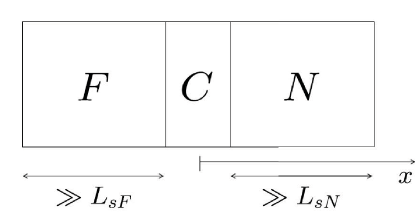
Figure 1: The $F$/$N$ junction above comprises a ferromagnetic conductor $F$, a nonmagnetic conductor $N$, as well as the contact $C$ between them at $x=0$. It is assumed that the widths of the $F$ and $N$ regions are much larger (we call their size “$\infty$”) than the corresponding spin diffusion length.

Ferromagnetic conductor.

The ferromagnetic conductor occupies the region $(-\infty,0)$. The spin accumulation profile is given by the solution of the diffusion equation, Eq. 67, as

$$\mu_{sF}=\mu_{sF}(0)e^{x/L_{sF}}.$$ (76)

We have applied the condition that there is no spin accumulation at $x=-\infty$: $\mu_{sF}(-\infty)=0$. This condition is well satisfied if the length of the ferromagnet, indicated by “$\infty$”, is much larger than the spin diffusion length $L_{sF}$. From the above we have

$$\nabla\mu_{sF}(0)=\frac{\mu_{sF}(0)}{L_{sF}}.$$ (77)

Substituting to Eq. 54 we obtain the spin current polarization in the $F$ region of the contact

$$P_{jF}(0)=P_{\sigma F}+\frac{1}{j}\frac{\mu_{sF}(0)}{R_{F}},$$ (78)

where we denote

$$R_{F}=\frac{\sigma_{F}}{4\sigma_{F\uparrow}\sigma_{F\downarrow}}L_{sF},$$ (79)

the effective resistance of the ferromagnet; $R_{F}$ is a quarter of the serial resistance of the spin up and spin down resistances of a piece of the ferromagnet of length $L_{sF}$. We stress that $R_{F}$ is not the actual resistance of the $F$ region ${\cal R}_{F}$, which is

$${\cal R}_{F}=\frac{``\infty"}{\sigma_{\uparrow}+\sigma_{\downarrow}},$$ (80)

given as a parallel resistance of the two spin channels over the entire size $``\infty"$ of the ferromagnet. The two resistances, $R_{F}$ and ${\cal R}_{F}$ can be very different!

Nonmagnetic conductor.

In a nonmagnetic conductor the transport and materials parameters are spin independent and all the equilibrium polarizations, such as $P_{\sigma}$ or $P_{g}$, vanish. The profile of the spin accumulation is

$$\mu_{sN}=\mu_{sN}(0)e^{-x/L_{sF}},$$ (81)

satisfying the boundary condition $\mu_{sN}(\infty)=0$. We then have

$$\nabla\mu_{sN}(0)=-\frac{\mu_{sN}(0)}{L_{sN}},$$ (82)

and the spin current polarization at the contact

$$P_{jN}(0)=-\frac{1}{j}\frac{\mu_{sN}(0)}{R_{N}},$$ (83)

where

$$R_{N}=\frac{L_{sN}}{\sigma_{N}},$$ (84)

is the effective resistance of the $N$ region; $R_{N}$ is the resistance of a piece of a conductor of size $L_{sN}$. Again, $R_{N}$ can be very different from the actual electric resistance of the $N$ region, ${\cal R}_{N}$.

Contact region.

The contact region is described by Eq. 61. For our $F$/$N$ contact the spin current polarization is

$$P_{jc}=P_{\Sigma}+\frac{1}{j}\frac{\mu_{sN}(0)-\mu_{sF}(0)}{R_{c}}.$$ (85)

Spin injection efficiency.

We have three equations for the spin current polarizations, Eqs. 78, 83, 85, in three different regions. We assume that spin is conserved across the contact. As a consequence, the spin current (and thus spin current polarization) is continuous there:

$$P_{j}\equiv P_{jF}(0)=P_{jN}(0)=P_{jc}.$$ (86)

Solving this straightforward algebraic problem leads to the important expression for the spin injection efficiency:

$${P_{j}=\frac{R_{F}P_{\sigma F}+R_{c}P_{\Sigma}}{R_{F}+R_{c}+R_{N}}=\langle P_{\sigma}\rangle_{R}.}$$ (87)

This equation is one of the main results of the standard model of spin injection. The spin injection efficiency is the weighted average of the equilibrium spin conductance polarizations of the system; the weight is the relative effective resistance.

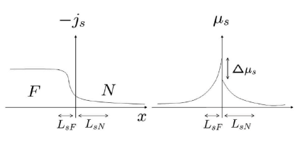
Figure 2: Sketch of the spatial profile of the spin current $j_{s}$ and the spin quasichemical potential $\mu_{s}$ in an $F$/$N$ junction in the spin injection regime. While the spin current is continuous throughout the junction, the spin quasichemical potential experiences a jump at the contact.

Problem. $F$/$F$ junction. Calculate the spin injection efficiency for a $F$/$F$ junction of two different ferromagnets. Show that $P_{j}=\langle P_{\sigma}\rangle_{R}$ still holds.

Spin injection and spin extraction.

Knowing $P_{j}$ we can calculate the spin accumulation in the $N$ region,

$$\mu_{sN}(0)=-jP_{j}R_{N},$$ (88)

and the corresponding spin density polarization,

$$P_{n}(0)=\frac{s(0)}{n}=e\mu_{sN}(0)\frac{g_{N}}{n}=-jeR_{N}\frac{g_{N}}{n}P_{j}.$$ (89)

Since the spin polarization is proportional to the electric current, the electric spin injection is a realization of spin pumping. In a typical spin injection experiment electrons flow from $F$ to $N$, so that $j<0$. In this case $P_{n}(0)$ has the same size as $P_{j}$ and we speak of spin injection. If the electric current is reversed, $j<0$, electrons from $N$ flow into $F$. Now $P_{n}(0)$ has the opposite sign to $P_{j}$ and we speak of spin extraction. For a positive $P_{j}$, for example, more spin up than spin down electrons are transported through the contact, leaving a negative spin density in the $N$ region. A sketch of the profile of the spin current and spin quasichemical potential across an $F$/$N$ junction is shown in Fig. 2.

Equivalent circuit.

The standard model of spin injection can be formulated by a simple equivalent circuit model, shown in Fig. 3. The model is a parallel circuit with spin up and spin down channels. Each region is characterized by the corresponding effective resistance.

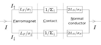
Figure 3: Equivalent circuit of a $F$/$N$ junction in the spin injection regime. The electric current splits into spin up and spin down channels, each with a series of three effective resistances as indicated.

Problem. Calculate $I_{s}=I_{\uparrow}-I_{\downarrow}$ from the equivalent circuit model and show that $P_{j}=I_{s}/I$ agrees with Eq. 87.

Problem. Formulate the equivalent circuit model for a F/F junction.

Problem. $F$/$N$/$N$ junction. Consider electrical spin injection in an $F$/$N$/$N$ junction in which the two $N$ regions are different (say, GaAs and Si). Calculate the spin injection efficiency at the $N$/$N$ interface. What is the spin accumulation at both sides of this interface? Sketch the profile of the spin accumulation across this junction.

5 Nonequilibrium resistance and spin bottleneck

In the absence of spin accumulation the resistance of the F/N junction is ${\cal R}_{F}+{\cal R}_{N}+{\cal R}_{c}$. Spin accumulation leads to an additional positive resistance $\delta{\cal R}$ so that the increase of the quasichemical potential (which generates the emf) is

$$\mu_{N}(\infty)-\mu_{F}(-\infty)=({\cal R}_{F}+{\cal R}_{N}+{\cal R}_{c}+\delta{\cal R})j.$$ (90)

Let us apply Eq. 71 to the three regions, $F$, $C$, and $N$, successively:

$$\mu_{F}(0)-\mu_{F}(-\infty) = j{\cal R}_{F}-P_{\sigma F}\mu_{sF}(0),$$ (91)

$$\mu_{N}(0)-\mu_{F}(0) = j{\cal R}_{c}-P_{\Sigma}\left[\mu_{sN}(0)-\mu_{sF}(0)\right],$$ (92)

$$\mu_{N}(\infty)-\mu_{N}(0) = j{\cal R}_{N}.$$ (93)

We have used that $\mu_{sF}(-\infty)=0$. Summing up the above equations gives for the nonequilibrium resistance

$$\delta{\cal R}=-(P_{\sigma F}-P_{\Sigma})\mu_{sF}(0)-P_{\Sigma}\mu_{sN}(0).$$ (94)

Expressing the spin quasichemical potentials at $x=0$ in terms of the spin injection efficiency, see Eqs. 78 and 83,

$$\mu_{sF}(0) = jR_{F}(P_{j}-P_{\sigma F}),$$ (95)

$$\mu_{sN}(0) = -jR_{N}P_{j},$$ (96)

we get

$$\delta{\cal R}=-P_{\Sigma}(P_{j}-P_{\Sigma})R_{c}-P_{\sigma F}(P_{j}-P_{\sigma F})R_{F}.$$ (97)

Using the expression for $P_{j}$ in Eq. 87, we obtain the final result

$$\delta{\cal R}=\frac{R_{N}(P_{\Sigma}^{2}R_{c}+P_{\sigma F}^{2}R_{F})+R_{F}R_{c}(P_{\sigma F}-P_{\Sigma})^{2}}{R_{F}+R_{c}+R_{N}}>0.$$ (98)

The nonequilibrium resistance is always positive!

Problem. Obtain the nonequilibrium resistance $\delta{\cal R}$ from the equivalent circuit model in Fig. 3, as $\delta{\cal R}={\cal R}-L_{sF}/\sigma_{F}-L_{sN}/\sigma_{N}$.

What is the reason behind the additional positive resistance due to spin accumulation? As the nonequilibrium spin piles up in the ferromagnet and the spin-polarizing contact region, the spin diffusion there pushes the electrons against the flow of the electric current. Indeed, the electric current brings electrons from the spin-polarized region to the nonmagnetic conductor, while the spin diffusion in the ferromagnet and the contact drives them back to the ferromagnet. This spin bottleneck effect causes the additional electrical resistance of the junction.

6 Transparent and tunnel contacts, conductivity mismatch

Two important cases are analyzed: transparent and tunnel contacts.

Transparent contacts.

By transparent contacts we mean the condition

$$R_{c}\ll R_{N},R_{F}.$$ (99)

This is the case of usual ohmic contacts between two metals or degenerate semiconductors. Using our results for the $F$/$N$ junction, a transparent contact is characterized by the spin efficiency

$$P_{j}=\frac{R_{F}}{R_{F}+R_{N}}P_{\sigma F}.$$ (100)

For metals $\sigma_{F}$ is usually somewhat less than $\sigma_{N}$, as $L_{sN}\gg L_{sF}$. We then get

$$P_{j}\approx(\sigma_{N}/\sigma_{F})(L_{sF}/L_{sN}).$$ (101)

If $N$ is a semiconductor while $F$ is a metal, so that $\sigma_{N}\ll\sigma_{F}$, the spin injection efficiency is greatly reduced. This inefficiency of the spin injection from a ferromagnetic metal to a nonmagnetic semiconductor via a transparent contact is known as the conductivity mismatch problem, since it comes from the greatly different conductivities of the two regions of the junctions.

The nonequilibrium resistance of a transparent contact is

$$\delta{\cal R}=\frac{R_{N}R_{F}}{R_{N}+R_{F}}P_{\sigma F}^{2}.$$ (102)

Again, since typically $R_{N}$ is greater than $R_{F}$,

$$\delta{\cal R}\approx R_{F}P_{\sigma F}^{2}=\frac{L_{sF}}{\sigma_{F}}P_{\sigma F}^{2}.$$ (103)

In the extreme limit of the conductivity mismatch, the nonequilibrium resistance will be negligible as compared to the usual electrical junction resistance which will be dominated by ${\cal R}_{N}$.

Tunnel contacts.

By tunnel contacts we mean

$$R_{c}\gg R_{N},R_{F}.$$ (104)

The contact dominates the electric properties of the junction. The spin injection efficiency for a tunnel contact is

$$P_{j}\approx P_{\Sigma}.$$ (105)

The contact also dominates the spin injection efficiency. The conductance mismatch in tunnel contacts plays no role and spin injection from a ferromagnetic metal to a nonmagnetic semiconductor can be highly efficient.

The nonequilibrium resistance of a tunnel contact is

$$\delta{\cal R}=R_{N}P_{\Sigma}^{2}+R_{F}(P_{\sigma F}-P_{\Sigma})^{2}.$$ (106)

This is in general much less than the electric resistance of the contact, ${\cal R}_{c}$.

Problem. Spin accumulation in transparent and tunnel junctions. Calculate the spin accumulation $\mu_{sN}(0)$ and the spin density polarization $P_{\sigma N}(0)$ in a transparent and a tunnel $F$/$N$ junction. What is the spin density polarization in the conductivity mismatch problem? Can it be significant?

Problem. Equivalent circuit of the conductivity mismatch problem. Draw the equivalent circuit for the conductivity mismatch problem of a transparent $F$/$N$ junction and use it to explain the spin injection inefficiency.

7 Silsbee-Johnson spin-charge coupling

Driving electric current through a $F$/$N$ interface generates spin accumulation by the process of spin injection. The Silsbee-Johnson spin charge coupling is the inverse of spin injection: emf develops by the presence of a spin accumulation in the proximity of a ferromagnetic conductor. We will analyze the coupling in an open $F$/$N$ junction, that is in the absence of electric current ($j=0$), under the condition of $\mu_{sN}(\infty)\neq 0$ which models a source of nonequilibrium spin far in the nonmagnetic region. The scheme is shown in Fig. 4.

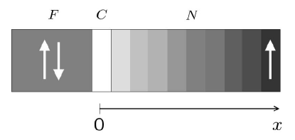
Figure 4: Scheme of the Silsbee-Johnson spin-charge coupling. A spin source at the far right of the $N$ region drives spin by diffusion towards the spin-polarizing contact and ferromagnet. The proximity of the nonequilibrium spin and the equilibrium spin polarization gives rise to an emf in the open circuit (or electric current when the circuit is closed).

The induced emf is the increase of the quasichemical potential across the junction,

$${\rm emf}=\mu_{N}(\infty)-\mu_{F}(-\infty).$$ (107)

The charge neutrality and the physical condition that $\mu_{sF}(-\infty)=0$ guarantee that the emf can be detected as a drop of the electric voltage:

$${\rm emf}=\mu_{N}(\infty)-\mu_{F}(-\infty)=\phi_{F}(-\infty)-\phi_{N}(\infty).$$ (108)

Our strategy is to first express the quasichemical potential increase in terms of the spin accumulations at the contact, and then use the spin current continuity at the contact as well as the diffusion of the spin accumulation to find the spin accumulations.

In the absence of electric current we can apply Eq. 71 to $F$, $C$, and $N$ regions sequentially:

$$\mu_{F}(0)-\mu_{F}(-\infty) = -P_{\sigma_{F}}\mu_{sF}(0),$$ (109)

$$\mu_{N}(0)-\mu_{F}(0) = -P_{\Sigma}\left[\mu_{sN}(0)-\mu_{sF}(0)\right],$$ (110)

$$\mu_{N}(\infty)-\mu_{N}(0) = 0.$$ (111)

In the nonmagnetic conductor there is no voltage drop associated with the presence of spin accumulation if $j=0$. Summing up the above equations gives

$${\rm emf}=\mu_{N}(\infty)-\mu_{F}(-\infty)=\mu_{sF}(0)(P_{\Sigma}-P_{\sigma F})-\mu_{sN}(0)P_{\Sigma}.$$ (112)

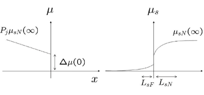
Figure 5: Sketch of the spatial profile of the quasichemical potential $\mu$ (left) and the spin quasichemical potential $\mu_{s}$ (right) in a $F$/$N$ junction in the spin-charge coupling regime.

In the $N$ region, due to the presence of spin accumulation at the far right, the spin accumulation diffusion profile is

$$\mu_{sN}(x)=\mu_{sN}(\infty)+\left[\mu_{sN}(0)-\mu_{sN}(\infty)\right]e^{-x/L_{sN}},$$ (113)

as can be verified by direct substitution to the diffusion equation, Eq. 67. To calculate the spin current at $x=0$ in the $N$ region we need the gradient,

$$\nabla\mu_{sN}(0)=-\frac{1}{L_{sN}}\left[\mu_{sN}(0)-\mu_{sN}(\infty)\right].$$ (114)

We are now ready to calculate the spin currents at the interface, for the three regions. Equation 52 gives

$$j_{sN}(0) = -\frac{1}{R_{N}}\left[\mu_{sN}(0)-\mu_{sN}(\infty)\right],$$ (115)

$$j_{sF}(0) = \frac{1}{R_{F}}\mu_{sF}(0),$$ (116)

$$j_{sc} = \frac{1}{R_{c}}\left[\mu_{sN}(0)-\mu_{sF}(0)\right].$$ (117)

Assuming that the three spin currents are equal,

$$j_{s}\equiv j_{sF}(0)=j_{sc}=j_{sN}(0),$$ (118)

we obtain

$$j_{s}=\frac{\mu_{sN}\,(\infty)}{R_{F}+R_{c}+R_{N}}.$$ (119)

The emf is then found from

$${\rm emf}=(P_{\sigma F}R_{F}+P_{\Sigma}R_{c})j_{s},$$ (120)

which gives the spin-charge coupling in the final form

$${\rm emf}=P_{j}\mu_{sN}(\infty),$$ (121)

where $P_{j}$ is the spin injection efficiency of the junction, given in Eq. 87. The spin-charge coupling allows electrical detection of spin accumulation. Placing a ferromagnetic electrode over a conductor with nonequilibrium spin generates emf in the open circuit, or electric current if the junction is part of a closed circuit. The spin accumulation can be generated electrically (see the section on the nonlocal geometry) or by other means (optically or by spin resonance). Figure 5 shows the profile of the quasichemical potentials across the junction.

The origin of the spin-charge coupling can be traced to the presence of the spin current in the ferromagnet. If $P_{\sigma}\neq 0$ the spin current would also induce electric current. In an open circuit there is instead a balancing emf induced.

Problem. Sketch the spatial profiles of $\mu$, $\mu_{s}$, and $j_{s}$ in the $F$/$N$ junction in the Silsbee-Johnson spin-charge coupling regime.

8 Spin injection in $F$/$N$/$F$ junctions

The same technique which we applied to study the spin injection in $F$/$N$ junctions is applicable to more general structures. We will use it to analyze the spin injection in $F$/$N$/$F$ junctions. By independent switching of the orientations of the magnetizations of the two $F$ regions, the junctions can be in the parallel ($\uparrow\uparrow$) or antiparallel ($\uparrow\downarrow$) configurations. We will in particular be interested in the difference of the junction electrical resistance for antiparallel and parallel configurations,

$$\Delta{\cal R}=\delta{\cal R}^{\uparrow\downarrow}-\delta{\cal R}^{\uparrow\uparrow}.$$ (122)

This difference contains only contributions of the respective nonequilibrium resistances.

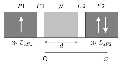
Figure 6: Sketch of an $F$/$N$/$F$ junction. The magnetization of the $F2$ conductor can be up or down, giving parallel and antiparallel configurations.

Spin injection efficiencies.

The described geometry is shown in Fig. 6. The width of the nonmagnetic conductor is $d$. The two ferromagnetic layers are labeled $F1$ and $F2$. We start with a generic asymmetric configuration in which $F1$ and $F2$ are different. Going through similar steps as in the $F$/$N$ junction, we find that the spin current polarizations in the ferromagnets at $x=0$ and $x=d$ are

$$P_{jF1}(0) = P_{\sigma F1}+\frac{1}{j}\frac{\mu_{sF1}(0)}{R_{F1}},$$ (123)

$$P_{jF2}(d) = P_{\sigma F2}-\frac{1}{j}\frac{\mu_{sF2}(d)}{R_{F2}}.$$ (124)

Similarly, at the two contacts we have

$$P_{jc1} = P_{\Sigma 1}+\frac{1}{j}\frac{\Delta\mu_{s}(0)}{R_{c1}},$$ (125)

$$P_{jc2} = P_{\Sigma 2}+\frac{1}{j}\frac{\Delta\mu_{s}(d)}{R_{c2}}.$$ (126)

In contrast to the $F$/$N$ junction, the $N$ region is of finite width $d$. Considering the quasichemical potentials $\mu_{sN}(0)$ and $\mu_{sN}(d)$ as yet unknown boundary conditions, the solution to the diffusion equation 67 is

$$\mu_{sN}(x)=\mu_{sN}(d)\frac{\sinh(x/L_{sN})}{\sinh(d/L_{sN})}-\mu_{sN}(0)\frac{\sinh\left[(x-d)/L_{sN}\right]}{\sinh(d/L_{sN})}.$$ (127)

By evaluating $\nabla\mu_{sN}(0)$ and $\nabla\mu_{sN}(d)$ from the above equation, we obtain for the spin current polarizations in the nonmagnetic region,

$$P_{jN}(0) = \frac{1}{jR_{N}}\frac{1}{\sinh(d/L_{sN})}\left[\mu_{sN}(d)-\mu_{sN}(0)\cosh(d/L_{sN})\right],$$ (128)

$$P_{jN}(d) = \frac{1}{jR_{N}}\frac{1}{\sinh(d/L_{sN})}\left[\mu_{sN}(d)\cosh(d/L_{sN})-\mu_{sN}(0)\right].$$ (129)

The above equations for the spin current polarizations need to be supplemented by the continuity conditions for the spin currents at the two contacts:

$$P_{j1}\equiv P_{jF1}(0)=P_{jc1}=P_{jN}(0),$$ (130)

$$P_{j2}\equiv P_{jF2}(d)=P_{jc2}=P_{jN}(d).$$ (131)

The algebraic system is now complete and we can solve it to obtain the spin injection efficiencies $P_{j1}$ and $P_{j2}$ at the two junctions $F1$/$N$ and $N$/$F2$:

$$P_{j1} = P_{j1}^{0}R_{1}\frac{R_{N}\coth(d/L_{sN})+R_{c2}+R_{F2}}{D_{0}}+P_{j2}^{0}\frac{R_{2}R_{N}}{D_{0}\sinh(d/L_{sN})},$$ (132)

$$P_{j2} = P_{j2}^{0}R_{2}\frac{R_{N}\coth(d/L_{sN})+R_{c1}+R_{F1}}{D_{0}}+P_{j1}^{0}\frac{R_{1}R_{N}}{D_{0}\sinh(d/L_{sN})}.$$ (133)

Here

$$D_{0}=R_{N}^{2}+(R_{c1}+R_{F1})(R_{c2}+R_{F2})+R_{N}(R_{c1}+R_{F1}+R_{c2}+R_{F2})\coth(d/L_{sN}),$$ (134)

and $P_{j1}^{0}$ and $P_{j2}^{0}$ are the spin injection efficiencies of the individual junctions giving by Eq. 87; similarly $R_{1}$ and $R_{2}$ are the two effective junction resistances:

$$R_{1}=R_{F1}+R_{c1}+R_{N},\quad R_{2}=R_{F2}+R_{c2}+R_{N}.$$ (135)

For a thick $N$ region, if $d\gg L_{sN}$, we recover the spin injection efficiencies of the individual junctions: $P_{j1}\approx P_{j1}^{0}$ and $P_{j2}\approx{P}_{j2}^{0}$, as expected for spin uncoupled contacts. In the opposite limit of a thin $N$, if $d\ll L_{sN}$,

$$P_{j1}=P_{j2}=\frac{{P}_{j1}^{0}R_{1}+{P}_{j2}^{0}R_{2}}{R_{c1}+R_{F1}+R_{c2}+R_{F2}}.$$ (136)

The spin injection efficiencies are a weighted mixture of the efficiencies of the two individual junctions. Finally, for tunnel contacts, such as $R_{c}\gg R_{N}$, $R_{F}$, and $R_{N}(L_{s}/a)$, we recover the limit of independent junctions, $P_{j1}\approx{P}_{j1}^{0}$ and $P_{j2}\approx{P}_{j2}^{0}$.

Nonequilibrium resistance.

In order to find the value of the nonequilibrium resistance due to the spin bottleneck, we need to find the increase of the quasichemical potential $\Delta\mu$ across the junction:

$${\rm emf}=\mu_{F2}(\infty)-\mu_{F1}(-\infty)=j{\cal R}+j\delta{\cal R},$$ (137)

where

$${\cal R}={\cal R}_{F1}+{\cal R}_{c1}+{\cal R}_{N}+{\cal R}_{c2}+{\cal R}_{F2},$$ (138)

is the electrical resistance of the junction in the absence of spin accumulation.

Let us apply Eq. 71 to the five regions of the $F$/$N$/$F$ junction: $F1$, $C1$, $N$, $C2$, and $F2$. In this sequence, the regional increases of the quasichemical potential are

$$\mu_{F1}(0)-\mu_{F1}(-\infty) = j{\cal R}_{F1}-P_{\sigma F1}\mu_{sF1}(0),$$ (139)

$$\mu_{N}(0)-\mu_{F1}(0) = j{\cal R}_{c1}-P_{\Sigma 1}\Delta\mu_{s}(0),$$ (140)

$$\mu_{N}(d)-\mu_{N}(0) = j{\cal R}_{N},$$ (141)

$$\mu_{F2}(d)-\mu_{N}(d) = j{\cal R}_{c2}-P_{\Sigma 2}\Delta\mu_{s}(d),$$ (142)

$$\mu_{F2}(\infty)-\mu_{F2}(d) = j{\cal R}_{F2}+P_{\sigma F2}\mu_{sF2}(d).$$ (143)

We have used that $\mu_{sF1}(-\infty)=\mu_{sF2}(\infty)=0$. Summing these equations up we extract

$$j\delta{\cal R}=-P_{\sigma F1}\mu_{sF1}(0)-P_{\Sigma 1}\Delta\mu_{s}(0)-P_{\Sigma 2}\Delta\mu_{s}(d)+P_{\sigma F2}\mu_{sF2}(d).$$ (144)

Expressing the spin chemical potentials in terms of the spin injection efficiencies $P_{j1}$ and $P_{j2}$,

$$\mu_{sF1}(0) = (P_{j1}-P_{\sigma F1})jR_{F1},$$ (145)

$$\Delta\mu_{s}(0) = (P_{j1}-P_{\Sigma 1})jR_{c1},$$ (146)

$$\Delta\mu_{s}(d) = (P_{j2}-P_{\Sigma 2})jR_{c2},$$ (147)

$$\mu_{sF2}(d) = (P_{\sigma F2}-P_{j2})jR_{F2},$$ (148)

we find for the nonequilibrium resistance

$$\delta R=-P_{\sigma F1}(P_{j1}-P_{\sigma F1})R_{F1}-P_{\Sigma 1}(P_{j1}-P_{\Sigma 1})R_{c1}-P_{\Sigma 2}(P_{j2}-P_{\Sigma 2})R_{c2}-P_{\sigma F2}(P_{j2}-P_{\sigma F2})R_{F2}.$$ (149)

Resistance difference $\Delta{\cal R}$.

Denoting as

$$\Delta P_{j} \equiv P_{j}^{\uparrow\downarrow}-P_{j}^{\uparrow\uparrow},$$ (150)

$$\Delta^{+}P_{j} \equiv P_{j}^{\uparrow\downarrow}+P_{j}^{\uparrow\uparrow},$$ (151)

the difference and the sum of the spin injection efficiencies for antiparallel and parallel magnetizations of the two ferromagnets, we find (assuming that the spin efficiencies are positive, for example)

$$\Delta{\cal R}=-(R_{F1}P_{\sigma F1}+R_{c1}P_{\Sigma 1})\Delta P_{j1}-(R_{F2}P_{\sigma F2}+R_{c1}P_{\Sigma 2})\Delta^{+}P_{j2}.$$ (152)

From Eqs. 132 and 133 we find

$$\Delta P_{j1} = -2\frac{R_{2}R_{N}}{D_{0}\sinh(d/L_{sN})}{P}_{j2}^{0},$$ (153)

$$\Delta^{+}P_{j2} = -2\frac{R_{1}R_{N}}{D_{0}\sinh(d/L_{sN})}{P}_{j1}^{0}.$$ (154)

With that we finally get our desired result,

$$\Delta{\cal R}=\frac{4R_{1}R_{2}}{D_{0}\sinh(d/L_{sN})}R_{N}|{P}_{j1}^{0}P_{j2}^{0}|.$$ (155)

As expected, $\Delta{\cal R}$ vanishes exponentially if $d\gg L_{sN}$, as the differences between parallel and antiparallel cases diminish. On the other hand, for $d\ll L_{sN}$,

$$\Delta{\cal R}\approx\frac{4R_{1}R_{2}}{R_{F1}+R_{c1}+R_{c2}+R_{F2}}P_{j1}^{0}P_{j2}^{0}.$$ (156)

Transparent contacts.

Put $R_{c1}=R_{c2}=0$ and consider the interesting case of a thin $N$ layer, $d\ll L_{sN}$. For simplicity assume the same ferromagnets, $R_{F1}=R_{F2}$. Then

$$\delta{\cal R}\approx 2R_{F}P_{\sigma F}^{2}.$$ (157)

Problem. Analyze $\Delta{\cal R}$ in Eq. 156 in the conductivity mismatch regime, $R_{N}\gg R_{c}$, $R_{F}$.

Tunnel contacts.

Suppose now that the most resistive regions are the contacts and the $N$ region is thin, $d\ll L_{sN}$. Assuming a symmetric junction, the nonequilibrium resistance difference is

$$\Delta{\cal R}\approx\frac{2R_{c}P_{\sigma}^{2}}{1+(R_{c}/R_{N})(d/2L_{sN})}.$$ (158)

The spin accumulation detection by $\Delta R$ will be most sensitive if

$$dR_{c}\ll L_{sN}R_{N},$$ (159)

as then $\Delta{\cal R}\approx R_{c}$ and the resistance change is maximized. Let us find the physical meaning of the above inequality by invoking the definition of $R_{N}$, the diffusion length $L_{sN}$, and the Einstein relation:

$$1\gg\frac{dr_{c}}{r_{N}L_{sN}}=\frac{d}{L_{sN}^{2}}r_{c}\sigma_{N}=\frac{d}{D_{N}\tau_{sN}}r_{c}e^{2}g_{N}D_{N}\approx e^{2}(dg_{N})\frac{1}{\Sigma_{c}}\frac{1}{\tau_{s}}.$$ (160)

Expressing the tunnel conductance $\Sigma_{c}$ through an effective tunneling probability per unit time, $P_{\rm tunnel}$,

$$\Sigma_{c}=e(dg_{N})P_{\rm tunnel},$$ (161)

and introducing the dwell time

$$\tau_{\rm dwell}=1/P_{\rm tunnel},$$ (162)

we come to the conclusion that the spin accumulation detection in $F$/$N$/$F$ tunnel junctions is most efficient if

$$\tau_{\rm dwell}\ll\tau_{sN}.$$ (163)

In words, the dwell time of the electrons in between the two tunnel barriers (the average time the electron spends in the $N$ region) must be much smaller than the spin relaxation time.

Problem. $N$/$F$/$N$ junction. Calculate the spin efficiency $P_{j}$ and the nonequilibrium resistance $\delta{\cal R}$ for a symmetric $N$/$F$/$N$ junction.
a) Show that in the limit of a thin $F$ layer ($d\ll L_{sF}$)

$$P_{j} = \frac{R_{c}P_{\Sigma}}{R_{c}+R_{N}},$$ (164)

$$\delta{\cal R} = \frac{2R_{c}R_{N}P_{\Sigma}^{2}}{R_{c}+R_{N}}.$$ (165)

b) Verify that in the limit of a thick $F$ layer ($d\gg L_{sF}$) the spin injection efficiency $P_{j}$ reduces to its value for a single $F$/$N$ junction, and that $\delta{\cal R}$ of an $N$/$F$/$N$ junction is twice the nonequilibrium resistance of the individual $F$/$N$ junctions.

9 Nonlocal spin-injection geometry: Johnson-Silsbee spin injection experiment.

In the $F$/$N$/$F$ junction studied in the previous section the electric current flows through both contacts. As the current often brings spurious effects from the point of view of spin detection, especially in the presence of an external magnetic field (the Hall effect or anisotropic magnetoresistance), it is important to consider spin injection geometries in which the spin detection circuit is open. We have already met one example of an open circuit spin detection: the Silsbee-Johnson spin-charge coupling. This scheme can be naturally extended to include a spin injection contact, giving what is called a nonlocal spin-injection geometry (as the injection and detection circuits are independent) or the Johnson-Silsbee spin injection experiment, after the original spin injection scheme.

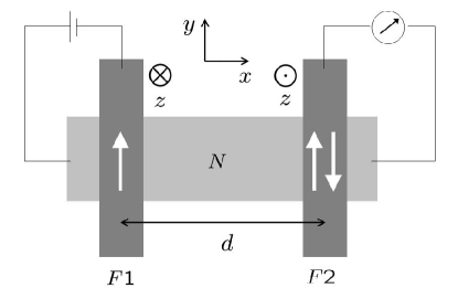
Figure 7: Nonlocal geometry for spin injection and detection. The $F1$/$N$ circuit is closed, the $F2$/$N$ is open; the electrode $F1$ acts as a spin source, $F2$ as a spin drain. The axes labels are indicated. The directions of the $z$ axis are opposite for the two junctions.

Our goal is to answer the following question:

Suppose electric current drives spin injection in the spin injection circuit $F1$/$N$ as indicated in Fig. 7. What is the emf in the open $F2$/$N$ junction?

The two ferromagnetic electrodes are on the top of a nonmagnetic conductor, separated by spin-polarizing contacts. Spin is injected into $N$ from $F1$. While the electric current flows in the closed circuit formed by $F1$/$N$, the spin current flows also towards the spin detection circuit $N$/$F2$. The charge and spin flows are indicated in Fig. 8. For spin the contact $F1$/$N$ acts as a spin source, while $N$/$F2$ as a spin sink. The source and sink will appear as special boundary conditions for the spin transport in $N$. The axes labels are defined in Fig. 7.

We need to be a little careful with this geometry since in principle we are now dealing with a two (if not three) dimensional problem. Nevertheless, the problem can be decoupled to one-dimensional ones if we assume, realistically, that the dimensions of the ferromagnetic electrodes are much greater than the spin diffusion length in the ferromagnets. Indeed, a representative $L_{sF}$ would be on the order of 10 nm or so. In that case we can consider the spin current in $F1$ and $F2$ one-dimensional, along $z$. On the other hand, we assume that the contact dimensions between $F$ and $N$, as well as the thickness of $N$, are much smaller than the spin diffusion length in the non-magnetic conductor, so that the spin current in $N$ can be considered one-dimensional as well. Typically $L_{sN}$ would be more than 1 $\mu$m. In most other cases one would need to set up a two-dimensional drift-diffusion problem.

With the above physical restrictions, the quantities labeled $N$ vary along $x$, while those of $F_{1}$ and $F_{2}$ along $z$, as indicated in Figs. 7 and 8. For example, if we write $\mu_{sF2}(0)$ we mean $\mu_{sF2}(z=0)$, the value of the spin quasichemical potential in $F2$ at the place of contact with $N$. Any variation of $\mu_{sF2}$ along $y$ or $x$ is insignificant, occurring at the contact edges only.

We now apply the boundary conditions for the spin quasichemical potentials $\mu_{s}$ at infinities:

$$\mu_{sN}(\pm\infty)=\mu_{sF1}(-\infty)=\mu_{sF2}(\infty)=0.$$ (166)

Let us consider each junction separately.

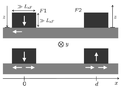
Figure 8: Cross view of the nonlocal geometry. The upper graph indicates the flow of electrons, the lower graphs shows the flow of spins. From the point of view of the spin flow in $N$, the injector plays a role of a spin source, while the detector acts as a spin sink, taking away some of the spin current.

Spin injector: $F1$/$N$ junction.

The distribution of the spin currents is shown in Fig. 8. In $F1$ the spin accumulation has the profile

$$\mu_{sF1}(z)=\mu_{sF1}(0)e^{z/L_{sF2}},$$ (167)

giving for the spin current at the contact, using Eq. 52

$$j_{sF1}(0)=jP_{\sigma F1}+\frac{1}{R_{F1}}\mu_{sF1}(0).$$ (168)

The spin current through the spin-polarizing contact $C1$ is

$$j_{sc1}=jP_{\Sigma 1}+\frac{1}{R_{c1}}\left[\mu_{sN}(0)-\mu_{sF1}(0)\right].$$ (169)

To obtain the spin current in $N$, we need to know the profile of the spin quasichemical potential $\mu_{sN}$. Treating the chemical potential at $x=0$ and $x=d$ as yet unknown, the profile is given by Eq. 127 for $x>0$. The profile in the whole $N$ region is

$$\mu_{sN}(x\leq 0) = \mu_{sN}(0)e^{x/L_{sN}},$$ (170)

$$\mu_{sN}(0<x<d) = \mu_{sN}(d)\frac{\sinh(x/L_{sN})}{\sinh(d/L_{sN})}-\mu_{sN}(0)\frac{\sinh\left[(x-d)/L_{sN}\right]}{\sinh(d/L_{sN})},$$ (171)

$$\mu_{sN}(x\geq d) = \mu_{sN}(d)e^{-x/L_{sN}}.$$ (172)

The spin current is not continuous at $x=0$, due to the presence of the spin source:

$$j_{sN}(0+) = \frac{1}{R_{N}}\left[-\mu_{sN}(0)\coth\left(d/L_{sN}\right)+\frac{\mu_{sN}(d)}{\sinh\left(d/L_{sN}\right)}\right],$$ (173)

$$j_{sN}(0-) = \frac{1}{R_{N}}\mu_{sN}(0).$$ (174)

The continuity of the spin current at the contact requires that

$$j_{sN}(0+)=j_{sN}(0-)+j_{sc1}=j_{sN}(0-)+j_{sF1}.$$ (175)

Using the above algebraic system, we find

$$\mu_{sN}(0)\left[\frac{R_{N}}{R_{c1}+R_{F1}}+\frac{\exp\left(d/L_{sN}\right)}{\sinh\left(d/L_{sN}\right)}\right]-\mu_{sN}(d)\frac{1}{\sinh\left(d/L_{sN}\right)}=-jR_{N}\frac{P_{\Sigma 1}R_{c1}+P_{\sigma F1}R_{F1}}{R_{c1}+R_{F1}}.$$ (176)

The spin current in the spin injector contact is

$$j_{sF1}=j\frac{P_{\Sigma 1}R_{c1}+P_{\sigma F1}R_{F1}+\mu_{sN}(0)/j}{R_{c1}+R_{F1}}.$$ (177)

Finally, we define the spin injection efficiency for the spin injector in the nonlocal geometry as

$$P_{j1}=\frac{j_{sN}(0+)}{j}.$$ (178)

Only the spin current which gives rise to the spin accumulation at the detector circuit is relevant.

Spin detector: $F2$/$N$ junction.

There is no electric current flowing in the spin detector: $j=0$. The flow of spin is indicated in Fig. 8. Similarly to the $F1$/$N$ junction, we obtain for the spin currents in the ferromagnet and the contact,

$$j_{sF2}(0) = -\frac{1}{R_{F2}}\mu_{sF2}(0),$$ (179)

$$j_{sc2} = \frac{1}{R_{c2}}\left[\mu_{sF2}(0)-\mu_{sN}(d)\right].$$ (180)

The spin current along $x$ is again discontinuous at $x=d$, due to the presence of the spin sink:

$$j_{sN}(d-) = \frac{1}{R_{N}}\left[-\frac{\mu_{sN}(0)}{\sinh\left(d/L_{sN}\right)}+\mu_{sN}(d)\coth\left(d/L_{sN}\right)\right],$$ (181)

$$j_{sN}(d+) = -\frac{1}{R_{N}}\mu_{sN}(d).$$ (182)

The continuity for the spin currents at $x=d$ gives

$$j_{sN}(d-)=j_{sN}(d+)+j_{sc2}=j_{sN}(d+)+j_{sF2}(0).$$ (184)

Solving the above algebraic system yields

$$\mu_{sN}(0)\frac{1}{\sinh\left(d/L_{sN}\right)}-\mu_{sN}(d)\left[\frac{R_{N}}{R_{c2}+R_{F2}}+\frac{\exp\left(d/L_{sN}\right)}{\sinh\left(d/L_{sN}\right)}\right]=0.$$ (185)

Let us denote the spin current in the contact as $j_{s2}$:

$$j_{s2}\equiv j_{sc2}=j_{sF2}(0).$$ (186)

We will need to know the value of this current to calculate the emf at the detector circuit. We find that

$$j_{s2}=-\frac{\mu_{sN}(d)}{R_{c2}+R_{F2}}.$$ (187)

Spin quasichemical potentials.

Equations 176 and 185 form a closed system, allowing us to extract the spin quasichemical potentials at the two contacts:

$$\mu_{sN}(0) = -j\frac{R_{N}P_{j1}^{0}}{2}\left[1-\frac{R_{N}}{2R_{2}}\left(1+e^{-2d/L_{sN}}\right)\right]\frac{1}{\kappa},$$ (188)

$$\mu_{sN}(d) = -j\frac{R_{N}P_{j1}^{0}}{2}\left(\frac{R_{c2}+R_{F2}}{R_{2}}\right)\frac{e^{-d/L_{sN}}}{\kappa},$$ (189)

where

$$\kappa=\frac{R_{N}^{2}}{4R_{1}R_{2}}\left[\left(1+2\frac{R_{c1}+R_{F1}}{R_{N}}\right)\left(1+2\frac{R_{c2}+R_{F2}}{R_{N}}\right)-e^{-2d/L_{sN}}\right].$$ (190)

Recall that $R_{1}$ and $R_{2}$ are the total effective resistances of the two junctions; see Eqs. 135. Similarly, $P_{j1}^{0}$ and $P_{j2}^{0}$ are the spin injection efficiencies of the individual $F$/$N$ junctions, given by Eq. 87.

Problem. Calculate the spin injection efficiency $P_{j1}$ of the spin injection circuit. What do you get in the limit of $d\gg L_{sN}$? Does the result agree with that for an isolated $F$/$N$ junction studied earlier?

emf in the detector circuit.

Due to the presence of a nonequilibrium spin in the detector circuit, an emf will develop there. We can obtain it as the increase of the quasichemical potential from the far end of the $F2$ to the far right of the $N$ region, as shown in Fig. 7. Since the spin flow in $F2$ is confined to the distance of order $L_{sF2}$ from $z=0$, the quasichemical potential $\mu_{sF2}$ far away from the contact, at $y\to\pm\infty$ (we are mixing the third dimension here!) will be the same as that at the contact itself, $y\approx 0$, but at $z=\infty$:

$${\rm emf}=\mu_{N}(\infty)-\mu_{F2}(\infty).$$ (192)

Since $j=0$ in the $F2$/$N$ junction, we can write,

$$\mu_{F2}(0)-\mu_{F2}(\infty) = -P_{\sigma F2}\mu_{sF2}(0),$$ (193)

$$\mu_{N}(d)-\mu_{F2}(0) = -P_{\Sigma 2}\left[\mu_{sN}(d)-\mu_{sF2}(0)\right],$$ (194)

$$\mu_{N}(\infty)-\mu_{N}(d) = 0.$$ (195)

Summing these equations up we get, after substituting for the spin quasichemical potentials Eqs. 179 and 180,

$${\rm emf}=(R_{c2}P_{\Sigma 2}+R_{F2}P_{\sigma 2})j_{s2}.$$ (196)

This is just another realization of Silsbee-Johnson spin-charge coupling: An electromotive force develops due to the presence of a spin current in a spin-polarized contact or a ferromagnetic conductor. Due to charge neutrality this emf can be detected as a voltage drop.

Substituting for $j_{s2}$ using Eq. 187 and using Eq. 189 for $\mu_{sN}(d)$, the emf can be readily obtained:

$${\rm emf}=j\frac{R_{N}}{2}{P}_{j1}^{0}{P}_{j2}^{0}\frac{e^{-d/L_{sN}}}{\kappa}.$$ (197)

The emf is in general positive for parallel and negative for antiparallel magnetization orientations.

Often what is detected is the nonlocal resistance,

$${\cal R}_{\rm nl}=\frac{{\rm emf}}{j}=\frac{R_{N}}{2}{P}_{j1}^{0}{P}_{j2}^{0}\frac{e^{-d/L_{sN}}}{\kappa},$$ (198)

or the corresponding difference in the nonlocal resistance for parallel and antiparallel orientations of the magnetizations of $F1$ and $F2$:

$$\Delta{\cal R}_{\rm nl}={\cal R}_{\rm nl}^{\uparrow\uparrow}-{\cal R}_{\rm nl}^{\uparrow\uparrow}=2|{\cal R}_{\rm nl}|.$$ (199)

Tunnel contacts.

For tunnel contacts we find $\kappa\approx 1$ and

$${\rm emf}=j\frac{R_{N}}{2}P_{\Sigma 1}P_{\Sigma 2}e^{-d/L_{sN}},$$ (200)

as one would expect. The factor of “1/2” appears due the geometry of the spin injector: only half of the injected spin current in the $F1$/$N$ junction flows towards the $F2$/$N$ junction. The other half flows towards $x\to-\infty$.

Transparent contacts.

The most general expression for transparent contacts is the same as Eq. 197, with $R_{c1}=R_{c2}=0$. In the conductivity mismatch regime, for $R_{N}\gg R_{F1},R_{F2}$, the emf simplifies to

$${\rm emf}=2jR_{N}P_{\sigma F1}P_{\sigma F2}\left(\frac{R_{F1}R_{F2}}{R_{N}^{2}}\right)\frac{e^{-d/L_{sN}}}{1-e^{-2d/L_{sN}}}.$$ (201)

The conductivity mismatch limits the spin injection/detection in the nonlocal geometry.

Problem. Tunnel/transparent contacts. Calculate emf for the mixed case of tunnel and transparent contacts of the nonlocal spin injection geometry.

References

- [1] Aronov A G 1976 Zh. Eksp. Teor. Fiz. Pisma Red. 24 37–39 [JETP Lett. 24, 32-34 (1976)]
- [2] Johnson M and Silsbee R H 1987 Phys. Rev. B 35 4959–4972
- [3] Johnson M and Silsbee R H 1988 Phys. Rev. B 37 5312–5325
- [4] Žutić I, Fabian J and Das Sarma S 2004 Rev. Mod. Phys. 76 323–410
- [5] Fabian J, Matos-Abiague A, Ertler C, Stano P and Žutić I 2007 Acta Phys. Slov. 57 565–907
- [6] van Son P C, van Kempen H and Wyder P 1987 Phys. Rev. Lett. 58 2271–2273
- [7] Valet T and Fert A 1993 Phys. Rev. B 48 7099–7113
- [8] Fert A and Jaffres H 2001 Phys. Rev. B 64 184420
- [9] Hershfield S and Zhao H L 1997 Phys. Rev. B 56 3296–3305
- [10] Schmidt G, Ferrand D, Molenkamp L W, Filip A T and van Wees B J 2000 Phys. Rev. B 62 R4790–R4793
- [11] Fabian J, Žutić I and Das Sarma S 2002 Phys. Rev. B 66 165301
- [12] Žutić I, Fabian J and Das Sarma S 2002 Phys. Rev. Lett. 88 066603
- [13] Jedema F J, Nijboer M S, Filip A T and van Wees B J 2003 Phys. Rev. B 67 085319
- [14] Rashba E I 2000 Phys. Rev. B 62 R16267–R16270
- [15] Rashba E I 2002 Eur. Phys. J. B 29 513–527
- [16] Vignale G and D’Amico I 2003 Solid State Commun. 127 829
- [17] Jonker B T, Erwin S C, Petrou A and Petukhov A G 2003 MRS Bull. 28 740–748
- [18] Takahashi S and Maekawa S 2003 Phys. Rev. B 67 052409
- [19] Fert A, George J M, Jaffres H and Mattana R 2007 IEEE Trans. Electronic Devices 54 921–932
- [20] Žutić I, Fabian J and Erwin S C 2006 Phys. Rev. Lett. 97 026602