Surface magnetoinductive breathers in two-dimensional magnetic metamaterials

Abstract

We study discrete surface breathers in two-dimensional lattices of inductively-coupled split-ring resonators with capacitive nonlinearity. We consider both Hamiltonian and dissipative systems and analyze the properties of the modes localized in space and periodic in time (discrete breathers) located in the corners and at the edges of the lattice. We find that surface breathers in the Hamiltonian systems have lower energy than their bulk counterparts, and they are generally more stable.

Theoretical results on the existence of novel types of discrete surface solitons localized in the corners or at the edges of two-dimensional photonic lattices makris_2D ; pla_our ; pre_2D have been recently confirmed by the experimental observation of two-dimensional surface solitons in optically-induced photonic lattices prl_1 and two-dimensional waveguide arrays laser-written in fused silica prl_2 ; ol_szameit . These two-dimensional nonlinear surface modes demonstrate novel features in comparison with their counterparts in truncated one-dimensional waveguide arrays OL_george ; PRL_george ; OL_molina . In particular, in a sharp contrast to one-dimensional surface solitons, the mode threshold is lower at the surface than in a bulk making the mode excitation easier pla_our .

Recently, it was shown LTK that, similar to discrete solitons analyzed extensively for optical systems, surface discrete breathers can be excited near the edge of a one-dimensional metamaterial created by a truncated array of nonlinear split-ring resonators. Networks of split-ring resonators (SRRs) that have nonlinear capacitive elements can support nonlinear localized modes or discrete breathers (DB’s) under rather general conditions that depend primarily on the inductive coupling between SRRs and their resonant frequency LET ; ELT . The corresponding one-dimensional surface modes have somewhat lower energy (in the Hamiltonian case) and can easily be generated in one-dimensional SRR lattices LTK .

In this Brief Communication, we develop further those ideas and analyze two-dimensional lattices of split-ring resonators. Similar to the optical systems, we find that two-dimensional lattices of inductively-coupled split-ring resonators with capacitive nonlinearity can support the existence of long-lived two-dimensional discrete breathers localized in the corners or at the edge of the lattice.

We consider a two-dimensional lattice of SRRs in both planar and planar-axial configuration [see Figs. 1(a,b)]. In the planar configuration, all SRR loops are in the same plane with their centers forming an orthogonal lattice, while in the planar-axial configuration the loops have a planar arrangement in one direction and an axial configuration in the other direction. Each SRR is equivalent to a nonlinear RLC circuit, with an ohmic resistance $R$, self-inductance $L$, and capacitance $C$. We assume that the capacitor $C$ contains a nonlinear Kerr-type dielectric, so that the permittivity $\epsilon$ can be presented in the form,

$$\epsilon(|{\bf E}|^{2})=\epsilon_{0}\left(\epsilon_{\ell}+\alpha\frac{|{\bf E}|^{2}}{E_{c}^{2}}\right),$$ (1)

where ${\bf E}$ is the electric field with the characteristic value $E_{c}$, $\epsilon_{\ell}$ is linear permittivity, $\epsilon_{0}$ is the permittivity of the vacuum, and $\alpha=+1~{}~{}(-1)$ corresponding to self-focusing (self-defocusing) nonlinearity, respectively. As a result, each SRR acquires the field-dependent capacitance $C(|{\bf E}|^{2})=\epsilon(|{\bf E}_{g}|^{2})\,A/d_{g}$, where $A$ is the area of the cross-section of the SRR wire, ${\bf E}_{g}$ is the electric field induced along the SRR slit, and $d_{g}$ is the size of the slit. The field ${\bf E}_{g}$ is induced by the magnetic and/or electric component of the applied electromagnetic field, depending on the relative orientation of the field with respect to the SRR plane and the slits Shardivov . Below we assume that the magnetic component of the incident (applied) electromagnetic field is always perpendicular to the SRR plane, so that the electric field component is transverse to the slit. With this assumption, only the magnetic component of the field excites an electromotive force in SRRs, resulting in an oscillating current in each SRR loop. This results in the development of an oscillating voltage difference $U$ across the slits or, equivalently, of an oscillating electric field ${\bf E}_{g}$ in the slits.

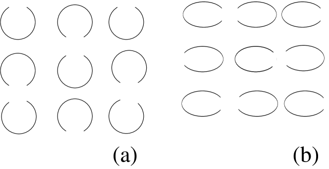
Figure 1: Schematic of a two-dimensional lattice of split-ring resonators for (a) planar and (b) planar-axial geometries. In both the geometries the magnetic component of the applied field is directed along the SRR axes, while the electric field component is transverse to the slits.

If $Q$ is a charge stored in teach SRR capacitor, from a general relation of a voltage-dependent capacitance $C(U)=dQ/dU$ and Eq. (1), we obtain

$$Q=C_{\ell}\left(1+\alpha\frac{U^{2}}{3\epsilon_{\ell}\,U_{c}^{2}}\right)U,$$ (2)

where $U=d_{g}E_{g}$, $C_{\ell}=\epsilon_{0}\epsilon_{\ell}(A/d_{g})$ is the linear capacitance, and $U_{c}=d_{g}E_{c}$. We assume that the arrays are placed in a time-varying and spatially uniform magnetic field of the form

$$H=H_{0}\,\cos(\omega t),$$ (3)

where $H_{0}$ is the field amplitude, $\omega$ is the field frequency, and $t$ is the time variable. The excited electromotive force ${\cal E}$ , which is the same in all SRRs, is given by the expression

$${\cal E}={\cal E}_{0}\,\sin(\omega t),\qquad{\cal E}_{0}\equiv\mu_{0}\,\omega\,S\,H_{0},$$ (4)

where $S$ is the area of each SRR loop, and $\mu_{0}$ the permittivity of the vacuum. Each SRR exposed to the external field given by Eq. (3) is a nonlinear oscillator exhibiting a resonant magnetic response at a particular frequency which is very close to its linear resonance frequency $\omega_{\ell}=1/\sqrt{L\,C_{\ell}}$ (for $R\simeq 0$).

All SRRs in an array are coupled together due to magnetic dipole-dipole interaction through their mutual inductances. However, we assume below only the nearest-neighbor interactions, so that neighboring SRRs are coupled through their mutual inductances $M_{x}$ and $M_{y}$. This is a good approximation in the planar configurations [see Fig.1(a)], even if SRRs are located very close. Validity of the nearest-neighbor approximation for the planar-axial configuration [see Fig.1(b)] has been verified by taking into account the interaction of SRRs with their four nearest neighbors. Assumimg that the mutual inductance $M_{x,y}^{(s)}$ between an SRR and its $s-$th neighbor decays with distance as $M_{x,y}^{(s)}\simeq M_{x,y}/s^{3}$  ELT , we find practically the same results. Therefore, the electrical equivalent of an SRR array in an alternating magnetic field is an array of nonlinear RLC oscillators coupled with their nearest neighbors through their mutual inductances; the latter are being driven by identical alternating voltage sources. Equations describing the dynamics of the charge $Q_{n,m}$ and the current $I_{n,m}$ circulating in the $n,m-$th SRR may be derived from Kirchhoff’s voltage law for each SRR LET ; Shardivov

$$\frac{dQ_{n,m}}{dt} = I_{n,m}$$ (5)

$$L\frac{dI_{n,m}}{dt} + RI_{n,m}+f(Q_{n,m})=$$ (6)

$$- M_{x}\left(\frac{dI_{n-1,m}}{dt}+\frac{dI_{n+1,m}}{dt}\right)$$

$$- M_{y}\left(\frac{dI_{n,m-1}}{dt}+\frac{dI_{n,m+1}}{dt}\right)+{\cal E},$$

where $f(Q_{n,m})=U_{n,m}$ is given implicitly from Eq. (2). Using the relations

$$\omega_{\ell}^{-2} = LC_{\ell},~{}~{}\tau=t\omega_{\ell},~{}~{}I_{c}=U_{c}\omega_{\ell}C_{\ell},~{}~{}Q_{c}=C_{\ell}U_{c}$$ (7)

$${\cal E} = U_{c}\varepsilon,~{}~{}I_{n,m}=I_{c}i_{n,m},~{}~{}Q_{n,m}=Q_{c}q_{n,m},$$ (8)

and Eq. (4), we normalize Eqs. (5) and (6) to the form

$$\frac{dq_{n,m}}{d\tau} = {i_{n,m}}$$ (9)

$$\frac{di_{n,m}}{d\tau} + \gamma\,i_{n,m}+f(q_{n,m})+\lambda_{x}\left(\frac{di_{n-1,m}}{d\tau}+\frac{di_{n+1,m}}{d\tau}\right)$$ (10)

$$+ \lambda_{y}\left(\frac{di_{n,m-1}}{d\tau}+\frac{di_{n,m+1}}{d\tau}\right)=\varepsilon_{0}\,\sin(\Omega\tau),$$

where $\gamma=RC_{\ell}\omega_{\ell}$ is the loss coefficient, $\lambda_{x,y}=M_{x,y}/L$ are the the coupling parameters in the $x-$ and $y-$direction, respectively, and $\varepsilon_{0}={\cal E}_{0}/U_{c}$. Note that the loss coefficient $\gamma$, which is usually small ($\gamma\ll 1$), may account both for Ohmic and radiative losses Kourakis . Neglecting losses and without applied field, Eqs. (9) and (10) can be derived from the Hamiltonian

$${\cal H} = \sum_{n,m}\left\{\frac{1}{2}\dot{q}_{n,m}^{2}+V_{n,m}\right\}$$ (11)

$$- \sum_{n,m}\left\{\lambda_{x}\,\dot{q}_{n,m}\,\dot{q}_{n+1,m}+\lambda_{y}\,\dot{q}_{n,m}\,\dot{q}_{n,m+1}\right\},$$

where the nonlinear on-site potential $V_{n,m}$ is given by

$$V_{n,m}\equiv V(q_{n,m})=\int_{0}^{q_{n,m}}f(q_{n,m}^{\prime})\,dq_{n,m}^{\prime},$$ (12)

and $\dot{q}_{n,m}\equiv d{q}_{n,m}/d\tau$. Analytical solution of Eq. (2) for $u_{n,m}=f(q_{n,m})$ with the conditions of $u_{n,m}$ being real and $u_{n,m}(q_{n,m}=0)=0$, gives the approximate expression

$$f(q_{n,m})\simeq q_{n,m}-\frac{\alpha}{3\epsilon_{\ell}}q_{n,m}^{3}+3\left(\frac{\alpha}{3\epsilon_{\ell}}\right)^{2}q_{n,m}^{5},$$ (13)

which is valid for relatively low $q_{n}$ ($q_{n}<1,~{}~{}n=1,2,...,N$). Thus, the on-site potential is soft for $\alpha=+1$ and hard for $\alpha=-1$. In the 2D case the mutual inductances $M_{x}$ and $M_{y}$ may differ both in their sign, depending on the configuration, and their magnitude. Actually, even in the planar 2D configuration with $d_{x}=d_{y}$ a small anisotropy should be expected because we consider SRRs having only one slit. This anisotropy can be effectively taken into account by considering slightly different coupling parameters $\lambda_{x}$ and $\lambda_{y}$. The coupling parameters $\lambda_{x,y}$ as well as the loss coefficient $\gamma$ can be calculated numerically for this specific model with high accuracy. However, for our purposes, it is sufficient to estimate these parameters for realistic (experimental) array parameters, ignoring the nonlinearity of the SRRs and the effects due to the weak coupling as in Refs. LET ; ELT with the following typical values $\lambda\approx 0.02$ and $\gamma\approx 0.01$.

We construct discrete breathers located in the corner of a two-dimensional lattice of $15\times 15$ sites using the anti-continuous limit method as in Ref.  LET for the set of Eqs. (9)-(10), setting $\gamma=0$ and $\varepsilon_{0}=0$ (Hamiltonian discrete breathers). For the case of $\alpha=+1$ corresponding to self-focusing nonlinearity and period $T_{b}=6.69$, we may construct linearly stable breathers for parameters up to $\lambda_{x}=\lambda_{y}=0.029$. Breather stability has been checked through the Floquet monodromy matrix throughout the paper. For the case where an anisotropy is introduced, $\lambda_{x}<\lambda_{y}$, linearly stable discrete breathers can be constructed up to $\lambda_{x}=0.028$ and simultaneously $\lambda_{y}=0.031$, or for the case of planar-axial configuration up to $\lambda_{x}=0.031$ and at the same time $\lambda_{y}=-0.028$. If we look for discrete breathers constructed in the middle of the upper edge of the lattice for example, we find that the values of the coupling where an instability occurs are slightly decreased (e.g. the upper stability limit of coupling for planar geometry is $\lambda_{x}=\lambda_{y}=0.028$). Several cases of linearly stable discrete breathers are shown in Fig. 2 for $\alpha=+1$. The same analysis holds for $\alpha=-1$ (defocusing nonlinearity) where the upper stability limit for the values of couplings are of the same order of magnitude as for $\alpha=+1$, both for the corner and edge breathers (see Fig. 3). The breather period in the latter case is $T_{b}=5.8$.

Figure 2: Density amplitudes $q_{n,m}$ for discrete Hamiltonian breathers constructed in (a-c) upper left corner or (d-f) upper edge of the lattice of $15\times 15$ sites, $\alpha=+1$ and $T_{b}=6.69$. (a,c) $\lambda_{x}=\lambda_{y}=0.028$, (b,e) $\lambda_{x}=0.026$ and $\lambda_{y}=0.029$, (c,f) $\lambda_{x}=0.029$ and $\lambda_{y}=-0.026$. All plots depict a $5\times 5$ sublattice that includes the breather zones.

Figure 3: Density amplitude $q_{n,m}$ for discrete Hamiltonian breathers constructed in (a-c) upper left corner or in (d-f) upper edge of a lattice of $15\times 15$ sites, $\alpha=-1$ and $T_{b}=5.8$. (a,d) $\lambda_{x}=\lambda_{y}=0.030$, (b,e) $\lambda_{x}=0.028$ and $\lambda_{y}=0.031$, (c,f) $\lambda_{x}=0.028$ and $\lambda_{y}=-0.025$. All plots depict the $5\times 5$ sublattice around the linearly stable breathers.

Localized modes in the damped-driven case are constructed for $\gamma=0.01$, $\varepsilon_{0}=0.04$ and $\alpha=+1$ with the method described in Ref. LET . The resulting localized modes are called dissipative breathers, and their examples are shown in Fig. 4 for $T_{b}=5.8$ and (a) $\lambda_{x}=\lambda_{y}=0.0007$, (b) $\lambda_{x}=0.0022$ and $\lambda_{y}=0.0052$, and (c) $\lambda_{x}=0.0052$ and $\lambda_{y}=-0.0022$. The dissipative modes have been evolved in time, and we found that at long times some dissipative breathers constructed for relatively large couplings loose their initial shape and finally decay.

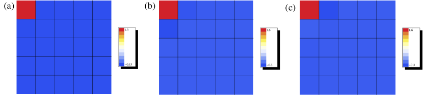
Figure 4: Density amplitude $q_{n,m}$ for discrete dissipative breathers for $\gamma=0.01$, $\varepsilon_{0}=0.04$, $\alpha=+1$ and $T_{b}=6.82$, constructed in the upper left corner for (a) $\lambda_{x}=\lambda_{y}=0.0007$, (b) $\lambda_{x}=0.0022$ and $\lambda_{y}=0.0052$, and (c) $\lambda_{x}=0.0052$ and $\lambda_{y}=-0.0022$. All plots depict the $5\times 5$ sublattice around the breather. Dissipative breathers are very narrow and essentially confined on one lattice site.

Additionally, we calculate the total energy of discrete breathers in a lattice with planar and planar-axial configuration for $\alpha=+1$ and $T_{b}=6.69$ (Hamiltonian case). Figure 5 shows the energy histograms of the relevant corner of the lattice normalized to the energy of the corner $(1,1)$ breather. In order to construct the histograms centered in each of the lattice sites, we normalized it to the edge breather energy. In the case (a) the discrete breather is constructed in a lattice of coupling $\lambda_{x}=\lambda_{y}=0.028$, in (b) the case with anisotropy in couplings $\lambda_{x}=0.026$ and $\lambda_{y}=0.029$, while in the case (c), couplings are $\lambda_{x}=0.029$ and $\lambda_{y}=-0.026$. The energy of the discrete breathers as a function of the lattice site increases, i.e, as the discrete breather is constructed in the interior of the lattice energy is larger compared to the discrete breather that is located in the corner of the lattice.

Figure 5: Histogram of the breather Hamiltonian. Breather difference energies $\Delta E$ for $\alpha=+1$, $Tb=6.69$ constructed in the upper left $3\times 3$ corner of the lattice. Case (a) $\lambda_{x}=\lambda_{y}=0.028$, case (b) $\lambda_{x}=0.026$ and $\lambda_{y}=0.029$, and case (c) $\lambda_{x}=0.029$ and $\lambda_{y}=-0.026$. To evaluate $\Delta E$ we calculate the energy of the breathers centered at different sites and subtract the energy of the corner breather.

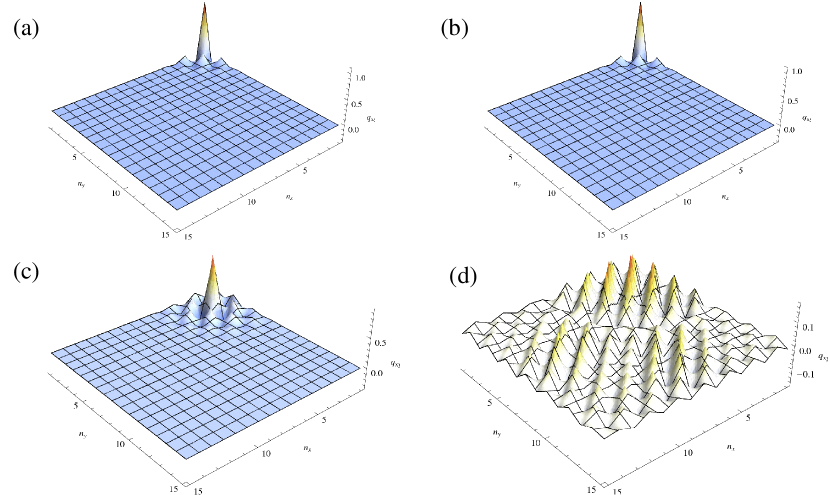
Figure 6: Amplitudes $q_{n,m}$ of the breather for $\alpha=+1$, $T_{b}=6.69$ and $\lambda_{x}=\lambda_{y}=0.028$, constructed on the site (1,1) for (a) t=0 and (b) $t=1450T_{b}$, and the breather constructed on site (3,3), for (c) $t=0$ and (d) $t=1450T_{b}$.

We note that in the one-dimensional case the bulk breathers have lower energy compared to the surface ones LTK while in two-dimensional lattice the behavior is the contrary. We thus find that two-dimensional surface and especially edge breathers form easier.

Finally, we study the time evolution of the discrete breather that is constructed in the corner site (1,1) and compare this case with a discrete breather centered at the (3,3) site for the coupling $\lambda_{x}=\lambda_{y}=0.028$. The breather of the latter case after $t=95T_{b}$ starts to loose its shape, in contrast to the breather of (1,1) site which survives for much longer times, viz. $t=1450T_{b}$ [see Fig. (6)]. For different coupling values such as $\lambda_{x}=\lambda_{y}=0.01$ we find that both the corner (1,1) and inner (3,3) breathers remain stable for at least $t=1450T_{b}$. This feature, while compatible with the fact that the corner breathers are more stable than inner ones, shows additionally that in finite lattices small changes in parameters may affect the stability properties of the breathers Morgante .

In conclusion, we have studied surface discrete breathers located in the corner and at the edge of the two-dimensional lattices of the split-ring resonators. Using standard numerical methods, we have found nonlinear localized modes both in the Hamiltonian and dissipative systems. Two-dimensional breathers in conservative lattices have been found to be linearly stable for up to certain (large) values of the coupling coefficient, in both planar and planar-axial configurations of the split-ring-resonator lattices. Dissipative discrete surface breather can retain their shapes for several periods of time, and they depending critically on the lattice coupling. Finally, we have found that the discrete breathers located deep inside the lattice have higher energy compared to the breathers located in the corners and at the edges. This distinct two-dimensional feature of nonlinear localized modes contrasts with the one-dimensional behavior being attributed to the larger number of neighbors of the two-dimensional lattice. Furthermore, the two-dimensional breathers located inside the lattice loose rapidly their initial shape as they evolve in time while the surface breathers are seen to be stable at least for $t\approx 1500T_{b}$.

References

- (1) K.G. Makris, J. Hudock, D.N. Christodoulides, G. Stegeman, O. Manela, and M. Segev, Opt. Lett. 31, 2774 (2006).
- (2) R.A. Vicencio, S. Flach, M.I. Molina, and Yu.S. Kivshar, Phys. Lett. A 364, 274 (2007).
- (3) H. Susanto, P.G. Kevrekidis, B.A. Malomed, R. Carretero-González, and D.J. Franzeskakis, Phys. Rev. E 75, 056605 (2007).
- (4) X. Wang, A. Bezryadina, Z. Chen, K.G. Makris, D.N. Christodoulides, and G.I. Stegeman, Phys. Rev. Lett. 98, 123903 (2007).
- (5) A. Szameit, Y.V. Kartashov, F. Dreisow, T. Pertsch, S. Nolte, A. Tünnermann, and L. Torner, Phys. Rev. Lett. 98, 173903 (2007).
- (6) A. Szameit, Y. V. Kartashov, V.A. Vysloukh, M. Heinrich, F. Dreisow, T. Pertsch, S. Nolte, A. Tünnermann, F. Lederer, and L. Torner, Opt. Lett. 33, 1542 (2008).
- (7) K.G. Makris, S. Suntsov, D.N. Christodoulides, G.I. Stegeman, and A. Haché, Opt. Lett. 30, 2466 (2005).
- (8) S. Suntsov, K.G. Makris, D.N. Christodoulides, G.I. Stegeman, A. Haché, R. Morandotti, H. Yang, G. Salamo, and M. Sorel, Phys. Rev. Lett. 96, 063901 (2006).
- (9) M. Molina, R. Vicencio, and Yu. S. Kivshar, Opt. Lett. 31, 1693 (2006).
- (10) N. Lazarides, G.P. Tsironis and Yu. S. Kivshar, Phys. Rev. E 77, 065601 (2008).
- (11) N. Lazarides, M. Eleftheriou, and G.P. Tsironis, Phys. Rev. Lett. 97, 157406 (2006).
- (12) M. Eleftheriou, N. Lazarides and G.P. Tsironis, Phys. Rev. E. 77, 036608 (2008).
- (13) A. A. Zharov, I. V. Shardivov and Y. S. Kivshar, Phys. Rev. Lett. 91, 037401 (2003); I. V. Shadrivov, A. A. Zharov, N. A. Zharova, and Y. S. Kivshar, Photonics Nanostruct. Fundam. Appl. 4, 69 (2006).
- (14) I. Kourakis, N. Lazarides, and G.P. Tsironis, Phys. Rev. E 75, 067601 (2007).
- (15) A. M. Morgante, M. Johansson, S. Aubry, and G. Kopidakis, J. Phys. A: Math. Gen. 35, 4999 (2002).