Investigation of nodal domains in the chaotic microwave ray-splitting rough billiard

Abstract

We study experimentally nodal domains of wave functions (electric field distributions) lying in the regime of Shnirelman ergodicity in the chaotic microwave half-circular ray-splitting rough billiard. For this aim the wave functions $\Psi_{N}$ of the billiard were measured up to the level number $N=415$. We show that in the regime of Shnirelman ergodicity ($N>208$) wave functions of the chaotic half-circular microwave ray-splitting rough billiard are extended over the whole energy surface and the amplitude distributions are Gaussian. For such ergodic wave functions the dependence of the number of nodal domains $\aleph_{N}$ on the level number $N$ was found. We show that in the limit $N\rightarrow\infty$ the least squares fit of the experimental data yields $\aleph_{N}/N\simeq 0.063\pm 0.023$ that is close to the theoretical prediction $\aleph_{N}/N\simeq 0.062$. We demonstrate that for higher level numbers $N\simeq 215-415$ the variance of the mean number of nodal domains $\sigma^{2}_{N}/N$ is scattered around the theoretical limit $\sigma^{2}_{N}/N\simeq 0.05$. We also found that the distribution of the areas $s$ of nodal domains has power behavior $n_{s}\propto s^{-\tau}$, where the scaling exponent is equal to $\tau=2.14\pm 0.12$. This result is in a good agreement with the prediction of percolation theory.

In recent theoretical papers by Bogomolny and Schmit Bogomolny2002 and Blum et al. Blum2002 the distributions of the nodal domains of real wave functions $\Psi(x,y)$ in 2D quantum systems (billiards) have been considered. Nodal domains are regions where a wave function $\Psi(x,y)$ has a definite sign. The condition $\Psi(x,y)=0$ determines a set of nodal lines which separate nodal domains. Bogomolny and Schmit Bogomolny2002 have proposed a very fruitful, percolationlike, model for description of properties of the nodal domains of generic chaotic system. Using this model they have shown that the distribution of nodal domains of quantum wave functions of chaotic systems is universal. Blum et al. Blum2002 have shown that the systems with integrable and chaotic underlying classical dynamics can be distinguished by different distributions of the number of nodal domains. In this way they provided a new criterion of quantum chaos, which is not directly related to spectral statistics.

Theoretical findings of Bogomolny and Schmit Bogomolny2002 and Blum et al. Blum2002 have been recently tested in the experiment with the microwave half-circular rough billiard by Savytskyy et al. Savytskyy2004 .

In this paper we present the first experimental investigation of nodal domains of wave functions of the chaotic microwave ray-splitting rough billiard. Ray-splitting systems are a new class of chaotic systems in which the underlying classical mechanics is non-Newtonian and non-deterministic BLUM96 ; SIR97 ; BLUMEL2001 . In ray-splitting systems a wave which encounters a discontinuity in the propagation medium splits into two or more rays travelling usually away from the discontinuity. Ray splitting occurs in many fields of physics, whenever the wave length is large in comparison with the range over which the potential changes. Ideal model systems for the investigation of ray-splitting phenomena are ray-splitting billiards COUC92 ; BLUMEL2001 and microwave cavities with dielectric inserts SIR97 ; BAUCH98 ; HLUSH2000 ; Savytskyy2001 . Measurements of wave functions of ray-splitting systems are very demanding because in principle they require the direct access to the all parts of the system Stoeckmann2001 including those filled with ray-splitting media, such as dielectric in the case of ray-splitting microwave billiards. This is one of the main reasons for which only low wave functions ($N\leq 100$) of ray-splitting billiards have been measured so far Stoeckmann2001 . In this paper we use a new method of the reconstruction of wave functions introduced by Savytskyy and Sirko Savytskyy2002 which in the case of the half-circular microwave ray-splitting rough billiard allowed for the reconstruction of wave functions with the level numbers $N\leq 415$.

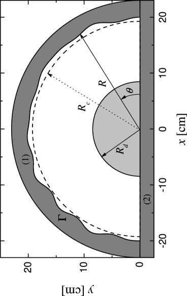
Figure 1: Sketch of the chaotic half-circular microwave ray-splitting rough billiard which consists a half-circular Teflon insert of radius $R_{d}=8.465$ cm. Dimensions are given in cm. The cavity sidewalls are marked by 1 and 2 (see text). Squared wave functions $|\Psi_{N}(R_{c},\theta)|^{2}$ were evaluated on a half-circle of fixed radius $R_{c}=19.25$ cm. Billiard’s rough boundary is marked by $\Gamma$.

In the experiment we used the thin (height $h=8$ mm) aluminium cavity in the shape of a rough half-circle (Fig. 1) which consisted a half-circular Teflon insert of radius $R_{d}=8.465$ cm. The insert had the same height as the rough cavity. The microwave cavity simulates the rough ray-splitting quantum billiard due to the equivalence between the Schrödinger equation and the Helmholtz equation BLUMEL2001 . This equivalence remains valid for frequencies less than the cut-off frequency $\nu_{c}=c/2\eta h\simeq 13.1$ GHz, where c is the speed of light and $\eta=1.425$ is the index of refraction of the Teflon insert.

The cavity sidewalls were made of two segments. The rough segment 1 is described by the radius function $R(\theta)=R_{0}+\sum_{m=2}^{M}{a_{m}\sin(m\theta+\phi_{m})}$, where the mean radius $R_{0}$=20.0 cm, $M=20$, $a_{m}$ and $\phi_{m}$ are uniformly distributed on [0.084,0.091] cm and [0,2$\pi$], respectively, and $0\leq\theta<{\pi}$. It is important to note that we used a rough half-circular cavity instead of a rough circular cavity because in this way we avoided nearly degenerate low-level eigenvalues Hlushchuk01b ; Hlushchuk01 . Additionally, a half-circular geometry of the cavity was necessary for the accurate measurements of the electric field distributions inside the billiard.

According to Frahm97 the roughness of a billiard may be characterized by the function $k(\theta)=(dR/d\theta)/R_{0}$. The roughness parameter $\tilde{k}$ defined as the angle average of the function $k(\theta)$ was for our billiard $\tilde{k}=(\left<k^{2}(\theta)\right>_{\theta})^{1/2}\simeq 0.200$. In such a billiard the dynamics is diffusive in orbital momentum due to collisions with the rough boundary because the roughness parameter $\tilde{k}$ is much larger the chaos border parameter $k_{c}=M^{-5/2}=0.00056$ Frahm97 . The roughness parameter $\tilde{k}$ determines also other properties of the billiard Frahm . The eigenstates are localized for the level number $N<N_{e}=1/128\tilde{k}^{4}=5$. The border of Breit-Wigner regime is given by $N_{W}=M^{2}/48\tilde{k}^{2}\simeq 208$. It means that between $N_{e}<N<N_{W}$ Wigner ergodicity Frahm ought to be observed and for $N>N_{W}$ Shnirelman ergodicity should emerge. In the regime of Shnirelman ergodicity wave functions have to be uniformly spread out in the billiard Shnirelman . In this paper we focus our attention on Shnirelman ergodicity regime.

It is worth noting that rough billiards and related systems are of considerable interest elsewhere, e.g. in the context of microdisc lasers Yamamoto ; Stone , light scattering in optical fibers Doya2002 , ballistic electron transport in microstructures Blanter , dynamic localization Sirko00 and localization in discontinuous quantum systems Borgonovi .

In order to measure the wave functions (electric field distributions inside the microwave billiard), which are indispensable in investigation of nodal domains, we used a new, very effective method described in Savytskyy2002 . It is based on the perturbation technique and construction of the “trial functions”.

Following Savytskyy2002 we will show that the wave functions $\Psi_{N}(r,\theta)$ (electric field distribution $E_{N}(r,\theta)$ inside the cavity) of the billiard can be determined from the form of electric field $E_{N}(R_{c},\theta)$ evaluated on a half-circle of fixed radius $R_{c}$ (see Fig. 1).

The first step in evaluation of $E_{N}(R_{c},\theta)$ is measurement of $|E_{N}(R_{c},\theta)|^{2}$. For this purpose the perturbation technique developed in Slater52 and used successfully in Slater52 ; Sridhar91 ; Richter00 ; Anlage98 was applied. In this method a small perturber is introduced inside the cavity to alter its resonant frequency according to

$$\nu-\nu_{N}=\nu_{N}(aB_{N}^{2}-bE_{N}^{2}),$$

where $\nu_{N}$ is the $N$th resonant frequency of the unperturbed cavity, $a$ and $b$ are geometrical factors. Equation (1) can be used to evaluate $E_{N}^{2}$ only when the term containing magnetic field $B_{N}$ is sufficiently small. In order to minimize the influence of $B_{N}$ on the frequency shift $\nu-\nu_{N}$ a small piece of a metallic pin (3.0 mm in length and 0.25 mm in diameter) was used as a perturber. The perturber was attached to the micro filament line hidden in the groove (0.4 mm wide, 1.0 mm deep) made in the cavity’s bottom wall along the half-circle $R_{c}$ and moved by the stepper motor. Application of such a small pin perturber reduced the largest positive frequency shifts to the uncertainty of frequency shift measurements (15 kHz). It was verified that the presence of the narrow groove in the bottom wall of the cavity caused only very small changes $\delta\nu_{N}$ of the eigenfrequencies $\nu_{N}$ of the cavity $|\delta\nu_{N}|/\nu_{N}\leq 10^{-4}$. Therefore, its influence into the structure of the cavity’s wave functions was also negligible. A big advantage of using the perturber that was attached to the line, was connected with the fact that the perturber was always vertically positioned, which is crucial in the measurements of the square of electric field $E_{N}$. The influence of the thermal expansion of the Teflon insert and the aluminium cavity into its resonant frequencies was eliminated by stabilization of the temperature of the cavity with the accuracy of $0.05^{\circ}$.

Figure 2: Panel (a): Squared wave function $|\Psi_{415}(R_{c},\theta)|^{2}$ (in arbitrary units) measured on a half-circle with radius $R_{c}=19.25$ cm ($\nu_{415}\simeq 12.98$ GHz). Panel (b): The “trial wave function” $\Psi_{415}(R_{c},\theta)$ (in arbitrary units) with the correctly assigned signs, which was used in the reconstruction of the wave function $\Psi_{415}(r,\theta)$ of the billiard (see Fig. 3).

The regime of Shnirelman ergodicity for the experimental rough billiard is defined for $N>208$. Using a field perturbation technique we measured squared wave functions $|\Psi_{N}(R_{c},\theta)|^{2}$ for 30 modes within the region $215\leq N\leq 415$. The range of corresponding eigenfrequencies was from $\nu_{215}\simeq 9.42$ GHz to $\nu_{415}\simeq 12.98$ GHz. The measurements were performed at 0.36 mm steps along a half-circle with fixed radius $R_{c}=19.25$ cm. This step was small enough to reveal in details the space structure of high-lying levels. In Fig. 2 (a) we show the example of the squared wave function $|\Psi_{N}(R_{c},\theta)|^{2}$ evaluated for the level number $N=415$. The perturbation method used in our measurements allows us to extract information about the wave function amplitude $|\Psi_{N}(R_{c},\theta)|$ at any given point of the cavity but it doesn’t allow to determine the sign of $\Psi_{N}(R_{c},\theta)$ Stein95 . However, the determination of the sign of the wave function $\Psi_{N}(R_{c},\theta)$ is crucial in the procedure of the reconstruction of the full wave function $\Psi_{N}(r,\theta)$ of the billiard. The papers Savytskyy2002 ; Savytskyy2004 suggest the following sign-assignment strategy. First one should identify of all close to zero minima of $|\Psi_{N}(R_{c},\theta)|$. Then the sign “minus” is arbitrarily assigned to the region between the first and the second minimum, “plus” to the region between the second minimum and the third one and so on. In this way the “trial wave function” $\Psi_{N}(R_{c},\theta)$ is constructed. If the assignment of the signs is correct the wave function $\Psi_{N}(r,\theta)$ should be reconstructed inside the billiard with the boundary condition $\Psi_{N}(r_{\Gamma},\theta_{\Gamma})=0$.

The wave function of a rough ray-splitting half-circular billiard outside of the half-circular Teflon insert ($r\geq R_{d}$) may be expanded in terms of Hankel functions

$$\Psi^{out}_{N}(r,\theta)=\sum_{s=1}^{L}a_{s}\Omega_{s}(k_{N}r)\sin(s\theta),$$

where $\Omega_{s}(x)=Re\{H^{(2)}_{s}(x)+S_{ss}(k_{N}R_{d})H^{(1)}_{s}(x)\}$ and $k_{N}=2\pi\nu_{N}/c$. $H^{(1)}_{s}(x)$ and $H^{(2)}_{s}(x)$ are Hankel functions of the first and the second kind, respectively. The matrix $S_{ss^{\prime}}(k_{N}R_{d})$ is defined as follows Hentschel2002

$$S_{ss^{\prime}}(k_{N}R_{d})=-\frac{H^{(2)^{\prime}}_{s}(k_{N}R_{d})-\eta[J^{\prime}_{s}(\eta k_{N}R_{d})/J_{s}(\eta k_{N}R_{d})]H^{(2)}_{s}(k_{N}R_{d})}{H^{(1)^{\prime}}_{s}(k_{N}R_{d})-\eta[J^{\prime}_{s}(\eta k_{N}R_{d})/J_{s}(\eta k_{N}R_{d})]H^{(1)}_{s}(k_{N}R_{d})}\delta_{ss^{\prime}},$$

where the derivatives of Hankel and Bessel functions are marked by primes. In Eq. (2) the number of basis functions is limited to $L=k_{N}r_{max}+3$, where $r_{max}=20.7$ cm is the maximum radius of the cavity. $l_{N}^{max}=k_{N}r_{max}$ is a semiclassical estimate for the maximum possible angular momentum for a given $k_{N}$. The functions with angular momentum $s>l_{N}^{max}$ describe evanescent waves. We checked that the basis of $L$ wave functions was large enough to properly reconstruct billiard’s wave functions. The coefficients $a_{s}$ may be determined from the “trial wave functions” $\Psi_{N}(R_{c},\theta)$ via

$$a_{s}=[\frac{\pi}{2}\Omega_{s}(k_{N}R_{c})]^{-1}\int_{0}^{\pi}\Psi_{N}(R_{c},\theta)sin(s\theta)d\theta.$$

The wave functions of the billiard inside the Teflon insert ($r\leq R_{d}$) may be expanded in terms of circular waves

$$\Psi^{in}_{N}(r,\theta)=\sum_{s=1}^{L^{\prime}}a^{{}^{\prime}}_{s}J_{s}(\eta k_{N}r)\sin(s\theta).$$

In Eq. (5) the number of basis functions was limited to $L^{\prime}=\eta k_{N}R_{d}$. The coefficients $a_{s}$ given by Eq. (4) and the continuity condition fulfilled at the border of the dielectric insert $\Psi^{out}_{N}(R_{d},\theta)=\Psi^{in}_{N}(R_{d},\theta)$ may be used to evaluate the coefficients $a^{{}^{\prime}}_{s}$ in Eq. (5) allowing in this way to reconstruct the full wave function $\Psi_{N}(r,\theta)$ of the billiard.

In the evaluation of the coefficients $a^{{}^{\prime}}_{s}$ in Eq. (5) an important role plays the value of the refraction index $n$ of the Teflon insert. We measured the refraction index $\eta=1.425\pm 0.002$ of Teflon by measuring the set of resonant frequencies of a microwave circular cavity of radius $R_{T}=3.25$ cm entirely filled by it.

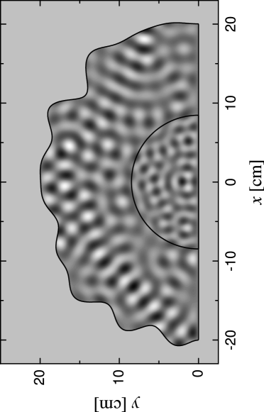
Figure 3: The reconstructed wave function $\Psi_{415}(r,\theta)$ of the chaotic half-circular microwave rough billiard. The amplitudes have been converted into a grey scale with white corresponding to large positive and black corresponding to large negative values, respectively. Dimensions of the billiard are given in cm. The position of the half-circular Teflon insert of radius $R_{d}=8.465$ cm is marked with a solid line.

Using the method of the “trial wave function” we were able to reconstruct 30 experimental wave functions of the rough half-circular billiard with the level number $N$ between 215 and 415. The wave functions were reconstructed on points of a square grid of side $4.2\cdot 10^{-4}$ m. As the quantitative measure of the sign assignment quality we chose the integral $\gamma\int_{\Gamma}|\Psi_{N}(r,\theta)|^{2}dl$ calculated along the billiard’s rough boundary $\Gamma$, where $\gamma$ is length of $\Gamma$. In Fig. 2 (b) we show the “trial wave function” $\Psi_{415}(R_{c},\theta)$ with the correctly assigned signs, which was used in the reconstruction of the wave function $\Psi_{415}(r,\theta)$ of the billiard (see Fig. 3). It is worth noting that inside of the Teflon insert the size of nodal domains are much smaller than outside of it. The remaining wave functions from the range $N=215-415$ were not reconstructed because of the accidental near-degeneration of the neighboring states or due to the problems with the measurements of $|\Psi_{N}(R_{c},\theta)|^{2}$ along a half-circle coinciding for its significant part with one or several of the nodal lines of $\Psi_{N}(r,\theta)$. The problem of the near-degenerated states is important because in the presence of the perturber the resonances are shifted, which may cause the initially non-overlapping states to become near-degenerated at certain positions of the perturber. Such a situation prevents us from the reconstruction of the wave functions. The problems mentioned are getting much more severe for $N>200$. Furthermore, the computation time $t_{r}$ required for reconstruction of the ”trial wave function” scales like $t_{r}\propto 2^{n_{z}-2}$, where $n_{z}$ is the number of identified zeros in the measured function $|\Psi_{N}(R_{c},\theta)|$.

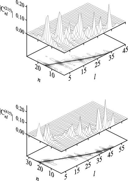
Figure 4: Structure of the energy surface in the regime of Shnirelman ergodicity. Here we show the moduli of amplitudes $|C^{(N)}_{nl}|$ for the wave functions: (a) $N=215$, (b) $N=415$. The wave functions are delocalized in the $n,l$ basis. Full lines show the energy surface (see text).

The structure of the energy surface Frahm97 of the billiard’s wave functions plays an important role in the identification of their ergodicity. To check it we extracted wave function amplitudes $C^{(N)}_{nl}=\left<n,l|N\right>$ in the basis $n,l$ of a half-circular ray-splitting billiard (desymmetrized annular ray-splitting billiard) Kohler1998 with radius $r_{max}$ and a half-circular Teflon insert of radius $R_{d}$ . The normalized eigenfunctions of the half-circular ray-splitting billiard are given by

$$\Phi_{nl}(r,\theta)=\left\{\begin{array}[]{cc}A_{ln}J_{l}(\eta\kappa_{ln}r)\sin(l\theta),&0\leq r\leq R_{d},\\ A_{ln}\left[C_{ln}J_{l}(\kappa_{ln}r)+D_{ln}Y_{l}(\kappa_{ln}r)\right]\sin(l\theta),&R_{d}\leq r\leq r_{max},\end{array}\right.$$

where $A_{ln}=\left\{\frac{\pi}{2}\left(\int_{0}^{R_{d}}rJ_{l}(\eta\kappa_{ln}r)^{2}dr+\int_{R_{d}}^{r_{max}}r\left[C_{ln}J_{l}(\kappa_{ln}r)+D_{ln}Y_{l}(\kappa_{ln}r)\right]^{2}dr\right)\right\}^{-\frac{1}{2}}$. $J_{l}(\kappa_{ln}r)$ and $Y_{l}(\kappa_{ln}r)$ are Bessel and Neumann functions, respectively. The main quantum number $n=1,2,3\ldots$ enumerates the zeros $y_{ln}=\kappa_{ln}r_{max}$ of the radial function

$$C_{ln}J_{l}(y_{ln})+D_{ln}Y_{l}(y_{ln})=0,$$

and $l=1,2,3\ldots$ is the angular momentum quantum number. The coefficients $C_{ln}$ and $D_{ln}$ can be determined from the continuity conditions of the wave function $\Phi_{nl}(r,\theta)$ and it’s derivative $\Phi_{nl}^{{}^{\prime}}(r,\theta)$ on Teflon’s boundary $R_{d}$

$$\left\{\begin{array}[]{cc}J_{l}(\eta\kappa_{ln}R_{d})=C_{ln}J_{l}(\kappa_{ln}R_{d})+D_{ln}Y_{l}(\kappa_{ln}R_{d}),\\ \eta J_{l}^{{}^{\prime}}(\eta\kappa_{ln}R_{d})=C_{ln}J_{l}^{{}^{\prime}}(\kappa_{ln}R_{d})+D_{ln}Y_{l}^{{}^{\prime}}(\kappa_{ln}R_{d}).\end{array}\right.$$

The moduli of amplitudes $|C^{(N)}_{nl}|$ and their projections into the energy surface for the representative experimental wave functions $N=215$ and $N=415$ are shown in Fig. 4. As expected, in the regime of Shnirelman ergodicity the wave functions are extended over the whole energy surface Hlushchuk01 . The full lines on the projection planes in Fig. 4(a) and Fig. 4(b) mark the energy surface of a half-circular annular ray-splitting billiard $H(n,l)\simeq E_{N}=k^{2}_{N}$ estimated from the formula $|H(n,l)-E_{N}|/E_{N}\leq 0.12$. The peaks $|C^{(N)}_{nl}|$ are spread almost perfectly along the lines marking the energy surface.

Figure 5: Panel (a): The amplitude distribution $P(\Psi_{N}A^{1/2})$ for the wave function $N=215$. Panel (b): The distribution $P(\Psi_{N}A^{1/2})$ for the wave function $N=415$. The amplitude distributions were constructed as histograms with bin equal to 0.2. The width of the distribution $P(\Psi)$ was rescaled to unity by multiplying normalized to unity wave function by the factor $A^{1/2}$, where $A$ denotes billiard’s area. Full lines show standard normalized Gaussian prediction $P_{0}(\Psi A^{1/2})=(1/\sqrt{2\pi})e^{-\Psi^{2}A/2}$.

Ergodic behavior of the measured wave functions can be also tested by evaluation of the amplitude distribution $P(\Psi_{N})$ Berry77 ; Kaufman88 . For irregular, chaotic states the probability of finding the value $\Psi_{N}$ at any point inside the billiard should be distributed as a Gaussian, $P(\Psi_{N})\sim e^{-\beta\Psi_{N}^{2}}$. In Fig. 5(a) we show the amplitude distribution $P(\Psi_{N}A^{1/2})$ for the wave function $N=215$ while in Fig. 5(b) the distribution $P(\Psi_{N}A^{1/2})$ for the wave function $N=415$ is presented. The distributions were constructed as normalized to unity histograms with the bin equal to 0.2. The width of the amplitude distributions $P(\Psi_{N})$ was rescaled to unity by multiplying normalized to unity wave functions by the factor $A^{1/2}$, where $A$ denotes billiard’s area (see formula (23) in Kaufman88 ). For all measured wave functions lying in the regime of Shnirelman ergodicity the distributions of $P(\Psi_{N}A^{1/2})$ were in good agreement with the standard normalized Gaussian prediction $P_{0}(\Psi A^{1/2})=(1/\sqrt{2\pi})e^{-\Psi^{2}A/2}$.

Figure 6: The number of nodal domains $\aleph_{N}$ (full circles) for the chaotic half-circular microwave ray-splitting rough billiard. Full line shows the least squares fit $\aleph_{N}=a_{1}N+b_{1}\sqrt{N}$ to the experimental data (see text), where $a_{1}=0.063\pm 0.023$, $b_{1}=0.77\pm 0.40$. The prediction of the theory of Bogomolny and Schmit Bogomolny2002 $a_{1}=0.062$.

The number of nodal domains $\aleph_{N}$ vs. the level number $N$ in the chaotic microwave ray-splitting rough billiard is plotted in Fig. 6. The full line in Fig. 6 shows the least squares fit $\aleph_{N}=a_{1}N+b_{1}\sqrt{N}$ of the experimental data, where $a_{1}=0.063\pm 0.023$, $b_{1}=0.77\pm 0.40$. The coefficient $a_{1}=0.063\pm 0.023$ coincides with the prediction of the percolation model of Bogomolny and Schmit Bogomolny2002 $\aleph_{N}/N\simeq 0.062$ within the error limits. The errors of the coefficients $a_{1}$ and $b_{1}$ are relatively high because the number of nodal domains fluctuates significantly in the function of the level number $N$, what was also demonstrated in Blum2002 (see Fig .(5)). It is worth mention that in the paper Savytskyy2004 the coefficient $a_{1}$ was estimated in the experiment with the microwave rough billiard without the ray-splitting Teflon insert. Its value $a_{1}=0.058\pm 0.006$ was also close to the theoretical prediction. The second term in the least squares fit corresponds to a contribution of boundary domains, i.e. domains that include the billiard boundary. Numerical calculations of Blum et al. Blum2002 performed for the Sinai and stadium billiards showed that the number of boundary domains scales as the number of the boundary intersections, that is as $\sqrt{N}$. Present results together with the results of Savytskyy2004 clearly suggest that in the rough billiards (with and without ray-splitting), at low level number $N$, the boundary domains also significantly influence the scaling of the number of nodal domains $\aleph_{N}$, leading to the departure from the predicted scaling $\aleph_{N}\sim N$.

Figure 7: The variance of the mean number of nodal domains divided by the level number $\sigma^{2}_{N}/N$ for the chaotic half-circular microwave ray-splitting rough billiard. Full line shows predicted by the theory limit $\sigma^{2}_{N}/N\simeq 0.05$, Bogomolny and Schmit Bogomolny2002 .

Measured wave functions of the ray-splitting billiard may be also used for the calculations of the variance $\sigma^{2}_{N}$ of the mean number of nodal domains. It was predicted in Bogomolny2002 that for chaotic wave functions the variance of the mean number of nodal domains should converge to the theoretical limit $\sigma^{2}_{N}\simeq 0.05N$. In Fig. 7 the variance of the mean number of nodal domains divided by the level number $\sigma^{2}_{N}/N$ is shown for the microwave ray-splitting rough billiard. The variance $\sigma^{2}_{N}=\frac{1}{N_{w}-1}\sum_{i=1}^{N_{w}}(\aleph_{N_{i}}-\langle\aleph_{N}\rangle)^{2}$ was calculated in the window of $N_{w}=5$ consecutive eigenstates measured between $215\leq N\leq 415$, where the mean number of nodal domains was defined as $\langle\aleph_{N}\rangle=\frac{1}{N_{w}}\sum_{i=1}^{N_{w}}\aleph_{N_{i}}$. For level numbers $N<300$ the variance $\sigma^{2}_{N}/N$ is above the predicted theoretical limit, however, for $300<N\leq 415$ it is slightly below it. A similar erratic behavior of $\sigma^{2}_{N}/N$ was also observed in Bogomolny2002 .

Figure 8: Distribution of nodal domain areas. Full line shows the prediction of percolation theory $\log_{10}(\langle n_{s}/n\rangle)=-\frac{187}{91}\log_{10}(\langle s/s_{min}\rangle)$. The least squares fit $\log_{10}(\langle n_{s}/n\rangle)=a_{2}-\tau\log_{10}(\langle s/s_{min}\rangle)$ of the experimental results lying within the vertical lines yields the scaling exponent $\tau=2.14\pm 0.12$ and $a_{2}=-0.06\pm 0.12$. The result of the fit is shown by the dashed line.

The percolation model Bogomolny2002 allows for applying the results of percolation theory to the description of nodal domains of chaotic billiards. The percolation theory predicts that the distribution of the areas $s$ of nodal clusters should obey the scaling behavior: $n_{s}\propto s^{-\tau}$. The scaling exponent Ziff1986 is found to be $\tau=187/91$. In Fig. 8 we present in logarithmic scales nodal domain areas distribution $\langle n_{s}/n\rangle$ vs. $\langle s/s_{min}\rangle$ obtained for the microwave ray-splitting rough billiard. The distribution $\langle n_{s}/n\rangle$ was constructed as normalized to unity histogram with the bin equal to 1. The areas $s$ of nodal domains were calculated by summing up the areas of the nearest neighboring grid sites having the same sign of the wave function. In Fig. 8 the vertical axis $\langle n_{s}/n\rangle=\frac{1}{N_{T}}\sum_{i=1}^{N_{T}}n_{s}^{(N)}/n^{(N)}$ represents the number of nodal domains $n_{s}^{(N)}$ of size $s$ divided by the total number of domains $n^{(N)}$ averaged over $N_{T}=30$ wave functions measured in the range $215\leq N\leq 415$. In these calculations we took into account only the nodal domains which entirely lied outside or inside of the Teflon insert for which percolation theory Ziff1986 should be applicable. The horizontal axis in Fig. 8 is expressed in the units of the smallest possible area $s_{min}^{(N)}$ Bogomolny2002 , $\langle s/s_{min}\rangle=\frac{1}{N_{T}}\sum_{i=1}^{N_{T}}s/s_{min}^{(N)}$, where $s_{min}^{(N)}=\pi(j_{01}/\eta k_{N})^{2}$ and $j_{01}\simeq 2.4048$ is the first zero of the Bessel function $J_{0}(j_{01})=0$. For nodal domains lying inside the Teflon insert the refraction index was according to our measurements $\eta=1.425$ while outside of the insert we assumed $\eta=1$. The full line in Fig. 8 shows the prediction of percolation theory $\log_{10}(\langle n_{s}/n\rangle)=-\frac{187}{91}\log_{10}(\langle s/s_{min}\rangle)$. In a broad range of $\log_{10}(\langle s/s_{min}\rangle)$, approximately from 0.2 to 1.4, which is marked by the two vertical lines the experimental results follow closely the theoretical prediction. The least squares fit $\log_{10}(\langle n_{s}/n\rangle)=a_{2}-\tau\log_{10}(\langle s/s_{min}\rangle)$ of the experimental results lying within the vertical lines gives the scaling exponent $\tau=2.14\pm 0.12$ and $a_{2}=-0.06\pm 0.12$, which is in a good agreement with the predicted $\tau=187/91\simeq 2.05$. The result of the fit is shown in Fig. 8 by the dashed line.

In summary, for the first time we measured high-lying wave functions of the chaotic microwave ray-splitting rough billiard. We showed that in the limit $N\rightarrow\infty$ the least squares fit of the experimental data reveals the asymptotic number of nodal domains $\aleph_{N}/N\simeq 0.063\pm 0.023$ that is close to the theoretical prediction $\aleph_{N}/N\simeq 0.062$ Bogomolny2002 . We demonstrate that for higher level numbers $N\simeq 215-415$ the variance of the mean number of nodal domains $\sigma^{2}/N$ is scattered around the theoretical limit $\sigma^{2}/N\simeq 0.05$. Following the results of percolationlike model proposed by Bogomolny2002 we confirmed that the distribution of the areas $s$ of nodal domains has power behavior $n_{s}\propto s^{-\tau}$, where scaling exponent is equal to $\tau=2.14\pm 0.12$. This result is in a good agreement with the prediction of percolation theory Ziff1986 , which predicts $\tau=187/91\simeq 2.05$. The experimental results presented in this paper strongly suggest that many properties of nodal domains in chaotic ray-splitting billiards are the same, like in conventional chaotic billiards without ray-splitting.

Acknowledgments. This work was supported by Ministry of Science and Information Society Technologies grant No. 2 P03B 047 24.

References

- (1) E. Bogomolny and C. Schmit, Phys. Rev. Lett. 88, 114102-1 (2002).
- (2) G. Blum, S. Gnutzmann, and U. Smilansky, Phys. Rev. Lett. 88, 114101-1 (2002).
- (3) N. Savytskyy, O. Hul, and L. Sirko Phys. Rev. E 70, 056209 (2004).
- (4) R. Blümel, T. M. Antonsen, B. Georgeot, E. Ott, and R. E. Prange, Phys. Rev. Lett. 76, 2476 (1996); Phys. Rev. E 53, 3284 (1996).
- (5) L. Sirko, P. M. Koch and R. Blümel, Phys. Rev. Lett. 78, 2940 (1997).
- (6) R. Blümel, P.M. Koch, and L. Sirko, Found. Phys. 31, 269 (2001).
- (7) L. Couchman, E. Ott, and T. M. Antonsen, Jr., Phys. Rev. A 46, 6193 (1992).
- (8) N. Savytskyy, A. Kohler, Sz. Bauch, R. Bl mel, and L. Sirko Phys. Rev. E 64, 036211 (2001).
- (9) Sz. Bauch, A. Błȩdowski, L. Sirko, P. M. Koch, and R. Blümel, Phys. Rev. E 57, 304 (1998).
- (10) Y. Hlushchuk, A. Kohler, Sz. Bauch, L. Sirko, R. Blümel, M. Barth, and H.-J. Stöckmann, Phys. Rev. E 61, 366 (2000).
- (11) R. Schäfer, U. Kuhl, M. Barth, and H.-J. Stöckmann, Found. Phys. 31, 475 (2001).
- (12) N. Savytskyy and L. Sirko, Phys. Rev. E 65, 066202-1 (2002).
- (13) Y. Hlushchuk, A. Błȩdowski, N. Savytskyy, and L. Sirko, Physica Scripta 64, 192 (2001).
- (14) Y. Hlushchuk, L. Sirko, U. Kuhl, M. Barth, H.-J. Stöckmann, Phys. Rev. E 63, 046208-1 (2001).
- (15) K.M. Frahm and D.L. Shepelyansky, Phys. Rev. Lett. 78, 1440 (1997).
- (16) K.M. Frahm and D.L. Shepelyansky, Phys. Rev. Lett. 79, 1833 (1997).
- (17) A. Shnirelman, Usp. Mat. Nauk. 29, N6, 18 (1974).
- (18) Y. Yamamoto and R.E. Sluster, Phys. Today 46(6), 66 (1993).
- (19) J.U. Nöckel and A.D. Stone, Nature 385, 45 (1997).
- (20) V. Doya, O. Legrand, and F. Mortessagne, Phys. Rev. Lett. 88, 014102 (2002).
- (21) Ya. M. Blanter, A.D. Mirlin, and B.A. Muzykantskii, Phys. Rev. Lett. 80, 4161 (1998).
- (22) L. Sirko, Sz. Bauch, Y. Hlushchuk, P.M. Koch, R. Blümel, M. Barth, U. Kuhl, and H.-J. Stöckmann, Phys. Lett. A 266, 331 (2000).
- (23) F. Borgonovi, Phys. Rev. Lett. 80, 4653 (1998).
- (24) L.C. Maier and J.C. Slater, J. Appl. Phys. 23, 68 (1952).
- (25) S. Sridhar, Phys. Rev. Lett. 67, 785 (1991).
- (26) C. Dembowski, H.-D. Gräf, A. Heine, R. Hofferbert, H. Rehfeld, and A. Richter, Phys. Rev. Lett. 84, 867 (2000).
- (27) D.H. Wu, J.S.A. Bridgewater, A. Gokirmak, and S.M. Anlage, Phys. Rev. Lett. 81, 2890 (1998).
- (28) A. Kohler and R. Blümel, Phys. Lett. A 238, 271 (1998).
- (29) J. Stein, H.-J. Stöckmann, and U. Stoffregen, Phys. Rev. Lett. 75, 53 (1995).
- (30) M. Hentschel and K. Richter, Phys. Rev. E 66, 056207 (2002).
- (31) S.W. McDonald and A.N. Kaufman, Phys. Rev A 37, 3067 (1988).
- (32) M.V. Berry, J. Phys. A 10, 2083 (1977).
- (33) R. M. Ziff, Phys. Rev. Lett. 56, 545 (1986).