DMPK Equation for the Edge Transport of Quantum Spin Hall Insulator

Abstract

Using the random matrix theory, we investigate the ensemble statistics of edge transport of a quantum spin Hall insulator with multiple edge states in the presence of quenched disorder. Dorokhov-Mello-Pereyra-Kumar equation applicable for such a system is established. It is found that a two-dimensional quantum spin Hall insulator is effectively a new type of one-dimensional (1D) quantum conductor with the different ensemble statistics from that of the ordinary 1D quantum conductor or the insulator with an even number of Kramers edge pairs. The ensemble statistics provides a physical manifestation of the $Z_{2}$-classification for the time-reversal invariant insulators.

One of the recent advances in condensed matter physics is the discovery of the quantum spin Hall insulator (QSHI) Kane and Mele (2005a); Bernevig et al. (2006). QSHI is a new type of topological insulator, which is gaped in the bulk, but has gapless edge modes that give rise to a quantized conductance. The key theoretical observation is the $Z_{2}$-classification for the time-reversal (TR) invariant insulating systems Kane and Mele (2005b): a two-dimensional (2D) insulator with an odd number of Kramers pairs of edge states and that with an even number are topologically distinct, and the QSHI has an odd number of Kramers pairs at its edge. Such a classification has been established by the analyses on the topological structure of the Bloch bands Kane and Mele (2005b); Moore and Balents (2007), and its robustness against the imperfections, such as the electron-electron interaction Wu et al. (2006) and disorders Xu and Moore (2006); Obuse et al. (2007, 2008), has also been discussed. Experimentally, a quantized conductance is observed in HgTe quantum wells, and is taken as the signature of the QSHI phase Konig et al. (2007), albeit not conclusively. Other experimental techniques, such as ARPES, are also employed for searching the new QSHIs Hsieh et al. (2008). At present, it is highly desirable to have more associations between the abstract $Z_{2}$-classification and the physically measurable properties.

In this Rapid Communication, we investigate the ensemble statistics of the edge transport of QSHI in the presence of quenched disorder. In essence, a two-dimensional (2D) QSHI is effectively a one-dimensional (1D) quantum conductor with an odd number of Kramers pairs of conducting channels. Such a 1D quantum conductor is actually a new species that can only be realized at the edge of a 2D QSHI Wu et al. (2006), different from the ordinary 1D conductors which always have an even number of Kramers pairs of conducting channels. We establish the Dorokhov-Mello-Pereyra-Kumar (DMPK) equation Beenakker (1997) applicable for such a system, upon which the ensemble statistics of the edge transport of the QSHI is investigated. The distinct ensemble statistics of the edge transport of the QSHI presents a physical manifestation of the $Z_{2}$-classification, and could be a useful probe for identifying the new TR invariant topological insulators.

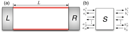
Figure 1: (color online) (a) The geometry of the system: an insulator with multiple edge conducting channels (represented by the color shaded bands at the two edges) is connected to the left and right measurement leads. (b) The transport along each of edges can be characterized by a $S$-matrix. $a_{i}^{+}$ ($b_{i}^{+}$) and $a_{i}^{-}$ ($b_{i}^{-}$) denote the right-going and left-going wave amplitudes, respectively. $a_{i}^{\pm}$ (or $b_{i}^{\pm}$) with the same index $i$ are related by the TR and form a Kramers pair. $N$ denotes the total number of Kramers pairs at each edge, and can be odd (QSHI) or even (ordinary insulator).

We consider a configuration shown in Fig. 1(a). Because the insulating bulk prevents the direct communication between the two edges, the system can be considered effectively as two independent 1D quantum conductors arranged in parallel. Each 1D conductor has $N$ Kramers pairs of conducting channels. We assume that the spin-orbit coupling is present, so the spins are not conserved in general. We do not assume the origin of the edge modes: they can be a result of the topological structure of the bulk bands, or from the extrinsic origins such as the surface dangling bonds.

In general, the transmission along the 1D conductor can be characterized by a $2N\times 2N$ $S$-matrix, which relates the incoming ($\psi_{\mathrm{in}}$) and outgoing ($\psi_{\mathrm{out}}$) wave amplitudes:

$$\psi_{\mathrm{out}}=S\psi_{\mathrm{in}}$$ (1)

where $\psi_{\mathrm{in}}\equiv(a_{1}^{+},a_{2}^{+}\dots a_{N}^{+};b_{1}^{-},b_{2}^{-}\dots b_{N}^{-})^{T}$ and $\psi_{\mathrm{out}}\equiv(a_{1}^{-},a_{2}^{-}\dots a_{N}^{-};b_{1}^{+},b_{2}^{+}\dots b_{N}^{+})^{T}$ (see Fig. 1(b)). In our labeling of the channel numbers, TR symmetry imposes the constraint on the $S$-matrix Bardarson (2008):

$$S^{T}=-S,$$ (2)

Moreover, the current conserving implies $S$-matrix must be unitary: $S^{\dagger}S=I$.

Under these constraints, the polar decomposition of the $S$-matrix reads Beenakker (1997); Bardarson (2008):

$$S=\left[\begin{array}[]{cc}U^{T}&0\\ 0&V^{T}\end{array}\right]\left[\begin{array}[]{cc}\Sigma&\mathcal{T}\\ -\mathcal{T}&-\Sigma\end{array}\right]\left[\begin{array}[]{cc}U&0\\ 0&V\end{array}\right]$$ (3)

where $U$ and $V$ are $N\times N$ unitary matrices, $\Sigma$ is a block diagonal matrix $\Sigma\equiv\Sigma_{1}\oplus\Sigma_{2}\oplus\cdots\oplus\Sigma_{n}(\oplus\bm{0}_{1\times 1})$ with $\Sigma_{i}=\sqrt{1-T_{i}}\left[\begin{array}[]{cc}0&1\\ -1&0\end{array}\right]$, and $\mathcal{T}=\mathrm{diag}[\sqrt{T_{1}},\sqrt{T_{1}},\sqrt{T_{2}},\sqrt{T_{2}}\cdots\sqrt{T_{n}},\sqrt{T_{n}}(,1)]$, for the even $N\equiv 2n$ (odd $N\equiv 2n+1$), $T_{i}$ denotes the $i$th transmission eigenvalue. One immediately sees that for the odd $N$, there is always one conducting channel that has the perfect transmission, without being adversely affected by the disorder. This is the reason behind the robust edge transport of QSHI.

The different ensemble statistics for the 1D conductors with the odd and the even $N$ can already be observed if we compute the volume element of the configuration space expanded by the independent parameters of the $S$-matrix: $\mathrm{d}\mu(S)=J_{0}\mathrm{d}\mu(U)\mathrm{d}\mu(V)\prod_{i}\mathrm{d}T_{i}$. To get the invariant measure $J_{0}$, we calculate $\mathrm{d}s^{2}=\mathrm{Tr}[\mathrm{d}S^{\dagger}\mathrm{d}S]\equiv g_{ij}\mathrm{d}x_{i}\mathrm{d}x_{j}$, and $J_{0}=\sqrt{\mathrm{det}[g_{ij}]}$, where $x\equiv\{U_{ij},V_{ij},T_{i}\}$ Mello et al. (1988). We obtain:

$$J_{0}=\prod_{i<j=1}^{n}(T_{i}-T_{j})^{4}\begin{cases}\prod_{i=1}^{n}T_{i},&\mathrm{even\,}N\\ \prod_{i=1}^{n}T_{i}(1-T_{i})^{2},&\mathrm{odd\,}N\end{cases}.$$ (4)

To determine the ensemble statistics of the 1D conductor, we derive the Dorokhov-Mello-Pereyra-Kumar (DMPK) equation for evolution of the joint probability distribution function of the transmission eigenvalues about the length $L$: $P(T_{1},T_{2}\cdots T_{n};L)$ Beenakker (1997). Basically, we consider a 1D quantum conductor of length $L$, and compute the change of the transmission eigenvalues upon attachment of a thin slice of length $\delta L$. Using the perturbation approach, we obtain Mello et al. (1988); Beenakker (1997):

$$\frac{1}{\delta s}\left\langle\delta T_{i}\right\rangle =-T_{i}+\frac{2n}{N(N-1)}T_{i}$$

$$\times\left(1-T_{i}+2\sum_{i\neq j}\frac{T_{i}+T_{j}-2T_{i}T_{j}}{T_{i}-T_{j}}\right),$$ (5)

$$\frac{1}{\delta s}\left\langle\delta T_{i}\delta T_{j}\right\rangle =\frac{4n}{N(N-1)}T_{i}^{2}\left(1-T_{i}\right)\delta_{ij},$$ (6)

where $\delta s\equiv\delta L/l$, $l$ is the mean free path defined by the first moment of the transmission eigenvalues of the thin slice: $\delta L/l=1-\left\langle\sum_{i=1}^{n}T_{i}(\delta L)\right\rangle/n$. The third and higher moments vanish at the first order of $\delta s$. DMPK equation is just the Fokker-Planker equation for the evolution of the distribution function $P$:

$$\frac{\partial P_{\lambda}}{\partial s}=\frac{2}{\gamma_{N}}\sum_{i=1}^{n}\frac{\partial}{\partial\lambda_{i}}\left\{\lambda_{i}(1+\lambda_{i})J\frac{\partial}{\partial\lambda_{i}}\left(\frac{P_{\lambda}}{J}\right)\right\},$$ (7)

where $\gamma_{N}\equiv N(N-1)/n$, and we have re-expressed the distribution function in a new set of variables $\lambda_{i}\equiv(1-T_{i})/T_{i}$, $P_{\lambda}(\lambda_{1},\lambda_{2}\cdots\lambda_{n},s)\equiv P(T_{1},T_{2},\cdots T_{n},L)\prod_{i=1}^{n}(1+\lambda_{i})^{-2}$, and

$$J=\prod_{i<j=1}^{n}(\lambda_{i}-\lambda_{j})^{4}\times\begin{cases}1,&\mbox{even}\,N\\ \prod_{i=1}^{n}\lambda_{i}^{2},&\mbox{odd}\,N\end{cases},$$ (8)

which actually coincides with Eq. (4) except for an unimportant denominator. We note that a similar DMPK equation was derived by Takane for the metallic carbon nanotubes Takane (2004).

Equations (7–8) are the central result of this paper. The equation is reduced to the usual DMPK equation of the ordinary 1D conductor of the symplectic ensemble ($\beta=4$) for the even $N\equiv 2n$ Beenakker (1997). On the other hand, for the odd $N\equiv 2n+1$, the equation is modified, and one expects a different distribution of the transmission eigenvalues. We will spell out its implications in the following.

Equation (7) turns out to be completely integrable for both even Caselle (1995) and odd $N$. To see this, we adopt a new set of variables $\{x_{i}\}$ that are related to $\{\lambda_{i}\}$ by $\lambda_{i}=\sinh^{2}x_{i}$, and $P_{x}(\{x_{i}\},s)\equiv P_{\lambda}\prod_{i=1}^{n}\sinh 2x_{i}$. We further make the substitution $P_{x}=\xi^{2}(x)\Psi(x,s)$, with

$$\xi(x)=\prod_{i<j=1}^{n}\sinh^{2}(x_{i}+x_{j})\sinh^{2}(x_{j}-x_{j})\\ \times\prod_{i=1}^{n}\sinh^{1/2}2x_{i}\begin{cases}1,&\mbox{even}\,N\\ \sinh^{2}x_{i}&\mbox{odd}\,N\end{cases},$$ (9)

and the equation is transformed to:

$$-\frac{\partial\Psi}{\partial s}=-\frac{1}{2\gamma_{N}}\left[\sum_{i=1}^{n}\frac{1}{\xi(x)^{2}}\frac{\partial}{\partial x_{i}}\xi(x)^{2}\frac{\partial}{\partial x_{i}}\right]\Psi.$$ (10)

We can then identify the operator inside the square bracket of the rhs. of Eq. (10) being the radial part of the Laplace-Beltrami operator for the irreducible symmetric space $\mathrm{SO}^{*}(2N)/U(N)$ Caselle (1995); Olshanetsky and Perelomov (1983). In particular, for the odd $N$, Equation (9) corresponds to a root system $BC_{n}$ of $\bm{\alpha}\equiv\{\pm\bm{e}_{i},\pm 2\bm{e}_{i},\pm\bm{e}_{i}\pm\bm{e}_{j}\}$, and has the appropriate multiplicity $m_{\bm{\alpha}}=\{4,1,4\}$ for a successful mapping to the Laplace-Beltrami operator (see Table B1 of Ref. Olshanetsky and Perelomov, 1983). This allows us to express the distribution function $P_{x}(x,s)$ as a superposition of the zonal spherical functions $\Phi_{k}(x)$ Caselle (1995):

$$P_{x}(\{x\},s)=C(s)\xi^{2}(x)\int\Phi_{k}(x)e^{-k^{2}s/2\gamma_{N}}\frac{\mathrm{d}^{n}k}{|c(k)|^{2}}.$$ (11)

For the odd $N$, the Gindikin-Karpelevich formula (Eq. (C12) of Ref. Olshanetsky and Perelomov, 1983) yields:

$$c(k)=\prod_{i<j=1}^{n}\frac{1}{g\left(\frac{k_{i}+k_{j}}{2}\right)g\left(\frac{k_{i}+k_{j}}{2}\right)}\\ \times\prod_{i=1}^{n}\frac{1}{(1+ik_{i})^{2}}\frac{\Gamma\left(i\frac{k_{i}}{2}\right)}{\Gamma\left(\frac{1}{2}+i\frac{k_{i}}{2}\right)},$$ (12)

where $g(x)\equiv\mathrm{i}x(1+\mathrm{i}x)$. The zonal spherical function $\Phi_{k}(x)$ can be constructed by a recurrent procedure (Eqs. (8.7-8.10) of Ref. Olshanetsky and Perelomov, 1983).

Using the asymptotic expansion of $\Phi_{k}(x)$ and following the same line of derivations as shown in Ref. Caselle, 1995, we can determine the asymptotic forms the distribution function. In the localization regime ($s\gg N$):

$$P_{x}(\{x_{i}\},s)\propto\prod_{i=1}^{n}\exp\left[-(\gamma_{N}/2s)(x_{i}-\bar{x}_{i})^{2}\right],$$ (13)

where $\bar{x}_{i}=(s/\gamma_{N})[3+4(i-1)]$. It follows that the average conductance $\sigma\sim 1+2\exp(-L/2\xi)$ with the localization length $\xi=Nl/2$ for the odd $N$, compared with $\xi=2(N-1)l$ for the ordinary 1D conductor (even $N$) Beenakker (1997). The conductance will have a log-normal distribution in this regime.

In the diffusive regime ($1\ll s\ll N$):

$$P_{x}(\{x_{i}\},s)\propto\prod_{i<j}\left(\sinh^{2}x_{i}-\sinh^{2}x_{j}\right)^{2}\left(x_{i}^{2}-x_{j}^{2}\right){}^{2}\\ \times\prod_{i}e^{-x_{i}^{2}\gamma_{N}/2s}\left(x_{i}\sinh 2x_{i}\right)^{1/2}(x_{i}\sinh x_{i})^{2}.$$ (14)

Compared with the ordinary 1D conductor Caselle (1995); Muttalib et al. (2005), the distribution function acquires an extra factor $\prod_{i}(x_{i}\sinh x_{i})^{2}$. Note that the correlations between the different transmission eigenvalues do not change.

We can determine the average and variance of the conductance in the regime $s\ll N$ using the method of moments of Mello and Stone Mello and Stone (1991); Beenakker (1997), which computes the moments of $M_{q}\equiv\sum_{i=1}^{n}T_{i}^{q}$ as expansion in inverse powers of $N$. From the DMPK equation (7), we can establish a chain of the coupled evolution equations for moments of $M_{q}$:

$$\frac{\gamma_{N}}{2}\frac{\partial\left\langle M_{q}^{p}\right\rangle}{\partial s}=2pq\sum_{k=1}^{q-1}\left\langle M_{q}^{p-1}M_{k}(M_{q-k}-M_{q-k+1})\right\rangle\\ -2pq\left\langle M_{q}^{p}M_{1}\right\rangle+pq^{2}\left\langle M_{q}^{p-1}M_{q+1}\right\rangle-pq\left[q\mp 1\right]\left\langle M_{q}^{p}\right\rangle\\ +p(p-1)q^{2}\left\langle M_{q}^{p-2}\left(M_{2q}-M_{2q+1}\right)\right\rangle,$$ (15)

where $\mp$ sign stands for the odd ($+$) and even ($-$) $N$, respectively. Since $M_{q}^{p}=\mathcal{O}(N^{p})$ in the particular regime, we can close the above equation order by order in the large $N$ limit. Noting that the average conductance $\sigma/\sigma_{0}=2\left\langle M_{1}\right\rangle+Z_{2}$ and the variance $\mathrm{var}(\sigma)/\sigma_{0}^{2}=4\left(\left\langle M_{1}^{2}\right\rangle-\left\langle M_{1}\right\rangle^{2}\right)$, $\sigma_{0}\equiv e^{2}/h$, we obtain:

$$\frac{\delta\sigma}{\sigma_{0}} =\frac{s^{3}}{3(1+s)^{3}}+Z_{2}\frac{s}{(1+s)^{2}}+\mathcal{O}\left(N^{-1}\right),$$ (16)

$$\frac{\mathrm{var}(\sigma)}{\sigma_{0}^{2}} =\frac{2}{15}\left[1-\frac{1+6s}{(1+s)^{6}}\right]+\mathcal{O}\left(N^{-1}\right),$$ (17)

where $\delta\sigma\equiv\sigma-N\sigma_{0}/(1+s)$ is the weak localization correction to the conductance, and we have introduced an index $Z_{2}$ that takes the value of $0$ (1) for the even (odd) $N$. Compared with the ordinary 1D conductor, the edge transport of QSHI will have a different weak localization correction but the same universal conductance fluctuation.

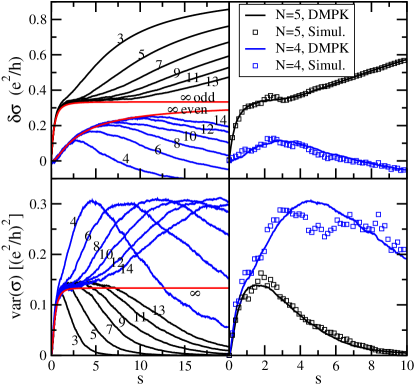
Figure 2: (color online) The weak localization correction to the conductance ($\delta\sigma$) and the variance of conductance ($\mathrm{var}(\sigma)$). Left: The results obtained from the numerical solutions of DMPK equation for different values of $N$ (the numbers by the curves). The $N\rightarrow\infty$ asymptotic behaviors Eqs. (16–17) are indicated by the red curves. Right: The comparison between the results from the DMPK equation and that from the simulation of the 2D model Eq. (18). The results for $N=4$ and $N=5$ are shown. In the 2D simulation, the parameters for the Kane-Mele model are: $t=1$, $\lambda_{\mathrm{so}}=0.2$, $\lambda_{R}=0.2$, $\lambda_{v}=0$ (see Ref. Kane and Mele, 2005b for the definitions of these parameters), and the other parameters are: $W=0.6$, $t_{1}=0.2$. The stripe has a width 48 lattice sites (LS) along the zig-zag direction. We have determined the mean free paths to be $l=2240$ LS ($N=4$) and $l=1680$ LS ($N=5$), respectively. 200 disorder configurations are averaged.

We have numerically solved the DMPK equation for different values of $N$, using a Monte-Carlo approach that simulates the diffusion of the transmission eigenvalues. The weak localization correction and the fluctuation of the conductance are calculated, shown in the left panel of Fig. 2. Equations (16)–(17) well predict the behaviors for both $\delta\sigma$ and $\mathrm{var}(\sigma)$ in the regime $s\ll N$. The difference between the odd $N$ and the even $N$ is evident. It is interesting to observe that although the variances of the conductance have the same asymptotic behaviors in the regime $s\ll N$ for the odd and even $N$ (see Eq. (17), they are very different in the crossover regime ($s\sim N$): $\mathrm{var}(\sigma)$ rapidly decreases to zero for the odd $N$, while it continues to increase and peaks at a value of $0.3(e^{2}/h)^{2}$ for the even $N$.

We further test our results against a real model of the 2D QSHI. We consider a system of a stack of $N$ layers of honeycomb lattice, each of which is described by the tight-binding Hamiltonian introduced by Kane and Mele Kane and Mele (2005b):

$$H=\sum_{l=1}^{N}H_{l}^{\mathrm{KM}}+\sum_{il}\epsilon_{il}c_{il}^{\dagger}c_{il}+t_{1}\sum_{\left\langle ll^{\prime}\right\rangle}c_{il}^{\dagger}c_{il^{\prime}},$$ (18)

where $c_{il}$ ($c_{il}^{\dagger}$) denotes the annihilation (creation) operator for lattice site $i$ at the $l$-th layer, $H_{l}^{\mathrm{KM}}$ denotes the Hamiltonian for the $l$th-layer and has the same form as Eq. (1) of Ref. Kane and Mele, 2005b, $\epsilon_{il}$ is the random site energy that uniformly distributes in $[-W/2,\,W/2]$, and the last term introduces the hopping between the neighboring layers with a hopping constant $t_{1}$. With the appropriate parameters, the system becomes an insulator with $N$-pairs of edge states. The presence of the Rashba spin-orbit coupling in $H^{\mathrm{KM}}$ and the disordered site energies will introduce backscattering between different edge channels. In the simulation, a small value of $W$ is chosen, so that the bulk is still insulating. This is different from the previous numerical investigations which concern more on the annihilation of the edge states by the strong disorder due to the breakdown of the bulk gap Onoda et al. (2007); Qiao et al. (2008). We have adopted an iterative approach based on the non-equilibrium Green’s function to calculate the conductance of a stripe of varying length Kazymyrenko and Waintal (2008). The results are presented in the right panel of Fig. 2. It is evident that both the weak localization correction to the conductance and the variance fit well with those predicted from the DMPK equation. It justifies our presumption that a 2D QSHI is effectively a 1D quantum conductor, and can be described by the DMPK equation (7–8).

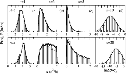
Figure 3: The distribution of conductance for $N=4$ (lower) and $5$ (upper). The drop lines shows the results from the DMPK equation. The solid lines indicates the distributions predicted by the asymptotic formulae Eq. (14) [(a)–(c)] and (13) [(d)]. $\Delta\sigma\equiv\sigma(s)-\sigma(\infty)$.

Figure 3 shows the distributions of conductance for different values of $s$. A crossover from the Gaussian distribution at the ballistic limit ($s=1$) to the log-normal distribution in the localization regime ($s=10,\,20$) can be observed. The difference between the odd and the even $N$ is the most notable in the crossover regime ($s=3,\,5$), where the distribution for $N=5$ shows a smooth high conductance tail, while that for $N=4$ has the a sharp threshold.

Finally, we discuss the possible experimental verification of our theoretical predictions. A 2D QSHI with the multiple pairs of edge states can be realized by confining the 3D QSHI in one direction Fu et al. (2007). An alternative and more flexible way is to put an ordinary mesoscopic 1D quantum wire in the proximity of the edge of a 2D QSHI sample, and couple them through a controllable gate. The ensemble statistics can then be measured for the combined system. By varying the coupling strength between the 1D wire and 2D QSHI, one expects a crossover of the ensemble statistics from the even $N$ to the odd $N$.

We thank C. Murdy for useful information. This work is supported by NSF of China (No. 10604063 and 10734110) and the National Basic Research Program of China (No. 2009CB929101 and 2006CB921304).

References

- Kane and Mele (2005a) C. L. Kane and E. J. Mele, Phys. Rev. Lett. 95, 226801 (2005a).
- Bernevig et al. (2006) B. A. Bernevig, T. L. Hughes, and S.-C. Zhang, Science 314, 1757 (2006).
- Kane and Mele (2005b) C. L. Kane and E. J. Mele, Phys. Rev. Lett. 95, 146802 (2005b).
- Moore and Balents (2007) J. E. Moore and L. Balents, Phys. Rev. B 75, 121306(R) (2007).
- Wu et al. (2006) C. Wu, B. A. Bernevig, and S.-C. Zhang, Phys. Rev. Lett. 96, 106401 (2006).
- Xu and Moore (2006) C. Xu and J. E. Moore, Phys. Rev. B 73, 045322 (2006).
- Obuse et al. (2007) H. Obuse, A. Furusaki, S. Ryu, and C. Mudry, Phys. Rev. B 76, 075301 (2007).
- Obuse et al. (2008) H. Obuse, A. Furusaki, S. Ryu, and C. Mudry, Phys. Rev. B 78, 115301 (2008).
- Konig et al. (2007) M. Konig, S. Wiedmann, C. Brune, A. Roth, H. Buhmann, L. W. Molenkamp, X.-L. Qi, and S.-C. Zhang, Science 318, 766 (2007).
- Hsieh et al. (2008) D. Hsieh, D. Qian, L. Wray, Y. Xia, Y. S. Hor, R. J. Cava, and M. Z. Hasan, Nature 452, 970 (2008).
- Beenakker (1997) C. W. J. Beenakker, Rev. Mod. Phys. 69, 731 (1997).
- Bardarson (2008) J. H. Bardarson, J. Phys. A 41, 405203 (2008).
- Mello et al. (1988) P. A. Mello, P. Pereyra, and N. Kumar, Ann. Phys. 181, 290 (1988).
- Takane (2004) Y. Takane, J. Phys. Soc. Jpn. 73, 9 (2004).
- Caselle (1995) M. Caselle, Phys. Rev. Lett. 74, 2776 (1995).
- Olshanetsky and Perelomov (1983) M. A. Olshanetsky and A. M. Perelomov, Phys. Rep. 94, 313 (1983).
- Muttalib et al. (2005) K. A. Muttalib, P. Markoš, and P. Wölfle, Phys. Rev. B 72, 125317 (2005).
- Mello and Stone (1991) P. A. Mello and A. D. Stone, Phys. Rev. B 44, 3559 (1991).
- Onoda et al. (2007) M. Onoda, Y. Avishai, and N. Nagaosa, Phys. Rev. Lett. 98, 076802 (2007).
- Qiao et al. (2008) Z. Qiao, J. Wang, Y. Wei, and H. Guo, Phys. Rev. Lett. 101, 016804 (2008).
- Kazymyrenko and Waintal (2008) K. Kazymyrenko and X. Waintal, Phys. Rev. B 77, 115119 (2008).
- Fu et al. (2007) L. Fu, C. L. Kane, and E. J. Mele, Phys. Rev. Lett. 98, 106803 (2007).