Tropical Atmospheric Circulations: Dynamic Stability and Transitions

Abstract.

In this article, we present a mathematical theory of the Walker circulation of the large-scale atmosphere over the tropics. This study leads to a new metastable state oscillation theory for the El Niño Southern Oscillation (ENSO), a typical inter-annual climate low frequency oscillation. The mathematical analysis is based on 1) the dynamic transition theory, 2) the geometric theory of incompressible flows, and 3) the scaling law for proper effect of the turbulent friction terms, developed recently by the authors.

1. Introduction

The atmosphere and ocean around the earth are rotating geophysical fluids, which are also two important components of the climate system. The phenomena of the atmosphere and ocean are extremely rich in their organization and complexity, involving a broad range of temporal and spatial scales. According to J. von Neumann [12], the motion of the atmosphere can be divided into three categories depending on the time scale of the prediction. They are motions corresponding respectively to the short time, medium range and long term behavior of the atmosphere. One of the primary goals in climate dynamics is to document, through careful theoretical and numerical studies, the presence of climate low frequency variability, to verify the robustness of this variability’s characteristics to changes in model parameters, and to help explain its physical mechanisms. The thorough understanding of this variability is a challenging problem with important practical implications for geophysical efforts to quantify predictability, analyze error growth in dynamical models, and develop efficient forecast methods. One typical source of the inter-annual climate low frequency variability is El Niño-Southern Oscillation (ENSO), which is associated with the Walker circulation of the atmosphere over the tropics. The main objective of this article is to introduce a mathematical theory of the general circulation of the atmosphere over the tropics.

The modeling part of the study is based on two important ingredients. First, from the general circulation point of view, there are three invariant regions of the atmosphere: the northern hemisphere, the southern hemisphere and the region over the tropics corresponding to zero latitude. The second is the new scaling law introduced recently by the authors, leading to correct circulation length scales.

The model is then analyzed using the dynamic transition theory and the geometric theory of incompressible flows, both developed recently by the authors. We refer the interested readers to [5] and the references therein for the geometric theory, and to the appendix, [4, 10] and the references therein for the dynamic transition theory. We mention in particular here that the main philosophy of the dynamic transition theory is to search for the full set of transition states, giving a complete characterization on stability and transition. This complete set of transition states represent the “physical reality” after the transition, and are described by a local attractor, rather than some steady states or periodic solutions or other type of orbits as part of this local attractor. With this theory, many longstanding phase transition problems are either solved or become more accessible leading to a number of physical predictions. For example, the study of phase transitions of helium-3 leads not only to a theoretical understanding of the phase transitions to superfluidity observed by experiments, but also to such physical predictions as the existence of a new superfluid phase C for liquid helium-3 [9].

The main results obtained in this article, on the one hand, verifies the general circulation patterns over the tropics associated with the Walker circulation, and, on the other hand, lead to a new mechanism of El Niño Southern Oscillation (ENSO), which will be published in an accompanying paper [8]. This new mechanism of the ENSO amounts to saying that ENSO, as a self-organizing and self-excitation system, with two highly coupled processes. The first is the oscillation between the two metastable warm (El Niño phase) and cold events (La Niña phase), and the second is the spatiotemporal oscillation of the sea surface temperature (SST) field. The interplay between these two processes gives rises the climate variability associated with the ENSO, leads to both the random and deterministic features of the ENSO, and defines a new natural feedback mechanism, which drives the sporadic oscillation of the ENSO.

The paper is organized as follows. In Section 2, we introduce the atmospheric circulation model over the tropics, which is analyzed in Sections 3 and 4, with concluding remarks given in Section 5.

2. Atmospheric Model over the Tropics

Physical laws governing the motion and states of the atmosphere and ocean can be described by the general equations of hydrodynamics and thermodynamics. As discussed in the Introduction, the atmospheric motion equations over the tropics are the Boussinesq equations restricted on $\theta=0$, where the meridional velocity component $u_{\theta}$ is set to zero, and the effect of the turbulent friction is taking into considering using the scaling law derived in [10]:

(2.1) $$\frac{\partial u_{\varphi}}{\partial t}=-(u\cdot\nabla)u_{\varphi}-\frac{u_{\varphi}u_{z}}{a}+\nu\left(\Delta u_{\varphi}+\frac{2}{a^{2}}\frac{\partial u_{z}}{\partial\varphi}-\frac{2u_{\varphi}}{a^{2}}\right)$$

$$\ \ \ \ -\sigma_{0}u_{\varphi}-2\Omega u_{z}-\frac{1}{\rho_{0}a}\frac{\partial p}{\partial\varphi},$$

$$\frac{\partial u_{z}}{\partial t}=-(u\cdot\nabla)u_{z}+\frac{u^{2}_{\varphi}}{a}+\nu\left(\Delta u_{z}-\frac{2}{a^{2}}\frac{\partial u_{\varphi}}{\partial\varphi}-\frac{2u_{z}}{a^{2}}\right)$$

$$\ \ \ \ -\sigma_{1}u_{z}+2\Omega u_{\varphi}-\frac{1}{\rho_{0}}\frac{\partial p}{\partial z}-(1-\alpha_{T}(T-T_{0}))g,$$

$$\frac{\partial T}{\partial t}=-(u\cdot\nabla)T+\kappa\Delta T+Q,$$

$$\frac{1}{a}\frac{\partial u_{\varphi}}{\partial\varphi}+\frac{\partial u_{z}}{\partial z}=0.$$

Here $\sigma_{i}=C_{i}h^{2}$ ($i=0,1$) represent the turbulent friction, $a$ is the radius of the earth, the space domain is taken as $M=S^{1}_{a}\times(a,a+h)$ with $S^{1}_{a}$ being the one-dimensional circle with radius $a$, and

$$(u\cdot\nabla)=\frac{u_{\varphi}}{a}\frac{\partial}{\partial\varphi}+u_{z}\frac{\partial}{\partial z},\qquad\Delta=\frac{1}{a^{2}}\frac{\partial^{2}}{\partial\varphi^{2}}+\frac{\partial^{2}}{\partial z^{2}}.$$

For simplicity, we denote

$$(x_{1},x_{2})=(a\varphi,z),\qquad(u_{1},u_{2})=(u_{\varphi},u_{z}).$$

In atmospheric physics, the temperature $T_{1}$ at the tropopause $z=a+h$ is a constant. We take $T_{0}$ as the average on the lower surface $z=a$. To make the nondimensional form, let

$$x=hx^{\prime},\qquad t=h^{2}t^{\prime}/\kappa,\qquad u=\kappa u^{\prime}/h,$$

$$T=(T_{0}-T_{1})T^{\prime}+T_{0}-(T-T_{0})x^{\prime}_{2},$$

$$p=\kappa\nu\rho_{0}p^{\prime}/h^{2}-g\rho_{0}(hx^{\prime}_{2}+\alpha_{T}(T_{0}-T_{1})hx^{\prime 2}/2).$$

Also, we define the Rayleigh number, the Prandtl number and the scaling laws by

(2.2) $$R=\frac{\alpha_{T}g(T_{0}-T_{1})h^{3}}{\kappa\nu},\qquad\text{\rm Pr }=\frac{\nu}{\kappa},\qquad\delta_{i}=C_{i}h^{4}/\nu\quad(i=0,1).$$

Omitting the primes, the nondimensional form of (2.1) reads

(2.3) $$\frac{\partial u_{1}}{\partial t}=\text{Pr }\left[\Delta u_{1}+\frac{2}{r_{0}}\frac{\partial u_{2}}{\partial x_{1}}-\frac{2}{r_{0}}u_{1}-\delta_{0}u_{1}-\frac{\partial p}{\partial x_{1}}\right]$$

$$\ \ \ \ -\omega u_{2}-(u\cdot\nabla)u_{1}-\frac{1}{r_{0}}u_{1}u_{2},$$

$$\frac{\partial u_{2}}{\partial t}=\text{Pr }\left[\Delta u_{2}-\frac{2}{r_{0}}\frac{\partial u_{1}}{\partial x_{1}}-\frac{2}{r_{0}}u_{2}-\delta_{1}u_{2}+RT-\frac{\partial p}{\partial x_{2}}\right]$$

$$\ \ \ \ +\omega u_{1}-(u\cdot\nabla)u_{2}-\frac{1}{r_{0}}u^{2}_{1},$$

$$\frac{\partial T}{\partial t}=\Delta T+u_{2}-(u\cdot\nabla)T+Q,$$

$$\frac{\partial u_{1}}{\partial x_{1}}+\frac{\partial u_{2}}{\partial x_{2}}=0,$$

where $(x_{1},x_{2})\in M=(0,2\pi r_{0})\times(r_{0},r_{0}+1)$, $\delta_{0}$ and $\delta_{1}$ are as in (2.2), $(u\cdot\nabla)$ and $\Delta$ as usual differential operators, and

(2.4) $$\omega=\frac{2\Omega h^{2}}{\kappa}.$$

The problem is supplemented with the natural periodic boundary condition in the $x_{1}$-direction, and the free-slip boundary condition on the top and bottom boundary:

(2.5) $$(u,T)(x_{1}+2\pi r_{0},x_{2},t)=(u,T)(x_{1},x_{2},t),$$

(2.6) $$\left\{\begin{aligned} &u_{2}=0,\ \frac{\partial u_{1}}{\partial x_{2}}=0,T=\varphi(x_{1})\qquad&&\text{at}\ x_{2}=r_{0},\\ &u_{2}=0,\ \frac{\partial u_{1}}{\partial x_{2}}=0,\ T=0\qquad&&\text{at}\ x_{2}=r_{0}+1.\end{aligned}\right.$$

Here $\varphi(x_{1})$ is the temperature deviation from the average $T_{0}$ on the equatorial surface and is periodic, i.e.,

$$\int^{2\pi r_{0}}_{0}\varphi(x_{1})dx_{1}=0\ \ \ \ \text{and }\ \varphi(x_{1})=\varphi(x_{1}+2\pi r_{0}).$$

The deviation $\varphi(x_{1})$ is mainly caused by a difference in the specific heat capacities between the sea water and land.

3. Walker Circulation under the Idealized Conditions

In an idealized case, the temperature deviation $\varphi$ vanishes. In this case, the study of transition of (2.3) is of special importance to understand the longitudinal circulation. Here, we are devoted to discuss the dynamic bifurcation of (2.3), the Walker cell structure of bifurcated solutions, and the convection scale under the idealized boundary condition

(3.1) $$\varphi(x_{1})=0 \text{ for any }0\leq x_{1}\leq 2\pi r_{0},$$

$$Q=0 \text{ in (\ref{10.39})}.$$

For the problem (2.3) with (2.5) and (2.6), let

$$H=\{(u,T)\in L^{2}(M)^{3}\ |\ \text{div}u=0,(u,T)\ \text{satisfies}\ (\ref{10.41}\},$$

$$H_{1}=\{(u,T)\in H^{2}(M)^{3}\cap H\ |\ (u,T)\ \text{satisfies\ one\ of}\ (\ref{10.41})\text{ and }(\ref{10.44})\}.$$

Then, define the operators $L_{R}=A+B_{R}$ and $G:H_{1}\rightarrow H$ by

(3.2) $$A\psi=P(P_{k}(\Delta u_{1}+\frac{2}{r_{0}}\frac{\partial u_{2}}{\partial x_{1}}-\delta^{\prime}_{0}u_{1}),\text{Pr }(\Delta u_{2}-\frac{2}{r_{0}}\frac{\partial u_{1}}{\partial x_{1}}-\delta^{\prime}_{1}u_{2}),\Delta T),$$

$$B_{R}\psi=P(-\omega u_{2},\omega u_{1}+\text{Pr }RT,u_{2}),$$

$$G\psi=P(((u\cdot\nabla)u_{1}+\frac{u_{1}u_{2}}{r_{0}}),((u\cdot\nabla)u_{2}-\frac{u^{2}_{1}}{r_{0}}),(u\cdot\nabla)T),$$

where $\psi=(u,T)\in H_{1}$, $P:L^{2}(M)^{3}\rightarrow H$ is the Leray Projection, and $\delta^{\prime}_{i}=\frac{2}{r^{2}_{0}}+\delta_{i}$ $(i=0,1)$. Under the definitions (3.2), the problem (2.3) with one of (2.5) and (2.6) is equivalent to the following abstract equation

(3.3) $$\frac{d\psi}{dt}=L_{R}\psi+G(\psi).$$

Consider the eigenvalue problem

(3.4) $$L_{R}\psi=\beta(R)\psi,$$

which is equivalent to

(3.5) $$\Delta u_{1}+\frac{2}{r_{0}}\frac{\partial u_{2}}{\partial x_{1}}-\delta^{\prime}_{0}u_{1}-P^{-1}_{r}\omega u_{1}-\frac{\partial p}{\partial x_{1}}=P^{-1}_{r}\beta u_{1},$$

$$\Delta u_{2}-\frac{2}{r_{0}}\frac{\partial u_{1}}{\partial x_{1}}-\delta^{\prime}_{1}u_{2}+P^{-1}_{r}\omega u_{2}+RT-\frac{\partial p}{\partial x_{2}}=P^{-1}_{r}\beta u_{2},$$

$$\Delta T+u_{2}=\beta T,$$

$$\text{div}u=0,$$

with the boundary conditions (2.5) and (2.6).

We shall see later that these equations (3.5) are symmetric, which implies, in particular, that all eigenvalues $\beta_{j}(R)$ are real, and there exists a number $R_{c}$, called the first critical Rayleigh number, such that

(3.6) $$\beta_{i}(R)\left\{\begin{aligned} &<0&&\text{ if }R<R_{c},\\ &=0&&\text{ if }R=R_{c},\\ &>0&&\text{ if }R>R_{c}\end{aligned}\right. \text{ for }i=1,2,$$

(3.7) $$\beta_{j}(R_{c})<0 \text{ for }j>2.$$

The following theorem provides a theoretical basis to understand the equatorial Walker circulation.

Theorem 3.1.

Under the idealized condition (3.1), the problem (2.3) with (2.5) and (2.6) undergoes a Type-I transition at the critical Rayleigh number $R=R_{c}$. More precisely, the following statements hold true:

• When the Rayleigh number $R\leq R_{c}$, the equilibrium solution $(u,T)=0$ is globally stable in the phase space $H$.

• When $R_{c}<R<R_{c}+\delta$ for some $\delta>0$, this problem bifurcates from $((u,T),R)=(0,R_{c})$ to an attractor ${\mathcal{A}}_{R}=S^{1}$, consisting of steady state solutions, which attracts $H\setminus\Gamma$ , where $\Gamma$ is the stable manifold of $(u,T)=0$ with codimension two.

• For each steady state solution $\psi_{R}=(u_{R},T_{R})\in{\mathcal{A}_{R}},u_{R}$ is topologically equivalent to the structure as shown in Figure 3.1.

• For any initial value $\psi_{0}=(u_{0},T_{0})\in H\setminus(\Gamma\cup E)$, there exists a time $t_{0}\geq 0$ such that for any $t>t_{0}$ the velocity field $u(t,\psi_{0})$ is topologically equivalent to the structure as shown in Figure 3.2 either (a) or (b), where $\psi=(u(t,\psi_{0}),T(t,\psi_{0}))$ is the solutions of the problem with $\psi(0)=\psi_{0}$, and

  $$E=\{(u,T)\in H|\ \int^{r_{0}+1}_{r_{0}}u_{1}dx_{2}=0\}.$$

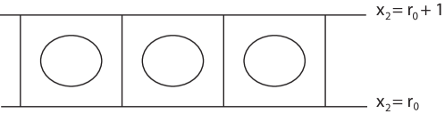
Figure 3.1. The cell structure of the steady state solutions in the bifurcated attractor ${\mathcal{A}}_{R}$.

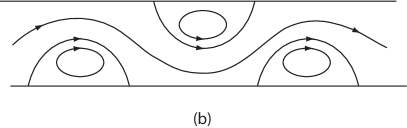
Figure 3.2. The Walker cell structure with the cells separated by a cross channel flow: (a) a westbound cross channel flow, and (b) an eastbound cross channel flow. This cross-channel flow pattern has the same topological structure as the Walker circulation over the tropics and the Branstator-Kushnir waves in the atmospheric dynamics [1, 2].

Proof of Theorem 3.1.

We proceed in the following several steps.

Step 1. We shows that equations (2.3) have an equivalent form as the classical 2D Bénard problem.

Since the velocity field $u$ defined on $M=S^{1}\times(r_{0},r_{0}+1)$ is divergence-free, there exists a stream function $\varphi$ such that

$$u_{1}=\frac{\partial\varphi}{\partial x_{2}},\ \ \ \ u_{2}=-\frac{\partial\varphi}{\partial x_{1}},$$

satisfying the given boundary conditions. Therefore, the following two vector fields

(3.8) $$(-\omega u_{2},\omega u_{1})=\omega\nabla\varphi,$$

$$(\frac{2}{r_{0}}\frac{\partial u_{2}}{\partial x_{1}},\frac{2}{r_{0}}\frac{\partial u_{1}}{\partial x_{1}})=-\frac{2}{r_{0}}\nabla\frac{\partial\varphi}{\partial x_{1}},$$

are gradient fields, which can be balanced by $\nabla p$ in (2.3). Hence, (2.3) are equivalent to

(3.9) $$\frac{\partial u_{1}}{\partial t}+(u\cdot\nabla)u_{1}+\frac{u_{1}u_{2}}{r_{0}}=\text{Pr }\left[\Delta u_{1}-\delta^{\prime}_{0}u_{1}-\frac{\partial p}{\partial x_{1}}\right],$$

$$\frac{\partial u_{2}}{\partial t}+(u\cdot\nabla)u_{2}-\frac{u^{2}_{1}}{r_{0}}=\text{Pr }\left[\Delta u_{2}-\delta^{\prime}_{1}u_{2}+RT-\frac{\partial p}{\partial x_{2}}\right],$$

$$\frac{\partial T}{\partial t}+(u\cdot\nabla)T=\Delta T+u_{2},$$

$$\text{div}u=0.$$

Therefore, equation (3.3) is also an abstract form of (3.9). Thus, equations (3.4) and (3.5) are symmetric. It is clear that the operator $G$ defined in (3.2) is orthogonal. Hence, the attractor bifurcation theorem for the Rayleigh-Bénard convection proved in [3] is also valid for the problem (2.3) with (2.5), (2.6). Thus, this transition of the problem is Type-I (i.e., continuous), and Assertion (1) is proved.

Step 2. Proof of Assertion (2). We only need to verify that the attractor ${\mathcal{A}}_{R}$ is homeomorphic to a circle, and consisting of singular points of (3.3). We consider the first eigenvectors of (3.5) at $R=R_{c}$. By (3.8), equations (3.5) at $R=R_{c}$ are equivalent to the form

(3.10) $$\Delta u_{1}-\delta^{\prime}_{0}u_{1}-\frac{\partial p}{\partial x_{1}}=0,$$

$$\Delta u_{2}-\delta^{\prime}_{1}u_{2}+R_{c}T-\frac{\partial p}{\partial x_{2}}=0,$$

$$\Delta T+u_{2}=0,$$

$$\text{div}u=0,$$

with the boundary conditions (2.5) and (2.6)

As in [3, 6], we see that the multiplicity of $R_{c}$ in (3.10) is $m=2$, and the corresponding eigenvectors are given by

(3.11) $$\psi_{1}=(u_{1},u_{2},T)=\left(-\sin\frac{kx_{1}}{r_{0}}H^{\prime}(x_{2}),\frac{k}{r_{0}}\cos\frac{kx_{1}}{r_{0}}H(x_{2}),\cos\frac{kx_{1}}{r_{0}}\Phi(x_{2})\right),$$

(3.12) $$\tilde{\psi}_{1}=\left(\tilde{u}_{1},\tilde{u}_{2},\tilde{T})=(\cos\frac{kx_{1}}{r_{0}}H^{\prime}(x_{2}),\frac{k}{r_{0}}\sin\frac{kx_{1}}{r_{0}}H(x_{2}),\sin\frac{kx_{1}}{r_{0}}\Phi(x_{2})\right),$$

where the functions $H(x_{2})$ and $\Phi(x_{2})$ satisfy that

(3.13) $$\left\{\begin{aligned} &(D^{4}-(\alpha^{2}+\alpha^{2}_{0})D^{2}+\alpha^{2}\alpha^{2}_{1})H=\alpha R_{c}\Phi,\\ &-(D^{2}-\alpha^{2})\Phi=\alpha H,\end{aligned}\right.$$

(3.14) $$H=H^{\prime\prime}=0,\ \ \ \ \Phi=0\qquad\text{ at }x_{2}=r_{0},r_{0}+1,$$

where $D=d/dx_{2},\alpha=k/r_{0},\alpha^{2}_{i}=\alpha^{2}+\delta^{\prime}_{i}$ $(i=0,1)$.

Since (3.13) with (3.14) are symmetric, we define a number $\alpha$ by

(3.15) $$\alpha=\frac{1}{\|\psi_{1}\|^{2}}<G(\Psi,\psi_{1})+G(\psi_{1},\Psi),\psi_{1}>,$$

where $\alpha$ is the number as in (A.6), and $\Psi$ is the center manifold function and by [4] it satisfies that

(3.16) $$-L_{R_{c}}\Psi=G(\psi_{1},\psi_{1})+\text{higher order terms},$$

and $L_{R}$ is defined by (3.2), and $G(\tilde{\psi},\psi)$ defined by

$$G(\tilde{\psi},\psi)=P\left((\tilde{u}\cdot\nabla)u_{1}+\frac{\tilde{u}_{1}u_{2}}{r_{0}},(\tilde{u}\cdot\nabla)u_{2}+\frac{\tilde{u}_{1}u_{1}}{r_{0}},(\tilde{u}\cdot\nabla)T\right),$$

for any $\tilde{\psi}=(\tilde{u},\tilde{T}),\psi=(u,T)\in H_{1}$. Obviously, for any $\psi,\tilde{\psi}\in H_{1}$, we have

$$<G(\tilde{\psi},\psi),\psi>=0,$$

$$<G(\psi,\tilde{\psi}),\psi>=-<G(\psi,\psi),\tilde{\psi}>.$$

Hence, we derive from (3.15) and (3.16) that

$$\alpha=-\frac{1}{\|\psi_{1}\|^{2}}<G(\psi_{1},\psi_{1}),\Psi>=-\frac{1}{\|\psi_{1}\|^{2}}<-L_{R_{c}}\Psi,\Psi>.$$

Due to (3.8), $-L_{R}$ is a symmetric sectorial operator. Thus, we have

$$\alpha=-\frac{1}{\|\psi_{1}\|^{2}}<(-L_{R_{c}})^{{1}/{2}}\Psi,(-L_{R_{c}})^{{1}/{2}}\Psi><0.$$

Then, as in [6], Assertion (2) follows.

Step 3. Proof of Assertion (3). By Step 1 and the attractor bifurcation theorem, each steady state solution $\varphi\in{\mathcal{A}}_{R}$ can be expressed as

(3.17) $$\varphi=|\beta_{1}(R)/\alpha|^{{1}/{2}}(x\psi_{1}+y\tilde{\psi}_{1})+o(\beta_{1}(R)),$$

where $\psi_{1},\tilde{\psi}_{1}$ are given by (3.11) and (3.12), $x^{2}+y^{2}=1$, and $\beta_{1}(R)$ is the first eigenvalue of (3.4) satisfying (3.6).

Let $\varphi=(e,T)$. Then, by (3.17) the velocity field $e$ is written as

$$e=\left\{\begin{aligned} &r(R)\cos\frac{k}{r_{0}}(x_{1}+\theta)H^{\prime}(x_{2})+o(r(R)),\\ &\frac{k}{r_{0}}r(R)\sin\frac{k}{r_{0}}(x_{1}+\theta)H(x_{2})+o(r(R)),\end{aligned}\right.$$

where $r(R)=|\beta_{1}(R)/\alpha|^{{1}/{2}},(x,y)=(\cos\theta,\sin\theta)$.

By (3.13) and (3.14), $H(x_{2})=\sin j\pi(x_{2}-r_{0}),j\in Z$. But, for the first eigenvectors $\psi_{1}$ and $\tilde{\psi}_{1}$, we have

$$H(x_{2})=\sin\pi(x_{2}-r_{0}).$$

Thus, $e$ is expressed as

(3.18) $$e=e_{0}+o(r(R)),$$

(3.19) $$e_{0}=\left\{\begin{aligned} &\pi r(R)\cos\frac{k}{r_{0}}(x_{1}+\theta)\cos\pi(x_{2}-r_{0}),\\ &\frac{k}{r_{0}}r(R)\sin\frac{k}{r_{0}}(x_{1}+\theta)\sin\pi(x_{2}-r_{0}),\end{aligned}\right.$$

It is easy to check that $e_{0}$ is regular, therefore $e$ is also regular as $R_{c}<R<R_{c}+\delta$ for some $\delta>0$. Obviously, the vector field $e_{0}$ is topologically equivalent to the structure as shown in Figure 3.1.

By the structural stability theorem in [5], the vector field $e_{0}$ in (3.19) is not structurally stable in $H_{1}$, because the boundary saddle points on $x_{2}=r_{0}$ are connected to saddle points on $x_{2}=r_{0}+1$, a different connected component. However, $e_{0}$ is structurally stable in the space

$$\tilde{H}=\{(u,T)\in H|\ \int^{2\pi r_{0}}_{0}\int^{r_{0}+1}_{r_{0}}udx=0\}.$$

To see this, we know that if $u\in\tilde{H}$, then $u=(u_{1},u_{2})\neq$constant, and $u_{1}$ has the Fourier expansion

$$u_{1}=\sum\limits_{k,j}(x_{kj}\cos\frac{kx_{1}}{r_{0}}+y_{kj}\sin\frac{kx_{1}}{r_{0}})\cos j\pi(x_{2}-r_{0}).$$

It follows that

(3.20) $$\int^{r_{0}+1}_{r_{0}}u_{1}dx_{2}=0\ \ \ \ \forall u=(u_{1},u_{2})\in\tilde{H}$$

According to the Connection Lemma (Lemma 2.3.1 in Ma and Wang [5]), from (3.20) one can infer that a vector field $u\in\tilde{H}$ is structurally stable if and only if $u$ is regular, and all interior saddle points of $u$ are self-connected. Therefore, $e_{0}$ is structurally stable in $\tilde{H}$.

If we can prove that the vector field $e$ given by (3.18) is in $\tilde{H}$, then, as $R_{c}<R<R_{c}+\delta$, $e$ is topologically equivalent to $e_{0}$. Hence, to prove Assertion (3), it suffices to verify that $e\in\tilde{H}$.

Obviously, $\tilde{H}$ is an invariant space for the operator $L_{R}+G$ defined by (3.2), and the orthogonal complementary $\tilde{H}^{\bot}$ of $\tilde{H}$ in $H$ is

$$\tilde{H}^{\bot}=\{(u,T)\in H|\ u=(c,0),T=0,c\in\mathbb{R}^{1}\}$$

It is readily to prove that all steady state solutions of (3.3) are in $\tilde{H}$. Thus, Assertion (3) is proved.

Step 4. Proof of Assertion (4). For any initial value $\psi_{0}=(u_{0},T_{0})\in H\setminus\tilde{H},\psi_{0}$ can be written as

$$\psi_{0}=c_{0}+\Phi_{0},\Phi_{0}\in\tilde{H},$$

$$c_{0}=(\alpha_{0},0,0)\in\tilde{H}^{\bot},\ \ \ \ \alpha_{0}\neq 0.$$

Since $G(\psi)\in\tilde{H},\forall\psi\in H$, the solution $\psi(t,\psi_{0})$ of (3.3) with $\psi(0,\psi_{0})=\psi_{0}$ must be in the form

$$\psi(t,\psi_{0})=C_{0}e^{-\delta^{\prime}_{0}t}+\Phi(t,\psi_{0}),\ \ \ \ \Phi\in\tilde{H}.$$

In addition, we know that for each $\psi_{0}\in H/\Gamma$ there is a steady state solution $\varphi=(e,T)\in{\mathcal{A}}_{R}$ such that

$$\lim\limits_{t\rightarrow\infty}\|\psi(t,\psi_{0})-\varphi\|_{C^{r}}=0\ \ \ \ \text{for\ any}\ r\geq 1.$$

Then, for any $\psi_{0}\in H\setminus(\tilde{H}\cup\Gamma)$, it follows that there exists a time $t_{0}>0$ such that the velocity field $u(t,\psi_{0})$ of $\psi(t_{0},\psi_{0})$ is topologically equivalent to the following vector field for any $t>t_{0}$

$$\tilde{u}=e+c_{0}e^{-\delta^{\prime}_{0}t}=e+(\alpha_{0}e^{-\delta^{\prime}_{0}t},0,0),$$

where $e$ is as in (3.18).

The vector field $e$ has the roll structure as shown in Figure 3.1, and $c_{0}e^{-\delta^{\prime}_{0}t}$ is a parallel channel flow. Hence, it is easy to show that $\tilde{u}=e+c_{0}e^{-\delta^{\prime}_{0}t}$ is topologically equivalent to the structure as shown in Figure 3.2 (a) as $\alpha_{0}<0$, and to the structure as shown in Figure 3.2 (b) as $\alpha_{0}>0$, for $t>t_{0}$ large. Assertion (4) is proved. ∎

4. Walker circulation under natural conditions

We now return the natural boundary condition

$$\varphi(x_{1})\not\equiv 0\quad\text{ and }\quad Q\not=0.$$

In this case, equations (2.3) admits a steady state solution

(4.1) $$\tilde{\psi}=(V,J),\ \ \ \ (V=(V_{1},V_{2})).$$

Consider the deviation from this basic state:

$$u\rightarrow u+V,\ \ \ \ T\rightarrow T+J.$$

Then (2.3) becomes

(4.2) $$\frac{\partial u_{1}}{\partial t}+(u\cdot\nabla)u_{1}+\frac{u_{1}u_{2}}{r_{0}}=\text{Pr }[\Delta u_{1}-\delta^{\prime}_{0}u_{1}-\frac{\partial p}{\partial x_{1}}]$$

$$\ \ \ \ -(u\cdot\nabla)u_{1}-(u\cdot\nabla)V_{1}-\frac{V_{1}}{r_{0}}u_{2}-\frac{V_{2}}{r_{0}}u_{1},$$

$$\frac{\partial u_{2}}{\partial t}+(u\cdot\nabla)u_{2}-\frac{u^{2}_{1}}{r_{0}}=\text{Pr }[\Delta u_{2}-\delta^{\prime}_{1}u_{2}+RT-\frac{\partial p}{\partial x_{2}}]$$

$$\ \ \ \ -(u\cdot\nabla)u_{2}-(u\cdot\nabla)V_{2}+\frac{2V_{1}}{r_{0}}u_{1},$$

$$\frac{\partial T}{\partial t}+(u\cdot\nabla)T=\Delta T+u_{2}-(u\cdot\nabla)J-(u\cdot\nabla)T,$$

$$\text{div}u=0.$$

The boundary conditions are the free-free boundary conditions given by

(4.3) $$(u,T)\ \text{is\ periodic\ in}\ x_{1}-\text{direction},$$

$$T=0,u_{2}=0,\frac{\partial u_{1}}{\partial x_{2}}=0\ \text{at}\ x_{2}=r_{0},r_{0}+1.$$

Let the operators $L_{R}=A+B_{R}$ and $G:H_{1}\rightarrow H$ be as in (3.2), and ${\mathcal{L}}^{\varepsilon}:H_{1}\rightarrow H$ be defined by

$${\mathcal{L}}^{\varepsilon}\psi = P(-(V\cdot\nabla)u_{1}-(u\cdot\nabla)V_{1}-\frac{V_{1}}{r_{0}}u_{2}-\frac{V_{2}}{r_{0}}u_{1},$$

$$-(V\cdot\nabla)u_{2}-(u\cdot\nabla)V_{2}+\frac{2V_{1}}{r_{0}}u_{1},-(u\cdot\nabla)J-(V\cdot\nabla)T).$$

Then, the problem (4.2) and (4.3) is equivalent to the abstract form

(4.4) $$\frac{d\psi}{dt}=L_{R}\psi+{\mathcal{L}}^{\varepsilon}\psi+G(\psi).$$

Consider the eigenvalue problem

(4.5) $$L_{R}\psi+{\mathcal{L}}^{\varepsilon}\psi=\beta^{\varepsilon}(R)\psi.$$

It is known that $|\varphi(x_{1})|$ and $Q\not=0$ are small, with $\Delta T=T_{0}-T_{1}\cong 100^{\circ}C$ as unit. Hence, the steady state solution $(V,J)$ is also small:

$$\|(V,J)\|_{L^{2}}=\varepsilon\ll 1.$$

Thus, (4.2) is a perturbation equation of (2.3).

Since perturbation terms involving $(V,J)$ are not invariant under the zonal translation (in the $x_{1}$-direction), for general small functions $\varphi(x_{1})\neq 0$, the first eigenvalues of (4.2) are (real or complex) simple, and by the perturbation theorems in [4], all eigenvalues of linearized equation of (4.2) satisfy the following principle of exchange of stability (PES):

$$\text{Re}\beta^{\varepsilon}_{i}(R)\left\{\begin{aligned} &<0&&\text{ for }R<R^{\varepsilon}_{c},\\ &=0&&\text{ for }R=R^{\varepsilon}_{c},\\ &>0&&\text{ for }R>R^{\varepsilon}_{c},\end{aligned}\right. \text{ for any }1\leq i\leq m,$$

$$\text{Re}\beta^{e}_{j}(R^{\varepsilon}_{c})<0 \text{ for any }j\geq m+1,$$

where $m=1$ as $\beta^{\varepsilon}_{1}(R)$ is real, $m=2$ as $\beta^{\varepsilon}_{1}(R)$ is complex near $R^{\varepsilon}_{c}$, and $R^{\varepsilon}_{c}$ is the critical Rayleigh number of perturbed system (4.2).

The following two theorems follow directly from Theorem 3.1 and the perturbation theorems in the appendix or in [4].

Theorem 4.1.

Let $\beta^{\varepsilon}_{1}(R)$ near $R=R^{\varepsilon}_{c}$ be a real eigenvalue. Then the system (4.2) has a transition at $R=R^{\varepsilon}_{c}$, which is either mixed (Type-III) or continuous (Type-I), depending on the temperature deviation $\varphi(x_{1})$. Moreover, we have the following assertions:

• If the transition is Type-I, then as $R^{\varepsilon}_{c}<R<R^{\varepsilon}_{c}+\delta$ for some $\delta>0$, the system bifurcates at $R^{\varepsilon}_{c}$ to exactly two steady state solutions $\psi_{1}$ and $\psi_{2}$ in $H$, which are attractors. In particular, space $H$ can be decomposed into two open sets $U_{1},U_{2}$:

  $$H=\bar{U}_{1}+\bar{U}_{2},\ \ \ \ U_{1}\cap U_{2}=\emptyset,\ \ \ \ \psi=0\in\partial U_{1}\cap\partial U_{2},$$

  such that $\psi_{i}\in U_{i}$ $(i=1,2)$, and $\psi_{i}$ attracts $U_{i}$.

• If the transition is Type-III, then there is a saddle-node bifurcation at $R=R^{*}$ with $R^{*}<R^{\varepsilon}_{c}$ such that the following statements hold true:

  • if $R^{*}<R<R^{\varepsilon}_{c}+\delta$ with $R\neq R^{\varepsilon}_{c}$, the system has two steady state solutions $\psi^{+}_{R}$ and $\psi^{-}_{R}$ which are attractors, as shown in Figure 4.1, such that

    $$\psi^{+}_{R}=0\qquad\text{ for }R^{*}<R<R^{\varepsilon}_{c}.$$

  • There is an open set $U\subset H$ with $0\in U$ which can be decomposed into two disjoint open sets $\bar{U}=\bar{U}^{R}_{+}+\bar{U}^{R}_{-}$ with $\psi^{\pm}_{R}\in U^{R}_{\pm}$ and $\psi^{\pm}_{R}$ attracts $U^{R}_{\pm}$.

• For any initial value $\psi_{0}=(u_{0},T_{0})\in U^{R}_{-}$ for $R>R^{\ast}$ or $\psi_{0}=(u_{0},T_{0})\in U^{R}_{+}$ for $R>R^{\varepsilon}_{c}$, there exists a time $t_{0}\geq 0$ such that for any $t>t_{0}$ the velocity field $u(t,\psi_{0})$ is topologically equivalent to the structure as shown in Figure 3.2 either (a) or (b), where $\psi=(u(t,\psi_{0}),T(t,\psi_{0}))$ is the solutions of the problem with $\psi(0)=\psi_{0}$.

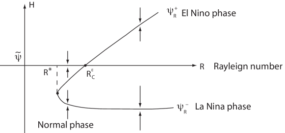
Figure 4.1. The transition diagram for the equatorial motion equations (2.3), $R^{*}$ is the saddle-node bifurcation point, $R^{\varepsilon}_{c}$ is the first critical Rayleigh number.

Theorem 4.2.

Let $\beta^{\varepsilon}_{1}(R)$ be complex near $R=R^{\varepsilon}_{c}$. Then the system (4.2) bifurcates from $(\psi,R)=(0,R^{\varepsilon}_{c})$ to a periodic solution $\psi_{R}(t)$ on $R^{\varepsilon}_{c}<R$, which is an attractor, and $\psi_{R}(t)$ can be expressed as

(4.6) $$\psi_{R}(t)=A_{R}(\cos\rho t\psi_{1}+\sin\rho t\tilde{\psi}_{1})+o(|A_{R}|,\varepsilon),$$

where $A_{R}=\alpha(R-R^{\varepsilon}_{c}),\alpha$ and $\rho$ are constants depending on $\varphi(x_{1})$, and $\psi_{1},\tilde{\psi}_{1}$ are first eigenfunctions of linearized equations of (2.3).

5. Concluding Remarks

In this article, a careful examination of the dynamic transitions and stability of the large-scale atmospheric flows over the tropics, associated with the Walker circulation and the ENSO, is given. The analysis and the results obtained show the following from the physical point of view.

First, Theorems 3.1, 4.1 and 4.2 provide the possible dynamical behaviors for the atmospheric circulation over the tropics. Theorem 3.1 is for the ideal case where the surface temperature profile is given as a constant, leading to a translation oscillation. Apparently, this result does not represent a realistic explanation to the ENSO.

Second, the time-periodic oscillation obtained in Theorem 4.2 does not represent the typical oscillation in the ENSO phenomena either, as the Walker circulation does not obey the zonal translational oscillation given by the periodic solutions.

Third, Theorem 4.1 does give a characterization of the ENSO, leading a correct oscillation mechanism of the ENSO between two metastable El Niño and La Niña events, which is further studied in [8].

Appendix A Dynamic Transition Theory for Nonlinear Systems

In this appendix we recall some basic elements of the dynamic transition theory developed by the authors [4, 7], which are used to carry out the dynamic transition analysis for the binary systems in this article.

A.1. New classification scheme

Let $X$ and $X_{1}$ be two Banach spaces, and $X_{1}\subset X$ a compact and dense inclusion. In this chapter, we always consider the following nonlinear evolution equations

(A.1) $$\left.\begin{aligned} &\frac{du}{dt}=L_{\lambda}u+G(u,\lambda),\\ &u(0)=\varphi,\end{aligned}\right.$$

where $u:[0,\infty)\rightarrow X$ is unknown function, and $\lambda\in\mathbb{R}^{1}$ is the system parameter.

Assume that $L_{\lambda}:X_{1}\rightarrow X$ is a parameterized linear completely continuous field depending continuously on $\lambda\in\mathbb{R}^{1}$, which satisfies

(A.2) $$\left.\begin{aligned} &L_{\lambda}=-A+B_{\lambda}&&\text{a sectorial operator},\\ &A:X_{1}\rightarrow X&&\text{a linear homeomorphism},\\ &B_{\lambda}:X_{1}\rightarrow X&&\text{a linear compact operator}.\end{aligned}\right.$$

In this case, we can define the fractional order spaces $X_{\sigma}$ for $\sigma\in\mathbb{R}^{1}$. Then we also assume that $G(\cdot,\lambda):X_{\alpha}\rightarrow X$ is $C^{r}(r\geq 1)$ bounded mapping for some $0\leq\alpha<1$, depending continuously on $\lambda\in\mathbb{R}^{1}$, and

(A.3) $$G(u,\lambda)=o(\|u\|_{X_{\alpha}}),\ \ \ \ \forall\lambda\in\mathbb{R}^{1}.$$

Hereafter we always assume the conditions (A.2) and (A.3), which represent that the system (A.1) has a dissipative structure.

Let the eigenvalues (counting multiplicity) of $L_{\lambda}$ be given by

$$\{\beta_{j}(\lambda)\in\mathbb{C}\ \ |\ \ j=1,2,\cdots\}$$

Assume that

(A.4) $$\text{Re}\ \beta_{i}(\lambda)\left\{\begin{aligned} &<0&&\text{ if }\lambda<\lambda_{0},\\ &=0&&\text{ if }\lambda=\lambda_{0},\\ &>0&&\text{ if }\lambda>\lambda_{0},\end{aligned}\right. \forall 1\leq i\leq m,$$

(A.5) $$\text{Re}\ \beta_{j}(\lambda_{0})<0 \forall j\geq m+1.$$

The following theorem is a basic principle of transitions from equilibrium states, which provides sufficient conditions and a basic classification for transitions of nonlinear dissipative systems. This theorem is a direct consequence of the center manifold theorems and the stable manifold theorems; we omit the proof.

Theorem A.1.

Let the conditions (A.4) and (A.5) hold true. Then, the system (A.1) must have a transition from $(u,\lambda)=(0,\lambda_{0})$, and there is a neighborhood $U\subset X$ of $u=0$ such that the transition is one of the following three types:

• Continuous Transition: there exists an open and dense set $\widetilde{U}_{\lambda}\subset U$ such that for any $\varphi\in\widetilde{U}_{\lambda}$, the solution $u_{\lambda}(t,\varphi)$ of (A.1) satisfies

  $$\lim\limits_{\lambda\rightarrow\lambda_{0}}\limsup_{t\rightarrow\infty}\|u_{\lambda}(t,\varphi)\|_{X}=0.$$

  In particular, the attractor bifurcation of (A.1) at $(0,\lambda_{0})$ is a continuous transition.

• Jump Transition: for any $\lambda_{0}<\lambda<\lambda_{0}+\varepsilon$ with some $\varepsilon>0$, there is an open and dense set $U_{\lambda}\subset U$ such that for any $\varphi\in U_{\lambda}$,

  $$\limsup_{t\rightarrow\infty}\|u_{\lambda}(t,\varphi)\|_{X}\geq\delta>0,$$

  where $\delta>0$ is independent of $\lambda$. This type of transition is also called the discontinuous transition.

• Mixed Transition: for any $\lambda_{0}<\lambda<\lambda_{0}+\varepsilon$ with some $\varepsilon>0$, $U$ can be decomposed into two open sets $U^{\lambda}_{1}$ and $U^{\lambda}_{2}$ ($U^{\lambda}_{i}$ not necessarily connected):

  $$\bar{U}=\bar{U}^{\lambda}_{1}+\bar{U}^{\lambda}_{2},\ \ \ \ U^{\lambda}_{1}\cap U^{\lambda}_{2}=\emptyset,$$

  such that

  $$\lim\limits_{\lambda\rightarrow\lambda_{0}}\limsup_{t\rightarrow\infty}\|u(t,\varphi)\|_{X}=0 \forall\varphi\in U^{\lambda}_{1},$$

  $$\limsup_{t\rightarrow\infty}\|u(t,\varphi)\|_{X}\geq\delta>0 \forall\varphi\in U^{\lambda}_{2}.$$

With this theorem in our disposal, we are in position to give a new dynamic classification scheme for dynamic phase transitions.

Definition A.1 (Dynamic Classification of Phase Transition).

The phase transitions for (A.1) at $\lambda=\lambda_{0}$ is classified using their dynamic properties: continuous, jump, and mixed as given in Theorem A.1, which are called Type-I, Type-II and Type-III respectively.

An important aspect of the transition theory is to determine which of the three types of transitions given by Theorem A.1 occurs in a specific problem. Hereafter we present a few theorems in this theory to be used in this article, and we refer interested readers to [10] for a complete description of the theory.

A.2. Transitions from simple eigenvalues

We consider the transition of (A.1) from a simple critical eigenvalue. Let the eigenvalues $\beta_{j}(\lambda)$ of $L_{\lambda}$ satisfy (A.4) and (A.5) with $m=1$. Then the first eigenvalue $\beta_{1}(\lambda)$ must be a real eigenvalue. Let $e_{1}(\lambda)$ and $e^{*}_{1}(\lambda)$ be the eigenvectors of $L_{\lambda}$ and $L^{*}_{\lambda}$ respectively corresponding to $\beta_{1}(\lambda)$ with

$$L_{\lambda_{0}}e_{1}=0,\ \ \ \ L^{*}_{\lambda_{0}}e^{*}_{1}=0,\ \ \ \ <e_{1},e^{*}_{1}>=1.$$

Let $\Phi(x,\lambda)$ be the center manifold function of (A.1) near $\lambda=\lambda_{0}$. We assume that

(A.6) $$<G(xe_{1}+\Phi(x,\lambda_{0}),\lambda_{0}),e^{*}_{1}>=\alpha x^{k}+o(|x|^{k}),$$

where $k\geq 2$ an integer and $\alpha\neq 0$ a real number.

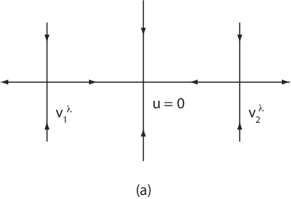
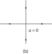
Figure A.1. Topological structure of the jump transition of (A.1) when $k$=odd and $\alpha>0$: (a) $\lambda<\lambda_{0}$; (b) $\lambda\geq\lambda_{0}$. Here the horizontal line represents the center manifold.

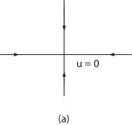
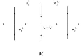
Figure A.2. Topological structure of the continuous transition of (A.1) when $k$=odd and $\alpha<0$: (a) $\lambda\leq\lambda_{0}$; (b) $\lambda>\lambda_{0}$.

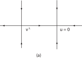
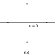
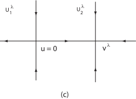
Figure A.3. Topological structure of the mixing transition of (A.1) when $k$=even and $\alpha\neq 0$: (a) $\lambda<\lambda_{0}$; (b) $\lambda=\lambda_{0}$; (c) $\lambda>\lambda_{0}$. Here $U^{\lambda}_{1}$ is the unstable domain, and $U^{\lambda}_{2}$ the stable domain.

Theorem A.2.

Assume (A.4) and (A.5) with $m=1$, and (A.6). If $k$=odd and $\alpha\neq 0$ in (A.6) then the following assertions hold true:

• If $\alpha>0$, then (A.1) has a jump transition from $(0,\lambda_{0})$, and bifurcates on $\lambda<\lambda_{0}$ to exactly two saddle points $v^{\lambda}_{1}$ and $v^{\lambda}_{2}$ with the Morse index one, as shown in Figure A.1.

• If $\alpha<0$, then (A.1) has a continuous transition from $(0,\lambda_{0})$, which is an attractor bifurcation as shown in Figure A.2.

• The bifurcated singular points $v^{\lambda}_{1}$ and $v^{\lambda}_{2}$ in the above cases can be expressed in the following form

  $$v^{\lambda}_{1,2}=\pm|\beta_{1}(\lambda)/\alpha|^{{1}/{k-1}}e_{1}(\lambda)+o(|\beta_{1}|^{{1}/{k-1}}).$$

Theorem A.3.

Assume (A.4) and (A.5) with $m=1$, and (A.6). If $k$=even and $\alpha\neq 0$, then we have the following assertions:

1. (A.1) has a mixed transition from $(0,\lambda_{0})$. More precisely, there exists a neighborhood $U\subset X$ of $u=0$ such that $U$ is separated into two disjoint open sets $U^{\lambda}_{1}$ and $U^{\lambda}_{2}$ by the stable manifold $\Gamma_{\lambda}$ of $u=0$ satisfying the following properties:

   1. $U=U^{\lambda}_{1}+U^{\lambda}_{2}+\Gamma_{\lambda}$,

   2. the transition in $U^{\lambda}_{1}$ is jump, and

   3. the transition in $U^{\lambda}_{2}$ is continuous. The local transition structure is as shown in Figure A.3.

2. (A.1) bifurcates in $U^{\lambda}_{2}$ to a unique singular point $v^{\lambda}$ on $\lambda>\lambda_{0}$, which is an attractor such that for any $\varphi\in U^{\lambda}_{2}$,

   $$\lim\limits_{t\rightarrow\infty}\|u(t,\varphi)-v^{\lambda}\|_{X}=0,$$

   where $u(t,\varphi)$ is the solution of (A.1).

3. (A.1) bifurcates on $\lambda<\lambda_{0}$ to a unique saddle point $v^{\lambda}$ with the Morse index one.

4. The bifurcated singular point $v^{\lambda}$ can be expressed as

   $$v^{\lambda}=-(\beta_{1}(\lambda)/\alpha)^{{1}/{(k-1)}}e_{1}+o(|\beta_{1}|^{{1}/{(k-1)}}).$$

A.3. Singular Separation

In this section, we study an important problem associated with the discontinuous transition of (A.1), which we call the singular separation.

Definition A.2.

1. An invariant set $\Sigma$ of (A.1) is called a singular element if $\Sigma$ is either a singular point or a periodic orbit.

2. Let $\Sigma_{1}\subset X$ be a singular element of (A.1) and $U\subset X$ a neighborhood of $\Sigma_{1}$. We say that (A.1) has a singular separation of $\Sigma$ at $\lambda=\lambda_{1}$ if

   1. (A.1) has no singular elements in $U$ as $\lambda<\lambda_{1}$ (or $\lambda>\lambda_{1}$), and generates a singular element $\Sigma_{1}\subset U$ at $\lambda=\lambda_{1}$, and

   2. there are branches of singular elements $\Sigma_{\lambda}$, which are separated from $\Sigma_{1}$ for $\lambda>\lambda_{1}$ (or $\lambda<\lambda_{1}$), i.e.,

      $$\lim\limits_{\lambda\rightarrow\lambda_{1}}\max_{x\in\Sigma_{\lambda}}\text{dist}(x,\Sigma_{1})=0.$$

A special case of singular separation is the saddle-node bifurcation defined as follows.

Definition A.3.

Let $u_{1}\in X$ be a singular point of (A.1) at $\lambda=\lambda_{1}$ with $u_{1}\neq 0$. We say that (A.1) has a saddle-node bifurcation at $(u_{1},\lambda_{1})$ if

1. the index of $L_{\lambda}+G$ at $(u_{1},\lambda_{1})$ is zero, i.e., ind$(-(L_{\lambda_{1}}+G),u_{1})=0$,

2. there are two branches $\Gamma_{1}(\lambda)$ and $\Gamma_{2}(\lambda)$ of singular points of (A.1), which are separated from $u_{1}$ for $\lambda>\lambda_{1}$ (or $\lambda<\lambda_{1})$, i.e., for any $u_{\lambda}\in\Gamma_{i}(\lambda)$ $(i=1,2)$ we have

   $$u_{\lambda}\rightarrow u_{1}\ \text{in}\ X\ \ \ \ \text{as}\ \lambda\rightarrow\lambda_{1},$$

   and

3. the indices of $u^{i}_{\lambda}\in\Gamma_{i}(\lambda)$ are as follows

   $$\text{ind}(-(L_{\lambda}+G),u_{\lambda})=\left\{\begin{aligned} &1&&\text{ if }u_{\lambda}\in\Gamma_{2}(\lambda),\\ &-1&&\text{ if }u_{\lambda}\in\Gamma_{1}(\lambda).\end{aligned}\right.$$

Intuitively, the saddle-node bifurcation is schematically shown as in Figure A.4, where the singular points in $\Gamma_{1}(\lambda)$ are saddle points and in $\Gamma_{2}(\lambda)$ are nodes, and the singular separation of periodic orbits is as in shown Figure A.5.

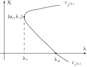
Figure A.4. Saddle-node bifurcation.

Figure A.5. Singular separation of periodic orbits.

For the singular separation we can give a general principle as follows, which provides a basis for singular separation theory.

Theorem A.4.

Let the conditions (A.4) and (A.5) hold true. Then we have the following assertions.

1. If (A.1) bifurcates from $(u,\lambda)=(0,\lambda_{0})$ to a branch $\Sigma_{\lambda}$ of singular elements on $\lambda<\lambda_{0}$ which is bounded in $X\times(-\infty,\lambda_{0})$ then (A.1) has a singular separation of singular elements at some $(\Sigma_{0},\lambda_{1})\subset X\times(-\infty,\lambda_{0})$.

2. If the bifurcated branch $\Sigma_{\lambda}$ consists of singular points which has index $-1$, i.e.,

   $$\text{ind}(-(L_{\lambda}+G),u_{\lambda})=-1\ \ \ \ \forall u_{\lambda}\in E_{\lambda},\ \ \ \ \lambda<\lambda_{0},$$

   then the singular separation is a saddle-node bifurcation from some $(u_{1},\lambda_{1})\in X\times(-\infty,\lambda_{0}).$

We consider the equation (A.1) defined on the Hilbert spaces $X=H,X_{1}=H_{1}$. Let $L_{\lambda}=-A+\lambda B$. For $L_{\lambda}$ and $G(\cdot,\lambda):H_{1}\rightarrow H$, we assume that $A:H_{1}\rightarrow H$ is symmetric, and

(A.7) $$<Au,u>_{H}\geq c\|u\|^{2}_{H_{{1}/{2}}},$$

(A.8) $$<Bu,u>_{H}\geq c\|u\|^{2}_{H},$$

(A.9) $$<Gu,u>_{H}\leq-c_{1}\|u\|^{p}_{H}+c_{2}\|u\|^{2}_{H},$$

where $p>2,c,c_{1},c_{2}>0$ are constants.

Theorem A.5.

Assume the conditions (A.3), (A.4) and (A.7)-(A.9), then (A.1) has a transition at $(u,\lambda)=(0,\lambda_{0})$, and the following assertions hold true:

1. If $u=0$ is an even-order nondegenerate singular point of $L_{\lambda}+G$ at $\lambda=\lambda_{0}$, then (A.1) has a singular separation of singular points at some $(u_{1},\lambda_{1})\in H\times(-\infty,\lambda_{0})$.

2. If $m=1$ and $G$ satisfies (A.6) with $\alpha>0$ if $k$=odd and $\alpha\neq 0$ if $k$=even, then (A.1) has a saddle-node bifurcation at some singular point $(u_{1},\lambda_{1})$ with $\lambda_{1}<\lambda_{0}$.

A.4. Transition and Singular Separation of Perturbed Systems

We consider the following perturbed equation of (A.1):

(A.10) $$\frac{du}{dt}=(L_{\lambda}+S^{\varepsilon}_{\lambda})u+G(u,\lambda)+T^{\varepsilon}(u,\lambda),$$

where $L_{\lambda}$ and $G_{\lambda}$ are as in (A.1), $S^{\varepsilon}_{\lambda}:X_{\sigma}\rightarrow X$ is a linear perturbed operator, $T^{\varepsilon}_{\lambda}:X_{\sigma}\rightarrow X$ a $C^{1}$ nonlinear perturbed operator, and $X_{\sigma}$ the fractional order space, $0\leq\sigma<1$. Also assume that $G_{\lambda},T^{\varepsilon}_{\lambda}$ are $C^{3}$ on $u$, and

(A.11) $$\left.\begin{aligned} &\|S^{\varepsilon}_{\lambda}\|<\varepsilon,\\ &\|T^{\varepsilon}_{\lambda}\|<\varepsilon,\\ &T^{\varepsilon}(u,\lambda)=o(\|u\|_{X_{\alpha}}).\end{aligned}\right.$$

Let (A.4) and (A.5) with $m=1$ hold true, $G(u,\lambda)=G_{2}(u,\lambda)+o(\|u\|^{2}_{X_{1}})$, where $G_{2}(\cdot,\lambda)$ is a bilinear operator, and

(A.12) $$b=<G_{2}(e,\lambda_{0}),e^{*}>\neq 0,$$

where $e\in X$ and $e^{*}\in X^{*}$ are the eigenvectors of $L_{\lambda}$ and $L^{*}_{\lambda}$ corresponding to $\beta_{1}(\lambda)$ at $\lambda=\lambda_{0}$ respectively.

We now consider the transition associated with the saddle-node bifurcation of the perturbed system (A.10). Let $h(x,\lambda)$ be the center manifold function of (A.1) near $\lambda=\lambda_{0}$. Assume that

(A.13) $$<G(xe+h(x,\lambda_{0}),\lambda_{0}),e^{*}>=b_{1}x^{3}+o(|x|^{3}),$$

where $b_{1}\neq 0$, and $e$ and $e^{*}$ are as in (A.12).

Then we have the following theorems.

Theorem A.6.

Let the conditions (A.4) and (A.5) with $m=1$, and (A.13) hold true, and $b_{1}<0$. Then there is an $\varepsilon>0$ such that if $S^{\varepsilon}_{\lambda}$ and $T^{\varepsilon}_{\lambda}$ satisfy (A.11), then the transition of (A.10) is either continuous or mixed. If the transition is continuous, then Assertions (2) and (3) of Theorem A.2 are valid for (A.10). If the transition is mixed, then the following assertions hold true:

1. (A.10) has a saddle-node bifurcation at some point $(u_{1},\lambda_{1})\in X\times(-\infty,\lambda^{\varepsilon}_{0})$, and there are exactly two branches

   $$\Gamma^{\lambda}_{i}=\{(u^{\lambda}_{i},\lambda)|\ \lambda_{1}<\lambda<\lambda^{\varepsilon}_{0}+\delta\}\qquad i=1,2,$$

   separated from $(u_{1},\lambda_{1})$ as shown in Figure A.4, which satisfy that

   $$\|u^{\lambda}_{2}\|_{X}\neq 0 \forall(u^{\lambda}_{2},\lambda)\in\Gamma^{\lambda}_{2},\ \ \ \ \lambda_{1}<\lambda<\lambda^{\varepsilon}_{0}+\delta,$$

   $$\lim_{\lambda\rightarrow\lambda^{\varepsilon}_{0}}\|u^{\lambda}_{1}\|_{X}=0 \forall(u^{\lambda}_{1},\lambda)\in\Gamma^{\lambda}_{1}.$$

2. There is a neighborhood $U\subset X$ of $u=0$, such that for each $\lambda$ with $\lambda_{1}<\lambda<\lambda^{\varepsilon}_{0}+\delta$ and $\lambda\neq\lambda^{\varepsilon}_{0},U$ contains only two nontrivial singular points $u^{\lambda}_{1}$ and $u^{\lambda}_{2}$ of (A.10).

3. For each $\lambda_{1}<\lambda<\lambda^{\varepsilon}_{0}+\delta,U$ can be decomposed into two open sets $\bar{U}=\bar{U}^{\lambda}_{1}+\bar{U}^{\lambda}_{2}$ with $U^{\lambda}_{1}\cap U^{\lambda}_{2}=\emptyset$, such that

   1. if $\lambda_{1}<\lambda<\lambda^{\varepsilon}_{0}$,

      $$0\in U^{\lambda}_{1},\ \ \ \ u^{\lambda}_{2}\in U^{\lambda}_{2},\ \ \ \ u^{\lambda}_{1}\in\partial U^{\lambda}_{1}\cap\partial U^{\lambda}_{2},$$

      with $u=0$ and $u^{\lambda}_{2}$ being attractors which attract $U^{\lambda}_{1}$ and $U^{\lambda}_{2}$ respectively, and

   2. if $\lambda^{\varepsilon}_{0}<\lambda<\lambda^{\varepsilon}_{0}+\delta$,

      $$u^{\lambda}_{1}\in U^{\lambda}_{1},\ \ \ \ u^{\lambda}_{2}\in U^{\lambda}_{2},\ \ \ \ 0\in\partial U^{\lambda}_{1}\cap\partial U^{\lambda}_{2},$$

      with $u^{\lambda}_{1}$ and $u^{\lambda}_{2}$ being attractors which attract $U^{\lambda}_{1}$ and $U^{\lambda}_{2}$ respectively.

4. Near $(u,\lambda)=(0,\lambda^{\varepsilon}_{0}),u^{\lambda}_{1}$ and $u^{\lambda}_{2}$ can be expressed as

   (A.14) $$\left.\begin{aligned} &u^{\lambda}_{1}=\alpha_{1}(\lambda,\varepsilon)e+o(|\alpha_{1}|),\\ &u^{\lambda}_{2}=\alpha_{2}(\lambda,\varepsilon)e+o(|\alpha_{2}|),\\ &\lim_{\lambda\rightarrow\lambda^{\varepsilon}_{0}}\alpha_{1}(\lambda,\varepsilon)=0,\\ &\alpha_{2}(\lambda^{\varepsilon}_{0},\varepsilon)\neq 0,\end{aligned}\right.$$

   where $e$ is as in (A.13).

Theorem A.7.

Assume the conditions (A.4) and (A.5) with $m=1$, and (A.13) with $b_{1}>0$. Then, there is an $\varepsilon>0$ such that when $S^{\varepsilon}_{\lambda}$ and $T^{\varepsilon}_{\lambda}$ satisfy (A.11), the transition of (A.10) is either jump or mixed. If it is jump transition, then Assertions (1) and (3) of Theorem A.2 are valid for (A.10). If it is mixed, then the following assertions hold true:

1. (A.10) has a saddle-node bifurcation at some point $(u_{1},\lambda_{1})\in X\times(\lambda^{\varepsilon}_{0},+\infty)$, and there are exactly two branches

   $$\Gamma^{\lambda}_{i}=\{(u^{\lambda}_{i},\lambda)|\ \lambda^{\varepsilon}_{0}-\delta<\lambda<\lambda_{1}\}\qquad(i=1,2),$$

   separated from $(u_{1},\lambda_{1})$, which satisfy

   $$\|u^{\lambda}_{2}\|_{X}=0 \forall(u^{\lambda}_{2},\lambda)\in\Gamma^{*}_{2},\ \ \ \ \lambda^{\varepsilon}_{0}-\varepsilon<\lambda<\lambda_{1},$$

   $$\lim\limits_{\lambda\rightarrow\lambda^{\varepsilon}_{0}}\|u^{\lambda}_{1}\|_{X}=0 \forall(u^{\lambda}_{1},\lambda)\in\Gamma^{\lambda}_{1}.$$

2. There is a neighborhood $U\subset X$ of $u=0$, such that for each $\lambda$ with $\lambda^{\varepsilon}_{0}-\delta<\lambda<\lambda_{1},U$ contains only two nontrivial singular points $u^{\lambda}_{1}$ and $u^{\lambda}_{2}$ of (A.10).

3. For every $\lambda^{\varepsilon}_{0}-\delta<\lambda<\lambda_{1},U$ can be decomposed into three open sets $\bar{U}=\bar{U}_{0}+\bar{U}_{1}+\bar{U}_{2}$ with $U_{i}\cap U_{j}=\emptyset$ $(i\neq j)$ such that

   1. if $\lambda^{\varepsilon}_{0}-\delta<\lambda<\lambda^{\varepsilon}_{0}$, then

      $$u=0\in U^{\lambda}_{0},\ \ \ \ u^{\lambda}_{i}\in\partial U^{\lambda}_{i}\cap\partial U^{\lambda}_{0}(i=1,2),$$

      with $u=0$ being an attractor which attracts $U^{\lambda}_{0}$ and $U^{\lambda}_{i}(i=1,2)$ two saddle points with the Morse index one, and

   2. if $\lambda^{\varepsilon}_{0}<\lambda<\lambda_{1}$, then

      $$u^{\lambda}_{1}\in U^{\lambda}_{1},\ \ \ \ u^{\lambda}_{2}\in\partial U^{\lambda}_{2}\cap\partial U^{\lambda}_{1},\ \ \ \ 0\in\partial U^{\lambda}_{1}\cap\partial U^{\lambda}_{0},$$

      with $u^{\lambda}_{1}$ being an attractor which attracts $U^{\lambda}_{1}$ and $u^{\lambda}_{2}$ and $u=0$ being saddle points with the Morse index one.

4. Near $(0,\lambda^{0}_{\varepsilon}),u^{\lambda}_{1}$ and $u^{\lambda}_{2}$ can be expressed by (A.14).

References

- [1] G. W. Branstator, A striking example of the atmosphere’s leading traveling pattern, J. Atmos. Sci., 44 (1987), pp. 2310–2323.
- [2] Y. Kushnir, Retrograding wintertime low-frequency disturbances over the north pacific ocean, J. Atmos. Sci., 44 (1987), pp. 2727–2742.
- [3] T. Ma and S. Wang, Dynamic bifurcation and stability in the Rayleigh-Bénard convection, Commun. Math. Sci., 2 (2004), pp. 159–183.
- [4] , Bifurcation theory and applications, vol. 53 of World Scientific Series on Nonlinear Science. Series A: Monographs and Treatises, World Scientific Publishing Co. Pte. Ltd., Hackensack, NJ, 2005.
- [5] , Geometric theory of incompressible flows with applications to fluid dynamics, vol. 119 of Mathematical Surveys and Monographs, American Mathematical Society, Providence, RI, 2005.
- [6] , Rayleigh-Bénard convection: dynamics and structure in the physical space, Commun. Math. Sci., 5 (2007), pp. 553–574.
- [7] , Stability and Bifurcation of Nonlinear Evolutions Equations, Science Press, 2007.
- [8] , El nino southern oscillation as sporadic oscillations between metastable states, submitted; see also arXiv:0812.4846v1, (2008).
- [9] , Superfluidity of helium-3, Physica A: Statistical Mechanics and its Applications, 387:24 (2008), pp. 6013–6031.
- [10] , Phase Transition Dynamics in Nonlinear Sciences, in preparation, 2009.
- [11] M. L. Salby, Fundamentals of Atmospheric Physics, Academic Press, 1996.
- [12] J. von Neumann, Some remarks on the problem of forecasting climatic fluctuations, in Dynamics of climate, R. L. Pfeffer, ed., Pergamon Press, 1960, pp. 9–12.