Abstract

We study the dynamical response of a single semiflexible polymer chain based on the theory developed by Hallatschek et al. for the wormlike-chain model. The linear viscoelastic response under oscillatory forces acting at the two chain ends is derived analytically as a function of the oscillation frequency $\omega$. We shall show that the real part $J^{\prime}$ of the complex compliance $J=J^{\prime}+iJ^{\prime\prime}$ in the low frequency limit $\omega\to 0$ is consistent with the static result of Marko and Siggia whereas the imaginary part $J^{\prime\prime}$ exhibits the power-law dependence $\omega^{+1/2}$. On the other hand, these compliances decrease as $\omega^{-7/8}$ for the high frequency limit $\omega\to\infty$. These are different from those of the Rouse dynamics. A scaling argument is developed to understand these novel results.

1 INTRODUCTION

The recent experimental advances in the manipulation of single molecules, such as optical tweezers and atomic force microscopy together with single-molecule fluorescence [1, 2, 3, 4], have enabled us to carry out mechanical and relaxational measurement in the nano-scale with piconewton sensitivity [5] in both equilibrium and non-equilibrium conditions. For example, static force-extension measurements of stretching of a single polymer chain have been carried out [6, 1, 7, 8]. As a non-equilibrium dynamics, the viscoelastic properties or the elastic and dissipative properties have also been studied [9, 13, 10, 11, 12]. Such experiments have revealed more detailed properties of single molecules that are difficult to obtain in bulk experiments due to the average taken over molecules and time. Therefore, these investigations lead to better understanding of the hierarchical structure of soft matter and the relationship between the molecular morphology and the functionality of biological molecules [4, 14].

One of the characteristic features of soft matter such as polymers or membranes is that they often have several length scales. Even in a single polymer chain if the chain is semi-flexible, there are at least two length scales, i.e., the persistence length and the total chain length. In the several experiments of single polymer chains, the semiflexibility, i.e., the stiffness, is an important factor [6, 9, 7]. In fact, the wormlike-chain model, which is a model of a semiflexible polymer [15, 16, 6], explains many experimental results considerably better than the flexible polymer chain model [17] particularly in the situation such as the highly-stretching limit in the force-extension measurement and the high wave-number limit of the dynamic structure factor, and so on [2, 6, 9, 7, 18, 19]. We emphasize that the rigidity effect can be enhanced in the above limits even for flexible polymers with a weak stiffness and that discrepancy appears between experiments and the theory based on a purely flexible model [19]. Therefore, investigation of the nonlinear dynamics due to the stiffness is necessary not only for semiflexible polymers but also for flexible polymers.

Despite the above fact as well as their fundamental interest in the field of mesoscopic physics and their importance to the material and biological application, semiflexible polymer chains have not been studied intensively especially for the dynamics because of the strong nonlinearity contained in the wormlike-chain model. Most of the theoretical studies of single polymers have been made in the limiting cases of either very flexible polymers or rigid rods [20]. So far, computer simulations have been carried out for a stiff chain or a semiflexible chain [22, 23, 24, 21].

Static theories of a semiflexible polymer chain are summarized as follows. Marko and Siggia derived the static force-extension relation based on the wormlike-chain model [6]. Other statistical properties, such as the distribution function of the end-to-end distance, have also been investigated [25, 26, 27]. Improvement of the wormlike-chain models has been proposed to examine the static properties [7, 28].

On the other hand, as mentioned above, analytical approaches to non-equilibrium dynamics of a semiflexible single polymer chain are limited. Some of the previous works have employed an approximation of linearization for the inextensibility constraint [29]. This linearization neglects non-uniformity of the line tension along the chain and has been applied to stretched polymers [18, 30, 31, 32].

Recently, Hallatschek et al. [33, 34] have formulated the force-extension theory for the wormlike-chain dynamics without linearization of the inextensibility condition introducing the concept of tension propagation. They consider a weakly bend situation and use a kind of multi-scale perturbation methods. The theory has been applied to the relaxation of an elongated chain after removing an external force [35, 36].

Finally, it is also mentioned that, as a previous theoretical method, the scaling approach to a semiflexible polymer chain [37, 34, 36], which was successful for flexible chains [38, 39, 40].

In the present paper, we develop the linear viscoelastic theory of a strongly pre-stretched single semiflexible polymer chain. We consider the situation such that an oscillatory force in addition to a constant force is applied to the two end of a wormlike-chain. Based on the method by Hallatschek et al. we derive the analytic representation of the complex compliance and the complex modulus. It will be shown that the frequency dependence is quite different from that of the Rouse model [40]. The preliminary results have been published in Ref. [41]. We apply a scaling analysis to understand the physical insight of the results.

The outline of the paper is as follows: In Section 2, we present the dynamical model of the wormlike-chain and the tension-propagation equation is derived based on the method by Hallatschek et al. [33, 34]. In Section 3, the complex compliance and the complex modulus are obtained analytically. In Section 4, the compliance and the modulus in the Rouse dynamics are given for comparison. In Section 5, the scaling approach is applied to both the weak-bending wormlike-chain dynamics and the Rouse dynamics. Summary and discussion are given in Section 6.

2 WORMLIKE-CHAIN MODEL AND THE RESPONSE TO THE OSCILLATORY FORCE

2.1 Dynamics of the wormlike-chain model

The effective Hamiltonian for the wormlike-chain is given by [15]

$$H_{WLC}=\frac{\kappa}{2}\int^{L}_{0}ds\left|\frac{d^{2}{\bm{r}}}{ds^{2}}\right|^{2},$$ (1)

with the constraint

$$|{\bm{r}^{\prime}}(s,t)|^{2}=1,$$ (2)

where $t$ denotes the time, $s$ is the length along the chain from one end, $L$ is the total length and ${\bm{r}}(s,t)$ represents the conformation of the chain. The positive constant $\kappa$ is the bending rigidity. The prime indicates the derivative with respect to $s$. The constraint (2) can be incorporated into the Hamiltonian as

$$H_{WLC}=\frac{\kappa}{2}\int^{L}_{0}ds\left|\frac{d^{2}{\bm{r}}}{ds^{2}}\right|^{2}+\frac{1}{2}\int_{0}^{L}dsf(s,t)\left|\frac{d{\bm{r}}}{ds}\right|^{2}\ ,$$ (3)

where $f(s,t)$ is the Lagrange multiplier for the constraint (2) and is interpreted as the line-tension. By assuming the over-damped motion, the stochastic equation of motion of a chain is given by

$$\zeta\partial_{t}{\bm{r}}(s,t)=-\kappa{\bm{r}^{\prime\prime\prime\prime}}+(f(s,t){\bm{r}^{\prime}}(s,t))^{\prime}+{\bm{g}}(s,t)+{\bm{\xi}(s,t)},$$ (4)

where the friction coefficient $\zeta$ is a $3\times 3$ matrix with the components $\zeta_{ij}$ ($i,j=x,y,z$) and ${\bm{g}}(s,t)$ represents the external force. The random force ${\bm{\xi}(s,t)}$ obeys the Gaussian white statistics:

$$<\xi_{i}(s,t)>=0,$$ (5)

$$<\xi_{i}(s,t)\xi_{j}(s^{\prime},t^{\prime})>=2k_{B}T\zeta_{ij}\delta(s-s^{\prime})\delta(t-t^{\prime})$$ (6)

with $k_{B}$ the Boltzmann coefficient and $T$ the absolute temperature. The equation of motion (4) is the same as that employed by Liverpool [42].

A remark is now in order. A stiff filament with an internal friction has been studied where the friction is supposed to arise from the internal conformation rearrangement of the filament with a finite radius [43]. It is emphasized here that we have not introduced such an additional friction in eq 4. As described below, the constraint eq 2 produces a strong nonlinear coupling between the longitudinal (parallel to the external force) and the transverse components of the conformation, which causes an energy dissipation whose magnitude is comparable with the typical elastic energy.

2.2 Weak bending approximation and multiple scale analysis

Now we follow the theory developed by Hallatschek, Frey and Kroy [33, 34]. They consider the situation such that the chain is elongated by the force $f$ applied to the ends. The smallness parameter is introduced as $\epsilon\equiv k_{B}T/(\kappa f)^{1/2}$. The conformation vector ${\bm{r}}(s,t)$ is divided into two components. One is parallel to the elongation direction (along the x-axis) and the other is perpendicular to it, i.e., ${\bm{r}}(s,t)=(s-r_{\parallel},{\bm{r}}_{\perp})$. The basic approximation is the weak bending approximation such that ${\bm{r}}_{\perp}^{\prime}(s,t)^{2}=O(\epsilon)\ll 1$. In this situation we have $r^{\prime}_{\parallel}=(1/2)({\bm{r}}^{\prime}_{\perp})^{2}+O(\epsilon^{2})$. Hallatschek et al. [33, 34] have introduced a concept of stored excess length defined by

$$\rho(s,t)=\frac{1}{2}({\bm{r}}^{\prime}_{\perp})^{2}.$$ (7)

Since the parallel component of the end-to-end distance is given by $R_{\parallel}\equiv L-(r_{\parallel}(L)-r_{\parallel}(0))$, we obtain the relation

$$<\Delta R_{\parallel}>(t)=-\int^{L}_{0}<\Delta\rho>(s,t)ds+o(\epsilon),$$ (8)

where $\Delta R_{\parallel}$ and $\Delta\rho$ indicate the deviation from some reference state and $<..>$ means a statistical average.

The Langevin equation (4) is split into two equations for $r_{\parallel}(s,t)$ and ${\bm{r}}_{\perp}(s,t)$ with the scalar friction coefficients $\zeta_{\parallel}$ and $\zeta_{\perp}$ respectively. The equation of the transverse motion is given by

$$\zeta_{\perp}\partial_{t}{\bm{r}}_{\perp}=-\kappa{\bm{r}^{\prime\prime\prime\prime}}_{\perp}+(f(s,t){\bm{r}^{\prime}}_{\perp})^{\prime}+{\bm{g}}_{\perp}+{\bm{\xi}_{\perp}}\ ,$$ (9)

where the external force ${\bm{g}}$ and the random force ${\bm{\xi}}$ are divided into the longitudinal and transverse components as ${\bm{g}}(s,t)=(g_{\parallel},{\bm{g}}_{\perp})$ and ${\bm{\xi}}(s,t)=(\xi_{\parallel},{\bm{\xi}}_{\perp})$, respectively. Taking the first derivative with respect to $s$ for the both sides of eq 4, the equation of the longitudinal motion is given by

$$\zeta_{\parallel} \partial_{t}r_{\parallel}^{\prime}=+(\zeta_{\parallel}-\zeta_{\perp})({\bm{r}^{\prime}}_{\perp}\cdot\partial_{t}{\bm{r}}_{\perp})^{\prime}$$

$$-\kappa r_{\parallel}^{\prime\prime\prime\prime\prime}-f^{\prime\prime}(s,t)+(f(s,t)r^{\prime}_{\parallel})^{\prime\prime}-g_{\parallel}^{\prime}-\xi_{\parallel}^{\prime}\ .$$ (10)

Note that the sign in front of $\xi_{\parallel}^{\prime}$ is minus because of the relation ${\bm{r}}=(s-r_{\parallel},{\bm{r}}_{\perp})$. In these expressions, $o(\epsilon^{1/2})$ terms and $o(\epsilon^{1})$ terms are neglected in eq 9 and eq 2.2, respectively. This set of equations is solved by a perturbation expansion together with the multiple scale analysis by introducing two scaled variables $s_{\text{s}}=s$ and $s_{\ell}=\epsilon^{1/2}s$. Noting that the ratio of the relaxation rate of $r_{\parallel}$ to that of ${\bm{r}}_{\perp}$ is $O(\epsilon^{-1/2})$, one may apply an adiabatic approximation for $r_{\parallel}$. Furthermore, the local equilibrium approximation is employed such that the degrees of freedom in the length scale $s_{\text{s}}$ is relaxed for a given constraint for the larger scale $s_{\ell}$. In this way, one obtains the following set of equations

$$-\frac{1}{k_{B}T}<\Delta\bar{\rho}(s,t)>=\int^{\infty}_{0}\frac{dq}{\pi}\left\{\frac{1-\exp(-A(q,s,t))}{\kappa q^{2}+f_{0}}\right.$$

$$\ \left.-\frac{2q^{2}}{\zeta_{\perp}}\int_{0}^{t}d\tilde{t}\exp\left(-A(q,s,t)+A(q,s,\tilde{t})\right)\right\}$$ (11)

and

$$<\Delta\bar{\rho}>(s,t)=-\frac{1}{\zeta_{\parallel}}\partial_{s}^{2}F(s,t)\ ,$$ (12)

where $q$ is the wave number representing modulations of the conformation ${\bm{r}}_{\perp}(s,t)$ and

$$F(s,t)=\int_{0}^{t}d\tilde{t}f(s,\tilde{t}),$$ (13)

$$A(q,s,t)=2q^{2}\Bigg{(}\kappa q^{2}t+F(s,t)\Bigg{)}/\zeta_{\perp}\ .$$ (14)

The quantity $<\Delta\bar{\rho}>(s,t)$ is the bulk value of $<\Delta\rho>(s,t)$. See Ref. [33] for details. We consider the situation such that the polymer chain is in a steady condition under a constant force $f_{0}$ applied at the ends till $t=0$ and then another time dependent force $\Delta f(s,t)$ is switched on at $t=0$, i.e., $f(s,t)=f_{0}+\Delta f(s,t)$ for $t>0$.

The tangential vector at the chain ends is approximated to be parallel to the direction of the external force. This is justified in the weak bend limit [33]. The time-integral of the force along the polymer chain is given by

$$F(s,t)=F_{0}(t)+\Delta F(s,t),$$ (15)

where $F_{0}(t)\equiv f_{0}t$ and

$$\Delta F(s,t)\equiv\int^{t}_{0}d\tilde{t}\Delta f(s,\tilde{t}).$$ (16)

2.3 Characteristic length and time

By comparing three terms in (3), one notes that there are three characteristic lengths

$$\ell_{p}=\frac{\kappa}{k_{B}T}$$ (17)

$$\ell_{f}=\frac{k_{B}T}{f}$$ (18)

$$\xi=\left(\frac{\kappa}{f}\right)^{1/2}\ ,$$ (19)

where $\ell_{p}$ is the persistence length of the chain and $\xi$ has a meaning of the “screening” length. In a linear response as we study in the present paper, the constant force $f_{0}$ should be used for $f$. The total length of the chain $L$ is also a characteristic length. The smallness parameter of the weak bending limit $\epsilon$ can be rewritten as follows

$$\epsilon=\frac{\xi}{\ell_{p}}=\frac{\ell_{f}}{\xi}=\left(\frac{k_{B}T}{\ell_{p}f}\right)^{1/2}\ .$$ (20)

This indicates that the magnitude of the characteristic lengths has a definite order for $\epsilon\ll 1$ as

$$\ell_{f}\ll\xi\ll\ell_{p}\lesssim L\ .$$ (21)

Hereafter we ignore the shortest one $\ell_{f}$.

Comparing each term in the Langevin equation (4), we obtain the following characteristic times

$$\tau_{1}=\frac{\ell^{4}\zeta_{\perp}}{\kappa}$$ (22)

$$\tau_{2}=\frac{\ell^{2}\zeta_{\perp}}{f}$$ (23)

with $\ell$ a length scale. Substituting $\ell=\xi$ into eq 23, we obtain

$$\tau_{\xi}=\frac{\kappa\zeta_{\perp}}{f^{2}}\ .$$ (24)

Substituting $\ell=\ell_{p}$ into eq 22, we have

$$\tau_{p}=\frac{\ell_{p}^{3}\zeta_{\perp}}{k_{B}T}=\frac{\kappa^{3}\zeta_{\perp}}{(k_{B}T)^{4}}\ .$$ (25)

Note that this is the only characteristic time which does not contain neither $f$ nor $L$.

2.4 Tension dynamics

In this subsection, we focus on the propagation of the line tension $f(s,t)$ or $F(s,t)$. Here it is mentioned that this concept itself can also be applied to a flexible polymer chain [44]. Combining eqs 11 and 12, the tension propagation equation is obtained as the closed form with respect to $F$;

$$\frac{\pi}{\zeta_{\parallel}k_{B}T}\partial_{s}^{2}F(s,t)=\int^{\infty}_{0}dq\left\{\frac{1-\exp(-A(q,s,t))}{\kappa q^{2}+f_{0}}\right.$$

$$\ \left.-\frac{2q^{2}}{\zeta_{\perp}}\int_{0}^{t}d\tilde{t}\exp\left(-A(q,s,t)+A(q,s,\tilde{t})\right)\right\}\ .$$ (26)

This equation is rewritten in terms of the dimensionless quantities as

$$K\partial_{\hat{s}}^{2}\hat{F}(\hat{s},\hat{t})=\int^{\infty}_{0}d\hat{q}\left\{\frac{1-\exp(-\hat{A}(\hat{q},\hat{s},\hat{t}))}{\hat{q}^{2}+1}\right.$$

$$\ \left.-2\hat{q}^{2}\int_{0}^{\hat{t}}d\tilde{t}\exp\left(-\hat{A}(\hat{q},\hat{s},\hat{t})+\hat{A}(\hat{q},\hat{s},\tilde{t})\right)\right\}\ ,$$ (27)

where

$$\hat{q}=\xi q\ ,$$ (28)

$$\hat{s}=\epsilon^{1/2}s\xi^{-1}\ ,$$ (29)

$$\hat{t}=t/\tau_{\xi}\ .$$ (30)

$K=\pi/\hat{\zeta}$ is just a numerical factor with $\hat{\zeta}\equiv\zeta_{\parallel}/\zeta_{\perp}$. The total length $L$ is now rescaled as $\hat{L}=\epsilon^{1/2}L\xi^{-1}$. The scaled functions $\hat{A}$ and $\hat{F}$ are given by

$$\hat{A}(\hat{q},\hat{s},\hat{t})=2\hat{q}^{2}\Bigg{(}\hat{q}^{2}\hat{t}+\hat{F}(\hat{s},\hat{t})\Bigg{)}$$ (31)

and

$$\hat{F}(\hat{s},\hat{t})=\frac{\xi^{2}}{\kappa\tau_{\xi}}F(s,t)=\int_{0}^{\hat{t}}d\tilde{t}\frac{f(\xi\hat{s},\tau_{\xi}\tilde{t})}{f_{0}}\ .$$ (32)

We assume that $\Delta f(s,t)$ is sufficiently small and apply the linearization approximation to (27). That is, we substitute (15) into (27) and retain the terms up to the first order with respect to $\Delta F$ so that we obtain

$$K\partial_{\hat{s}}^{2}\Delta\hat{F}+\int^{\hat{t}}_{0}d\tilde{t}\Delta\hat{F}(\hat{s},\hat{t}-\tilde{t})M(\tilde{t})=0,$$ (33)

where the memory function $M(\hat{t})$ is given by

$$M(\hat{t}) \equiv 4\int^{\infty}_{0}dq\left\{q^{4}e^{-2q^{2}(q^{2}+1)\hat{t}}-\frac{q^{2}}{q^{2}+1}\delta(\hat{t})\right\}.$$ (34)

The asymptotic behavior is given by $M(\hat{t})\sim\hat{t}^{-\beta}$ with $\beta=5/4$ for $\hat{t}\to 0$ and $\beta=5/2$ for $\hat{t}\to\infty$.

Equation (33) is to be solved under the boundary conditions specified by $\Delta F(0,t)$ and $\Delta F(L,t)$. In what follows, we consider the symmetric case that $\Delta F(0,t)=\Delta F(L,t)\equiv\Delta F(t)$. Applying the Laplace transformation with respect to $t$ to eq 33, we obtain

$$K\partial_{\hat{s}}^{2}\Delta\tilde{F}(\hat{s},z)+N(z)\Delta\tilde{F}(\hat{s},z)=0\ ,$$ (35)

where $\tilde{F}(\hat{s},z)$ denotes the Laplace transform of $\hat{F}(\hat{s},t)$ and

$$N(z)\equiv 4\int_{0}^{\infty}dq\left\{\frac{q^{4}}{2q^{2}(q^{2}+1)+z}-\frac{1}{2}\frac{q^{2}}{q^{2}+1}\right\}$$ (36)

is the Laplace transform of $M(t)$. The asymptotic form of $N(z)$ is given as follows. For $\omega\to\infty$, from eq 36 we obtain the following equations after some manipulation

$$\rm{Re}N(\pm i\omega\tau_{\xi}) =-2S_{1}(\omega\tau_{\xi})^{1/4},$$

$$\rm{Im}N(\pm i\omega\tau_{\xi}) =\mp 4S_{2}(\omega\tau_{\xi})^{1/4}$$ (37)

with $S_{1}=\int^{\infty}_{0}dq(4q^{8}+1)^{-1}\approx 0.863$ and $S_{2}=\int^{\infty}_{0}dqq^{4}(4q^{8}+1)^{-1}\approx 0.179$. It is readily shown that the Taylor expansion of N(z) with respect to $z$ breaks down and therefore N(z) is not analytic at $z=0$. The correct expansion is obtained after some manipulation as follows

$$N(\pm i\omega\tau_{\xi})=-2S_{3}(\omega\tau_{\xi})^{3/2}\mp iS_{4}(\omega\tau_{\xi})^{1}\ ,$$ (38)

where $S_{3}=\pi/8$ and $S_{4}=\pi/4$.

We consider the case that the force $\Delta f(t)$ at the boundaries is oscillatory as $\Delta f(t)=f_{A}\sin(\omega t)$ with the amplitude $f_{A}$ and the frequency $\omega$. The scaled form of $\Delta F$ at the boundaries is given by

$$\Delta\hat{F}(\hat{t})=(\omega\tau_{\xi})^{-1}\frac{f_{A}}{f_{0}}\left[1-\cos\left(\omega\tau_{\xi}\right)\right]$$ (39)

and the Laplace transform is

$$\Delta\tilde{F}(z)=\frac{f_{A}}{f_{0}}\frac{(\omega\tau_{\xi})}{z[z^{2}+(\omega\tau_{\xi})^{2}]}.$$ (40)

The solution of eq 35 can be represented as

$$\Delta\tilde{F}(\hat{s},z)=\Delta\tilde{F}(z)\times\frac{\cos\left(B(z)(2\hat{s}-\hat{L})\right)}{\cos\left(B(z)\hat{L}\right)},$$ (41)

where $B(z)=(N(z)/4K)^{1/2}$. One needs to evaluate the inverse Laplace transform of eq 41

$$\Delta\hat{F}(\hat{s},t)=\frac{1}{2\pi i}\int_{c-i\infty}^{c+i\infty}\Delta\tilde{F}(z)\frac{\cos\left(B(z)(2\hat{s}-\hat{L})\right)}{\cos\left(B(z)\hat{L}\right)}e^{zt}dz.$$ (42)

This will be carried out in the next section.

3 ANALYTICAL RESULTS

Now, we study the response of the end-to-end distance to the oscillatory force. The average end-to-end distance $\Delta R(t)$ which is a deviation from that of the steady state under the constant force $f_{0}$ is given by

$$\Delta R(t) =-\int^{L}_{0}ds<\Delta\bar{\rho}>(s,t)$$ (43)

$$=\frac{1}{\zeta_{\parallel}}\{\partial_{s}F(s,t)|_{s=L}-\partial_{s}F(s,t)|_{s=0}\}\ .$$ (44)

Hereafter, for abbreviation, we represent the statistical average of the end-to-end distance as $\Delta R(t)$ without the brackets $<\cdot>$, the bar $\bar{\cdot}$ and the parallel mark $\cdot_{\parallel}$. Substituting the solution (42) into eq 44 together with eq 32, we obtain the time evolution of the average end-to-end distance under the given boundary condition.

Since we are concerned with the asymptotic behavior $t\rightarrow+\infty$, we consider only the poles on the imaginary axis $z=0,\pm i\omega\tau_{\xi}$ to carry out the inverse Laplace transform. The final result can be written as

$$\frac{\Delta R(t)}{L}=\frac{f_{A}}{f_{0}}\left[\hat{J}^{\prime}(\omega)\sin(\omega t)-\hat{J}^{\prime\prime}(\omega)\cos(\omega t)\right]\ .$$ (45)

The scaled complex compliance is given by

$$\hat{J}^{\prime}(\omega)=-\frac{2D}{\omega\tau}\rm{Im}\Bigg{(}\bar{B}(i\omega\tau_{\xi})\tan(\bar{B}(i\omega\tau_{\xi}))\Bigg{)},$$ (46)

$$\hat{J}^{\prime\prime}(\omega)=-\frac{2D}{\omega\tau}\rm{Re}\Bigg{(}\bar{B}(i\omega\tau_{\xi})\tan(\bar{B}(i\omega\tau_{\xi}))\Bigg{)},$$ (47)

where $\bar{B}(z)=\alpha N(z)^{1/2}/2$ with complementary dimensionless constants

$$\alpha\equiv\frac{\hat{\zeta}^{1/2}(k_{B}T)^{1/2}f_{0}^{1/4}L}{\pi^{1/2}{\kappa}^{3/4}}=\sqrt{\frac{\hat{\zeta}}{\pi\epsilon}}\frac{L}{\ell_{p}}$$ (48)

and

$$D\equiv\frac{1}{2\pi^{2}}\frac{k_{B}T}{\sqrt{f_{0}\kappa}}=\frac{1}{2\pi^{2}}\epsilon\ .$$ (49)

The scaled elastic modulus $\hat{G}^{\prime}$ and the scaled loss modulus $\hat{G}^{\prime\prime}$ are obtained from $\hat{J}^{\prime}$ and $\hat{J}^{\prime\prime}$ as follows

$$\hat{G}^{\prime}(\omega)=\frac{\hat{J}^{\prime}(\omega)}{\hat{J}^{\prime}(\omega)^{2}+\hat{J}^{\prime\prime}(\omega)^{2}}\ ,$$ (50)

$$\hat{G}^{\prime\prime}(\omega)=\frac{\hat{J}^{\prime\prime}(\omega)}{\hat{J}^{\prime}(\omega)^{2}+\hat{J}^{\prime\prime}(\omega)^{2}}\ .$$ (51)

In the following, we introduce another characteristic time. The linearized eq 33 reduces to the following simple diffusion equation by employing the Markov approximation;

$$K\partial_{\hat{s}}^{2}\Delta\hat{F}(\hat{s},\hat{t})-\frac{\pi}{4}\partial_{\hat{t}}\hat{F}=0\ .$$ (52)

This implies that we may define a new relaxation time by the following form as the time scale of the slowest mode, just as the Rouse time in the continuous Rouse dynamics;

$$\tau\equiv\frac{k_{B}T\zeta_{\parallel}L^{2}}{4\pi^{2}{\kappa}^{1/2}f_{0}^{3/2}}=\frac{\alpha^{2}}{4\pi}\tau_{\xi}\ .$$ (53)

By this relation, the three parameters $\tau$, $\tau_{\xi}$ and $\alpha$ are not independent of each other. In Figures 1 and 2, we choose $\alpha$ and $\tau$ as the independent parameters.

We examine the limiting behavior of $\hat{J}^{\prime}$ and $\hat{J}^{\prime\prime}$. For the high frequency limit, substituting eq 37 into eqs 46 and 47 and after some manipulation, we obtain

$$\hat{J}^{\prime}(\omega) \sim\frac{4S_{1}^{1/2}b(k_{B}T)^{1/2}f_{0}}{\pi^{1/2}\hat{\zeta}^{1/2}\kappa^{5/8}\zeta_{\perp}^{7/8}L}\omega^{-7/8}\propto\kappa^{-5/8}(k_{B}T)^{+1/2}\omega^{-7/8}\ ,$$

$$\hat{J}^{\prime\prime}(\omega) \sim\frac{4S_{1}^{1/2}a(k_{B}T)^{1/2}f_{0}}{\pi^{1/2}\hat{\zeta}^{1/2}\kappa^{5/8}\zeta_{\perp}^{7/8}L}\omega^{-7/8}\propto\kappa^{-5/8}(k_{B}T)^{+1/2}\omega^{-7/8}$$ (54)

and

$$\hat{J}^{\prime}(\omega)/\hat{J}^{\prime\prime}(\omega)=b/a\approx 0.199\ ,$$ (55)

where $a\sim 0.721$ and $b\sim 0.142$ are the positive solutions of $(a+bi)^{2}=1/2+iS_{2}/S_{1}$. It should be noted that the unscaled complex compliance $J=L\hat{J}/f_{0}$ depends on neither $L$ nor $f_{0}$.

For the low frequency limit, substituting eq 38 into eqs 46 and 47 and after some manipulation, we obtain

$$\hat{J}^{\prime}(\omega) \sim\frac{1}{4}\frac{k_{B}T}{\sqrt{\kappa f_{0}}},$$ (56)

$$\hat{J}^{\prime\prime}(\omega) \sim\frac{k_{B}T\zeta_{\perp}^{1/2}}{4f_{0}^{3/2}}\omega^{+1/2}\propto\kappa^{0}(k_{B}T)^{+1}\omega^{+1/2}\ .$$ (57)

Note that (56) is consistent with the result of Marko and Siggia for the static stress-strain relation [6], which is given by

$$\frac{R(f_{0})}{L}=1-\frac{1}{2}\frac{k_{B}T}{\sqrt{\kappa f_{0}}}\ .$$ (58)

From this, we have

$$\frac{R(f_{0}(1+\delta))}{L}-\frac{R(f_{0})}{L}=\frac{\delta}{4}\frac{k_{B}T}{\sqrt{\kappa f_{0}}}+O(\delta^{2}).$$ (59)

Equations (46) and (47) give us the complex compliance as a function of $\omega$. Figures 1(a) and 1(b) show the compliances $\hat{J}^{\prime}$ and $\hat{J}^{\prime\prime}$ for $\alpha=1$ and $\alpha=100$, respectively. As mentioned above, the compliances exhibit the fractional power law behavior for the high frequency and $\hat{J}^{\prime}$ is consistent with the static result of the wormlike-chain for $\omega\to 0$. The difference for the simple Maxwell-like elasticity is more evident for $\hat{G}^{\prime}$ and $\hat{G}^{\prime\prime}$ as plotted for $\alpha=1$ in Figure 2 (a) and for $\alpha=100$ in Figure 2(b). Note that both $\hat{G}^{\prime}$ and $\hat{G}^{\prime\prime}$ increase as $\omega^{7/8}$ for $\omega\tau_{\xi}\gg 1$.

In addition, an intermediate region exists only if $\tau\gg\tau_{\xi}$ or $\alpha\gg 1$. From the definition (48), this condition is realized in the situation that the total chain length $L$ is much larger than $\epsilon^{1/2}\ell_{p}=\xi^{1/2}\ell_{p}^{1/2}.$ When this condition is satisfied, there is a finite interval of the intermediate region; $1/\tau\ll\omega\ll 1/\tau_{\xi}$. For example, in both Figure 1(b) and Figure 2(b), the interval $1\ll\omega\tau\lesssim 10^{2}$ corresponds to this region. In this region, the asymptotic form of $N$ is given by eq 38. Moreover, since $\bar{B}(i\omega\tau_{\xi})=\alpha N(i\omega\tau_{\xi})^{1/2}/2\sim(i\omega\tau)^{1/2}$, the imaginary part of $\bar{B}$ is very large. Therefore, we can approximate $\tan(\bar{B})$ by $+i$ and, substituting eq 38 into eqs 46 and 47, the compliance becomes

$$\hat{J}^{\prime}(\omega)\sim\omega^{-1/2}\frac{f_{0}^{1/4}(k_{B}T)^{1/2}}{\sqrt{2}L\zeta_{\parallel}^{1/2}\kappa^{1/4}}\left(1-\frac{1}{2}(\omega\tau_{\xi})^{1/2}\right)$$

$$\hat{J}^{\prime\prime}(\omega)\sim\omega^{-1/2}\frac{f_{0}^{1/4}(k_{B}T)^{1/2}}{\sqrt{2}L\zeta_{\parallel}^{1/2}\kappa^{1/4}}\left(1+\frac{1}{2}(\omega\tau_{\xi})^{1/2}\right)\ .$$ (60)

Thus, the compliance has the $\omega^{-1/2}$ dependence in the intermediate region.

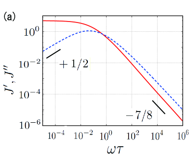
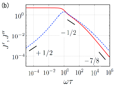
Figure 1: $\hat{J}^{\prime}$ and $\hat{J}^{\prime\prime}$ as a function of $\omega\tau$ for $D=1$ and (a) $\alpha=1.0$ and (b) $\alpha=100.0$. The full curve represents $\hat{J}^{\prime}$ whereas the broken curve represents $\hat{J}^{\prime\prime}$. The characteristic time $\tau$ is defined by eq 53.

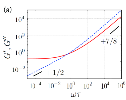
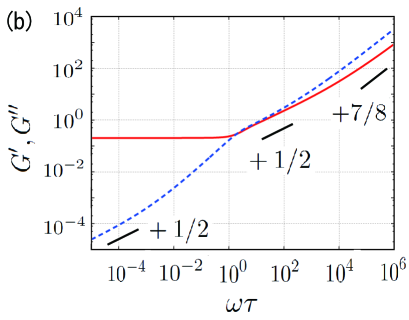
Figure 2: $\hat{G}^{\prime}$ and $\hat{G}^{\prime\prime}$ as a function of $\omega\tau$ for $D=1$ and (a) $\alpha=1.0$ and (b) $\alpha=100.0$. The full curve represents $\hat{G}^{\prime}$ whereas the broken curve represents $\hat{G}^{\prime\prime}$.

4 COMPARISON WITH ROUSE DYNAMICS

In this section, following the paper by Khatri and McLeish [40], we present the complex compliance for the Rouse model and compare it with the present result. The Rouse dynamics without internal friction is governed in the continuum limit by

$$\zeta\frac{d{\bm{r}}(n,t)}{dt}=k\frac{\partial^{2}{\bm{r}}(n,t)}{\partial n^{2}}+{\bm{f}}(n,t)+{\bm{\xi}}(n,t)\ ,$$ (61)

where $\zeta$ is the friction coefficient and the argument $n$ indicates the $n$-th monomer from one end, ${\bm{r}}(n)$ is the position vector of the $n$-th monomer and $k$ is the elastic coefficient of the linear spring between a pair of adjacent two monomers. It is noted that the argument $n$ and the number of monomer $N$ are treated as real numbers and satisfy $0\leqq n\leqq N$. Over-damped and Markov motion is assumed. Both end points are subjected to the external forces which have the same amplitude but the opposite direction

$${\bm{f}}(n,t)={\bm{f}}(t)\left[\delta(n-N)-\delta(n)\right]\ .$$ (62)

The last term ${\bm{\xi}}_{n}$ in eq 61 is the White Gaussian noise that satisfies the fluctuation dissipation relation of the second kind

$$<{\bm{\xi}}(n,t){\bm{\xi}}^{\dagger}(m,t^{\prime})>=2k_{B}T\zeta{\bm{I}}\delta(n-m)\delta(t-t^{\prime})\ ,$$ (63)

where ${\bm{I}}$ is the unit matrix and two adjacent matrices mean a tensor product.

We define the end-to-end distance as ${\bm{R}}(t)={\bm{r}}(N,t)-{\bm{r}}(0,t)$ and the deviation as $\Delta{\bm{R}}(t)={\bm{R}}(t)-{\bm{R}}(0)$. In the same way, the deviation of the external force is defined by $\Delta{\bm{f}}$. The complex compliance $J_{R}(\omega)=J_{R}^{\prime}(\omega)+iJ_{R}^{\prime\prime}(\omega)$ is defined through the relation

$$<\tilde{\Delta\bm{R}}>(i\omega)=J_{R}^{*}(\omega)\tilde{\Delta{\bm{f}}}(i\omega)\ ,$$ (64)

where the asterisk $\ast$ means the complex conjugate and $J_{R}^{*}(\omega)$ is given by [40]

$$J_{R}^{*}(\omega)=\frac{2N}{\pi k}\frac{\tanh\left(\frac{\pi}{2}\sqrt{i\omega\tau_{R}}\right)}{\sqrt{i\omega\tau_{R}}}\ ,$$ (65)

where $\tau_{R}$ is the Rouse relaxation time defined by

$$\tau_{R}=\frac{N^{2}\zeta}{\pi^{2}k}\ .$$ (66)

The function (65) is plotted in Figure 3 and the corresponding complex modulus $G_{R}$ is plotted in Figure 4.

From the expression (65), the asymptotic behavior is derived to compare with that of the weak-bending wormlike-chain dynamics. For $\omega\rightarrow\infty$, the complex compliance behaves as

$$J_{R}^{\prime}(\omega) \propto\omega^{-1/2}$$ (67)

$$J_{R}^{\prime\prime}(\omega) \propto\omega^{-1/2}\ ,$$ (68)

and for $\omega\rightarrow 0$

$$J_{R}^{\prime}(\omega) \rightarrow\text{const.}$$ (69)

$$J_{R}^{\prime\prime}(\omega) \propto\omega^{+1}\ .$$ (70)

These exponents are distinctly different from these obtained in the previous section, $-7/8$ in both $J_{R}^{\prime}$ and $J_{R}^{\prime\prime}$ as $\omega\rightarrow\infty$ and $+1/2$ in $J^{\prime\prime}$ as $\omega\rightarrow 0$. See eqs 54 and 57. Moreover, the viscoelastic behavior of the Rouse dynamics with internal friction is also examined by Khatri and McLeish [40], where the high frequency behavior is given by $J_{R}^{\prime}\propto\omega^{-2}$ and $J_{R}^{\prime\prime}\propto\omega^{-1}$. These are again different from the present results.

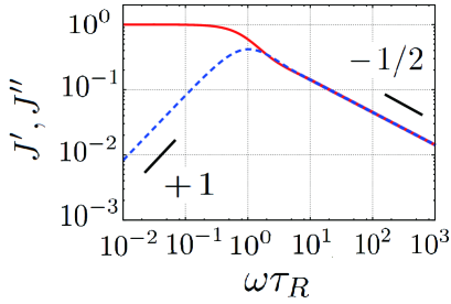
Figure 3: The complex compliance $J_{R}(\omega)=J_{R}^{\prime}(\omega)+iJ_{R}^{\prime\prime}(\omega)$ for the Rouse dynamics without internal friction. The full curve represents $J_{R}^{\prime}$ whereas the broken curve represents $J_{R}^{\prime\prime}$. The amplitude is scaled such that $J_{R}^{\prime}=1$ for $\omega\rightarrow 0$.

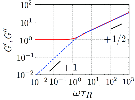
Figure 4: The complex modulus $G_{R}(\omega)=G_{R}^{\prime}(\omega)+iG_{R}^{\prime\prime}(\omega)$ for the Rouse dynamics without internal friction. The full curve represents $G_{R}^{\prime}$ whereas the broken curve represents $G_{R}^{\prime\prime}$. The amplitude is scaled such that $G_{R}^{\prime}=1$ for $\omega\rightarrow 0$.

5 SCALING APPROACH

5.1 Scaling form of $\Delta R(t)$

In this section, we apply the scaling analysis in order to explain the behavior of complex compliances for both high and low frequency limits.

All the parameters are scaled out in eqs 27 and 29. Therefore, the parameters appear only through eq 32 and through the boundary condition which contains $L$. The scaled form of $L$ is given by $\hat{L}=\epsilon^{1/2}L\xi^{-1}$. These facts together with eq 44 give us the following scaling property of $\Delta R$;

$$\Delta R(t)=\epsilon^{1/2}\xi^{-1}\tau_{\xi}f\zeta^{-1}Q(\epsilon^{1/2}L\xi^{-1},t/\tau_{\xi})\ ,$$ (71)

where $Q(x,y)$ is an unknown function whose asymptotic form is to be determined. This scaling form (71) is very crucial to investigate the asymptotic behavior of the compliance and the modulus as shown below.

5.2 Complex compliance for the high frequency limit

The exponent $7/8$ exhibited by $J^{\prime}$ and $J^{\prime\prime}$ for $\omega\rightarrow\infty$ obtained in eq 54 can be understood by the following scaling analysis. In the linear response regime, the dimensionless function $Q$ in eq 71 should be proportional to $f_{A}/f_{0}$. At the high frequency limit, the effect of the external force is expected to be localized near the two ends and hence the compliance $J$ should not depend on $L$. Therefore, from eq 71, the compliance takes the following form

$$f_{A}J(\omega)\sim\frac{f_{A}}{f}\epsilon^{1/2}\xi^{-1}\tau_{\xi}f\zeta^{-1}(\omega\tau_{\xi})^{-z}$$ (72)

with an unknown exponent $z$. Substituting the definitions of $\xi$, $\epsilon$ and $\tau_{\xi}$ given, respectively, by (19), (20) and (24) into eq 72 yields

$$f_{A}J(\omega)\sim f_{A}f^{-7/4+2z}\kappa^{1/4-z}(k_{B}T)^{1/2}\zeta^{-z}\omega^{-z}\ .$$ (73)

We can require that the compliance is independent of the screening length $\xi$ (and hence $f$) in the high frequency limit. This is because the relaxation of the chain has the factor $\kappa q^{4}+fq^{2}$ as can be seen from eq 4 or eqs 14 and 15 and hence $\kappa$ is relevant for the high frequency ($fq^{2}$ is irrelevant). This requirement gives us

$$z=\frac{7}{8}\ .$$ (74)

The scaling analysis in the Rouse dynamics is different from the above because of the absence of the local length scale, i.e., the persistence length $\ell_{p}$. The Rouse model has only one length scale, the root of the mean square end-to-end distance $\sigma$. When no external force is present, it is given by [20]

$$\sigma\sim\left(\frac{k_{B}T}{k}\right)^{1/2}N^{1/2}\ .$$ (75)

Therefore the dimensional analysis tells us that the deviation of the end-to-end distance should obey

$$\Delta R\sim\sigma\frac{\sigma f_{A}}{k_{B}T}\hat{J}(\omega\tau_{R})e^{i\omega t}$$ (76)

with the external force

$$f(t)=f_{A}e^{i\omega t}\ .$$ (77)

Assuming that $\hat{J}$ has a power law behavior $\hat{J}(\omega\tau_{R})\sim(\omega\tau_{R})^{-z}$ as $\omega\rightarrow\infty$. The complex compliance becomes

$$f_{A}J(\omega)\sim\sigma\frac{\sigma f_{A}}{k_{B}T}(\omega\tau_{R})^{-z}\sim f_{A}N^{1-2z}\omega^{-z}k^{z-1}\zeta^{-z}\ .$$ (78)

In the high frequency limit, the response is localized and the compliance should be independent of $N$ so that the exponent is determined uniquely as $z=1/2$ or

$$J(\omega)\propto\omega^{-1/2}\ .$$ (79)

This is the argument given by Khatri et al. [40].

5.3 Complex compliance for the low frequency limit

The exponent $1/2$ exhibited by $J^{\prime\prime}$ for $\omega\rightarrow 0$ obtained in eq 57 can be understood as follows. In the low frequency limit, the effect of the external force is extended almost uniformly to the whole chain. Therefore, we can require that $J$ is proportional to $L$ so that

$$f_{A}J(\omega)=\frac{f_{A}}{f}\epsilon^{1/2}\xi^{-1}\epsilon^{1/2}L\xi^{-1}\tau_{\xi}f\zeta^{-1}(\omega\tau_{\xi})^{z}\ .$$ (80)

The real part $J^{\prime}$ is independent of the frequency for $\omega\to 0$ and hence $z=0$ whereas the imaginary part $J^{\prime\prime}$ should be independent of $\kappa$ for $\omega\to 0$. As mentioned above, the relaxation of the chain has the factor $\kappa q^{4}+fq^{2}$ and hence $\kappa$ is irrelevant for the low frequency. Therefore, substituting the definitions of $\xi$, $\epsilon$ and $\tau_{\xi}$ given, respectively, by (19), (20) and (24) into eq 80, it is found that the exponent is given by

$$z=\frac{1}{2}$$ (81)

so that $J^{\prime\prime}\propto k_{B}T\omega^{1/2}$. Note that, from eq 73, $J^{\prime\prime}$ at the high frequency limit is proportional to $(k_{B}T)^{1/2}$ whereas it is proportional to $k_{B}T$ at the low frequency limit.

In contrast, the complex compliance in the Rouse dynamics is analytic in the $\omega\rightarrow 0$ limit. This fact is clear from the expression (65). This should be compared with that of the wormlike-chain dynamics (56) and (57) where the function N(z) in $\bar{B}(z)$ contains a non-analyticity as eq 38.

6 SUMMARY AND DISCUSSION

In summary, we have developed the analytical theory of the viscoelasticity of single semiflexible polymer chains and have obtained the linear compliance which has a frequency dependence characteristic to the semiflexible chain. In particular, it is found that the asymptotic behavior of the compliance obeys as $J^{\prime},J^{\prime\prime}\propto\omega^{-7/8}$ for $\omega\to\infty$ whereas $J^{\prime\prime}\propto\omega^{+1/2}$ for $\omega\tau\ll 1$. These are distinctly different from the results of the Rouse dynamics. The constant of $J_{R}^{\prime}$ for $\omega=0$ given by eq 56 is also different from that of the flexible chain.

The theory assumes weakness of the bending parameter $\epsilon\ll 1$ which guarantees the scale separation. This is due to the fact that the characteristic length parallel to the stretched chain $\ell_{\parallel}\sim\Delta s$ and the characteristic wave length $q^{-1}\sim\ell_{\perp}$ satisfy

$$\frac{\ell_{\perp}}{\ell_{\parallel}}\sim\frac{q^{-1}}{\Delta s}\sim\epsilon^{1/2}\frac{\hat{q}^{-1}}{\Delta\hat{s}}\ll 1\ ,$$ (82)

where the scaling forms (28) and (29) have been used. It is emphasized that, for $\omega\to\infty$, the scale separation is valid without assuming the smallness of $\epsilon$ because of the fact that $\ell_{\parallel}\propto\omega^{-1/8}\gg\ell_{\perp}\propto\omega^{-1/4}$. This fact is verified by eqs 35 and 36.

Now we discuss the relation between the present results and those obtained by Hallatschek et al. who have considered the relaxation of the end-to-end distance after step-wise change of the external force [34, 36]. They have predicted that both in the stretching case and in the release case the end-to-end distance behaves as

$$<\Delta R_{\parallel}(t)>\propto f\kappa^{-5/8}(k_{B}T)^{-1/2}t^{7/8}\ ,$$ (83)

where $t\ll t_{f}\sim\zeta\kappa f^{-2}$. The exponent $7/8$ is the same as that in the high-frequency limit in eq 54. At a short interval after the force change, its effect is localized near the chain ends which is small compared with both the persistence length (17) and the screening length (19). In fact, we can show that eq 83 is consistent with our eq 54 as follows. In the linear response theory the relaxation function $\psi(t)$ and response function $\phi(t)$ are related to each other as $\phi(t)=-d\psi(t)/dt$. The complex compliance is the Fourier-Laplace transform of the response function $\phi$ and hence $J(\omega)=\psi(0)+i\omega\int_{0}^{+\infty}dte^{i\omega t}\psi(t)$. Therefore, we have the following relation $J(\omega)\sim\psi(1/\omega)$ and $\hat{J}(\omega)=fJ/L\sim\langle\Delta R_{\parallel}(1/\omega)\rangle/L$.

In the intermediate time region $t_{L}\gg t\gg t_{f}$ with the crossover time $t_{L}$ defined through $\ell_{\parallel}(t_{L})=L$, Hallatschek et al. have obtained [34]

$$<\Delta R_{\parallel}(t)>\propto f^{3/4}\kappa^{-1/2}(k_{B}T)^{1/2}t^{3/4}$$ (84)

for a pulling situation and

$$<\Delta R_{\parallel}(t)>\propto f^{1/4}\kappa^{-1/4}(k_{B}T)^{1/2}t^{1/2}$$ (85)

for a release situation. We have no results corresponding to eq 84 since this contains a nonlinear effect of the applied force. On the other hand, the exponent 1/2 in eq 85 corresponds to eq 60 in the present paper. Actually one can verify that not only the exponent but also the coefficient in eq 85 is consistent with our result. This implies that the expression (85) is free from the nonlinearity between the force-strain relation.

Finally we mention a theoretical study which gives us the exponent 1/2 in the compliance. Caspi et al. have investigated the mean square displacement of a single monomer of a prestressed semiflexible network [47]. They have obtained

$$<\Delta h^{2}(x,t)>\propto\frac{k_{B}T}{\nu^{1/2}\eta^{1/2}}t^{1/2}\ ,$$ (86)

where $h(x,t)$ denotes the undulation amplitude, $\nu$ the line tension, $\eta$ the solvent viscosity and $L$ the total chain length. Equation (86) holds in the time region $4\pi\eta\kappa/\nu^{2}\ll t\ll\eta L^{2}/\nu$. Furthermore, they have shown that the effective time dependent friction $\zeta_{e}(t)$ satisfies the generalized Einstein relation

$$\frac{k_{B}T}{\zeta_{e}(t)}=\frac{<\Delta h^{2}(t)>}{2t}\ .$$ (87)

Combining eqs 86 and 87, one obtains the complex compliance ($J\propto t/\zeta_{e}(t)$)

$$J(\omega)\propto\nu^{-1/2}\eta^{-1/2}\omega^{-1/2}\ .$$ (88)

Some experiments of semiflexible networks support the exponent 1/2 [47, 48]. It is mentioned, however, that the physical of this result is different from our present result for semi-flexible chain given by eq 60. This fact is clear because the coefficient in eq 88 does not contain $k_{B}T$ whereas our expression eq 60 is proportional to $(k_{B}T)^{1/2}$.

Now we comment on the several effects which have not been considered in the present paper. The hydrodynamic effect has not been investigated quantitatively in a nonlinear wormlike-chain although it is expected to be not so strong in a strongly stretched semi-flexible chain. The previous studies of the hydrodynamic effect in the linearized wormlike-chain dynamics [18, 19, 31, 32] should be extended to apply to the present theory. The internal friction considered in the Rouse dynamics [40] should also be extended to the semi-flexible chains. In addition, the helical wormlike-chain model, which contains the torsional energy, has been studied in dilute solutions [26, 52, 53]. This torsional effect may affect the viscoelastic properties of single polymer chains.

Before closing this article, we make an estimation of the characteristic times $\tau_{\xi}$ and $\tau$ defined by eqs 24 and 53 respectively. The data for $\lambda$-DNA in an aqueous solution are as follows [45, 46, 34]

$$\ell_{P}\sim 50[\text{nm}],$$

$$L\sim 20[\text{$\mu$m}],$$

$$\zeta_{\perp}\sim 1.3\times 10^{-3}[\text{Pa s}]=1.3\times 10^{-3}[\text{pN$\cdot$s/$\mu$m${}^{2}$}]\ .$$

For these values together with $\hat{\zeta}\sim 1/2$ for a rigid rod [20] and the room temperature $k_{B}T\sim 4.1[\text{pN}\cdot\text{nm}]$, and for the external force $f_{0}\sim 10[\text{pN}]$ the characteristic times are given by

$$\tau_{\xi}\sim 2.7\times 10^{-9}[\text{s}]$$

$$\tau\sim 6.0\times 10^{-5}[\text{s}]=60[\text{$\mu$s}]$$

and the constant $\alpha\sim 5.3\times 10^{2}$. We expect that the frequency of the order of 60 [$\mu$s] is accessible by atomic force microscopy and that the present predictions can be detected experimentally.

References

• [1] Wang, M. D.; Yin, H.; Landick, R.; Gelles, J.; Block, S.M. BioPhys. J. 1997,72, 1335.
• [2] Ladoux, B.; Quivy, J.; Doyle, P. S.; Almouzni, G.; Viovy, J. Science Prog. 2001, 84, 267.
• [3] Cocco, S.; Marko, J. F.; Monasson, R. C. R. Physique 2002, 3, 569.
• [4] Ritort, F. J. Phys.:Condens. Matter 2006,18, R531.
• [5] Strick, T.; Allemand, J.; Croquette, V.; Bensimon, D. Physics Today 2001, 46.
• [6] Marko, J. F.; Siggia, E. D. Macromolecules 1995, 28, 8759.
• [7] Bouchiat, C.; Wang, M. D.; Allemand, J. -F.; Strick, T.; Block, S. M.; Croquette, V. Biophys. J. 1999, 76, 409.
• [8] Murayama, Y.; Wada, H.; Ishida, R.; Sano, M. Prog. Theor. Phys. Supp. 2006, 165, 144.
• [9] Sakai, Y.; Ikehara, T.; Nishi, T.; Nakajima, K.; Hara, M. Appl. Phys. Lett. 2002, 81, 724.
• [10] Kawakami, M.; Byrne, K.; Khatri, B.; McLeish, T. C. B.; Radford, S. E.; Smith, D. A. Langmuir 2004, 20, 9299.
• [11] Kawakami, M.; Byrne, K.; Khatri, B.; McLeish, T. C. B.; Radford, S. E.; Smith, D. A. Langmuir 2005, 21, 4765.
• [12] Kawakami, M.; Byrne, K.; Khatri, B.; Brockwell, D. J.; Radford, S. E.; Smith, D. A. Biophys. J. 2006, 91, L16.
• [13] Khatri, B. S.; Kawakami, M.; Byrne, K.; Smith, D. A.; McLeish, T. C. B. Biophys. J. 2007, 92, 1825.
• [14] Yamada, A.; Kubo, K.; Nakai, T.; Yoshikawa, K.; Tsumoto, K. Appl. Phys. Lett. 2005, 86, 223901.
• [15] Kratky, O.; Porod, G. Rec. Trav. Chim. Pays-Bas 1949, 68, 1106.
• [16] Fixman, M.; Kovac, J. J. Chem. Phys 1973, 58, 1564.
• [17] Edwards, S. F. Proc. Phys. Soc. 1966, 88, 265.
• [18] Winkler, R. G. Phys. Rev. Lett. 1999, 82, 1843.
• [19] Harnau, L.; Winkler, R. G.; Reineker, P. J. Chem. Phys. 1996, 104, 6355.
• [20] Doi, M.; Edwards, S. F. The Theory of Polymer Dynamics; Clarendon Press: Oxford, 1986.
• [21] Morrison, G.; Hyeon, C.; Toan, N. M.; Ha, B. -Y.; Thirumalai, D. Macromolecules 2007, 40, 7343.
• [22] Somasi, M.; Khomami, B.; Woo, N. J.; Hur, J. S.; Shaqfeh, E. S. G. J. Non-newtonian Fluid Mech. 2002, 108, 227.
• [23] Yoshinaga, N.; Yoshikawa, K.; Ohta, T. Eur. Phys. J. E 2005, 17, 485.
• [24] Chattopadhyay, A. K.; Marenduzzo, D. Phys. Rev. Lett. 2007, 98, 088101.
• [25] Wilhelm, J.; Frey, E. Phys. Rev. Lett. 1996, 77, 2581.
• [26] Chirikjian, G. S.; Wang, Y. Phys. Rev. E 2000, 62, 880.
• [27] Hamprecht, B.; Keinert, H. Phys. Rev. E 2005, 71, 031803.
• [28] Winkler, R. G. J. Chem. Phys 2003, 118, 2919.
• [29] Saito, N.; Takahashi, K.; Yunoki, Y. J. Phys. Soc. Jpn. 1967, 22, 1.
• [30] Bohbot-Raviv, Y.; Zhao, W. A.; Feingold, M.; Wiggins, C. H.; Granek, R. Phys. Rev. Lett. 2004, 92, 9.
• [31] Winkler, R. G.; Keller, S.; RΓΆder, J. O. Phys. Rev. E 2006, 73, 041919.
• [32] Winkler, R. G. J. Chem. Phys 2007, 127, 054904.
• [33] Hallatschek, O.; Frey, E.; Kroy, K. Phys. Rev. E 2007, 75, 031905.
• [34] Hallatschek, O.; Frey, E.; Kroy, K. Phys. Rev. E 2007, 75, 031906.
• [35] Obermayer, B.; Hallatschek, O. Phys. Rev. Lett. 2007, 99, 098302.
• [36] Obermayer, B.; Hallatschek, O. Frey, E.; Kroy, K. Eur. Phys. J. E 2007, 23, 375.
• [37] Everaers, R.; JΓΌlicher, F.; Ajdari, A.; Maggs, A. C. Phys. Rev. Lett. 1999, 82, 3717.
• [38] de Gennes, P. G. Scaling Concepts in Polymer Physics; Cornell University Press: New York, 1979.
• [39] Pincus, P. Macromolecules 1976, 9, 386.
• [40] Khatri, B. S.; McLeish, T. C. B. Macromolecules 2007, 40, 6770.
• [41] Hiraiwa, T.; Ohta, T. J. Phys. Soc. Jpn. 2008, 77, 023001.
• [42] Liverpool, T. B. Phys. Rev. E 2005, 72, 021805.
• [43] Poirier, M. G.; Marko, J. F. Phys. Rev. Lett. 2002, 88, 228103.
• [44] Sakaue, T. Phys. Rev. E 2007, 76, 021803.
• [45] Quake, S. R.; Babcock, H.; Chu, S. Nature 1997, 388, 151.
• [46] Maier, B.; Seifert, U.; RΓ€dler, J. O. Europhys. Lett. 2002, 60, 622.
• [47] Caspi, A.; Elbaum, M.; Granek, R.; Lachish, A.; Zbaida, D. Phys. Rev. Lett. 1998, 80, 1106.
• [48] Mizuno, D.; Tardin, C.; Schmidt, C. F.; MacKintosh, F. C. Science 2007, 15, 370.
• [49] Majumdar, A.; Suki, B.; Rosenblatt, N.; Alencar, A. M.; StamenoviΔ‡, D. Phys. Rev. E 2008, 78, 041922.
• [50] Morse, D. C. Macromolecules 1998, 31, 7044.
• [51] Gittes, F.; MacKintosh, F. C. Phys Rev E. 1998, 58, R1241.
• [52] Yamakawa, H.; Fujii, M. J. Chem. Phys. 1976, 64, 5222.
• [53] Yamakawa, H.; Yoshizaki, T. J. Chem. Phys. 1981, 75, 1016.