Polarization Evolution in A Strongly Magnetized Vacuum: QED Effect and Polarized X-ray Emission from Magnetized Neutron Stars

Abstract

X-ray photons emitted from the surface or atmosphere of a magnetized neutron star are highly polarized. However, the observed polarization may be modified due to photon propagation through the star’s magnetosphere. For photon frequencies much larger than the typical radio frequency, vacuum birefringence due to strong-field quantum electrodynamics dominates over the plasma effect. We study the evolution of photon polarization in the magnetized QED vacuum of a neutron star magnetosphere, paying particular attention to the propagation effect across the quasi-tangential (QT) point, where the photon momentum is nearly aligned with the magnetic field. In agreement with previous studies, we find that in most regions of the magnetosphere, the photon polarization modes are decoupled due to vacuum birefringence, and therefore a large net linear polarization can be expected when the radiation escapes the magnetosphere. However, we show that the X-ray polarization may change significantly when the photon passes through the QT region. When averaging over a finite emission area, the net effect of QT propagation is to reduce the degree of linear polarization; the reduction factor depends on the photon energy, magnetic field strength, geometry, rotation phase and the emission area, and can be more than a factor of two. We derive the general conditions under which the QT propagation effect is important, and provide an easy-to-use prescription to account for the QT effect for most practical calculations of X-ray polarization signals from magnetic neutron stars. For a neutron star with a dipole magnetic field, the QT effect can be important for emission from the polar cap for certain magnetic field and energy ranges, and is negligible for emission from the entire stellar surface.

1 Introduction

Thermal, surface emission from neutron stars (NSs) has the potential of providing invaluable information on the physical properties and evolution of NSs (equation of state at super-nuclear densities, cooling history, magnetic field, surface composition, different populations; see, e.g., Yakovlev & Pethick 2004; Harding & Lai 2006). With X-ray telescope such as Chandra and XMM-Newton, the last decade has seen significant observational progress, revealing the surface magnetic field geometry of isolated pulsars with phase-resolved spectroscopy, and constraining the cooling physics from thermal emission of young NSs in supernova remnants (e.g., Kaspi et al. 2006). In addition, thermal emission from seven isolated, radio-quiet NSs has been studied in detail, revealing absorption features in their spectra in many cases (see, e.g., van Kerkwijk & Kaplan 2007; Kaplan 2008).

It has been recognized that in addition to imaging, timing and spectroscopy, X-ray polarimetry provides a new way to study many high-energy astrophysical sources, particularly magnetic NSs. Recent advances in detector technology suggest that polarimetry study of X-ray sources holds great promise in the future (e.g., Costa et al. 2008; Swank et al. 2008).

The surface emission from magnetized NSs (with $B\mathrel{\raise 1.29167pt\hbox{$>$}\mkern-14.0mu\lower 2.58334pt\hbox{$\sim$}}10^{12}$ G) is highly polarized (e.g., Gnedin & Sunyaev 1974; Meszaros et al. 1988; Pavlov & Zavlin 2000) for the following reason. In the magnetized plasma that characterizes NS atmospheres, X-ray photons propagate in two normal modes: the ordinary mode (O-mode, or $\parallel$-mode) is mostly polarized parallel to the ${\mn@boldsymbol{k}}$-$\mn@boldsymbol{B}$ plane, while the extraordinary mode (X-mode, or $\perp$-mode) is mostly polarized perpendicular to the ${\mn@boldsymbol{k}}$-$\mn@boldsymbol{B}$ plane, where ${\mn@boldsymbol{k}}$ is the photon wave vector and $\mn@boldsymbol{B}$ is the external magnetic field (e.g., Meszaros 1992). This description of normal modes applies under typical conditions, when the photon energy $E$ is much less than the electron cyclotron energy $E_{Be}=\hbar eB/(m_{e}c)=11.6\,B_{12}$ keV [where $B_{12}=B/(10^{12}\,{\rm G})$], $E$ is not too close to the ion cyclotron energy $E_{Bi}=6.3\,B_{12}(Z/A)$ eV (where $Z$ and $A$ are the charge number and mass number of the ion), the plasma density is not too close to the vacuum resonance (see below) and $\theta_{B}$ (the angle between ${\mn@boldsymbol{k}}$ and $\mn@boldsymbol{B}$) is not close to zero. Under these conditions, the X-mode opacity (due to scattering and absorption) is greatly suppressed compared to the O-mode opacity, $\kappa_{X}\sim(E/E_{Be})^{2}\kappa_{O}$ (e.g. Lodenquai et al. 1974; Meszaros 1992; Potekhin & Chabrier 2003). As a result, the X-mode photons escape from deeper, hotter layers of the NS atmosphere than the O-mode photons, and the emergent radiation is linearly polarized to a high degree (e.g., Pavlov & Zavlin 2000; Ho & Lai 2001,2003; van Adelsberg & Lai 2006). Measurements of X-ray polarization, particularly when phase-resolved and measured in different energy bands, could provide unique constraints on the NS magnetic field strength and geometry.

It has long been predicted from quantum electrodynamics (QED) that in a strong magnetic field the vacuum becomes birefringent (e.g., Schwinger 1951; Adler 1971). While this vacuum polarization effect makes the photon index of refraction deviate from unity only when $B\mathrel{\raise 1.29167pt\hbox{$>$}\mkern-14.0mu\lower 2.58334pt\hbox{$\sim$}}300B_{\rm Q}$, where $B_{\rm Q}=m_{e}^{2}c^{3}/(e\hbar)=4.414\times 10^{13}$ G is the critical QED field strength, it can significantly affect the spectra of polarization signals from magnetic NSs in more subtle way, at much lower field strengths (see section 2 of Lai & Ho 2003a for a qualitative explanation). In particular, the combined effects of vacuum polarization and magnetized plasma gives rise to a “vacuum resonance”, at which the contributions from these two effects (plasma and vacuum polarization) to the dielectric tensor “compensate” each other (Gnedin et al. 1978; Meszaros & Ventura 1979; Pavlov & Gnedin 1984; Lai & Ho 2002). A photon may convert from the high-opacity mode to the low-opacity one and vice verse when it crosses the vacuum resonance region in the inhomogeneous NS atmosphere. For $B\mathrel{\raise 1.29167pt\hbox{$>$}\mkern-14.0mu\lower 2.58334pt\hbox{$\sim$}}7\times 10^{14}$ G, this vacuum resonance phenomenon tends to soften the hard spectral tail due to the non-greyness of the atmospheric opacities and suppress the width of absorption lines, while for $B\mathrel{\raise 1.29167pt\hbox{$<$}\mkern-14.0mu\lower 2.58334pt\hbox{$\sim$}}7\times 10^{14}$ G, the spectrum is unaffected (see Lai & Ho 2002,2003a; Ho & Lai 2003; van Adelsberg & Lai 2006).

The QED-induced vacuum birefringence influences the X-ray polarization signals from magnetic NSs in two different ways. (i) Photon mode conversion in the NS atmosphere: Since the mode conversion depends on photon energy and magnetic field strength, this vacuum resonance effect gives rise to a unique energy-dependent polarization signal in X-rays: For “normal” field strengths ($B\mathrel{\raise 1.29167pt\hbox{$<$}\mkern-14.0mu\lower 2.58334pt\hbox{$\sim$}}7\times 10^{13}$ G), the plane of linear polarization at the photon energy $E\mathrel{\raise 1.29167pt\hbox{$<$}\mkern-14.0mu\lower 2.58334pt\hbox{$\sim$}}1$ keV is perpendicular to that at $E\mathrel{\raise 1.29167pt\hbox{$>$}\mkern-14.0mu\lower 2.58334pt\hbox{$\sim$}}4$ keV, while for “superstrong” field strengths ($B\mathrel{\raise 1.29167pt\hbox{$>$}\mkern-14.0mu\lower 2.58334pt\hbox{$\sim$}}7\times 10^{13}$ G), the polarization planes at different energies coincide (Lai & Ho 2003b; van Adelsberg & Lai 2006). (ii) Polarization mode decoupling in the magnetosphere: The birefringence of the magnetized QED vacuum decouples the photon polarization modes, so that as a polarized photon leaves the NS surface and propagates through the magnetosphere, its polarization direction follows the direction of the magnetic field up to a large radius (the so-called polarization limiting radius). The result is that although the magnetic field orientations over the NS surface may vary widely, the polarization directions of the photon originating from different surface regions tend to align, giving rise to large observed polarization signals (Heyl & Shaviv 2002; van Adelsberg & Lai 2006).

In this paper we examine in detail the photon polarization evolution in the magnetized QED vacuum of a NS magnetosphere [Effect (ii) in the last paragraph]. We are particularly interested in photon propagation across the Quasi-tangential Region (QT region): As the photon travels through the magnetosphere, it may cross the region where its wave vector is aligned or nearly aligned with the magnetic field (i.e., $\theta_{B}$ is zero or small). In such a QT region, the two photon modes ($\parallel$ and $\perp$ modes) become (nearly) identical, and mode coupling may occur, thereby affecting the polarization alignment. Our previous analytical (or semi-analytical) treatment of the alignment effect (Lai & Ho 2003b; van Adelsberg & Lai 2006) focused on the region far away from the NS surface, thus did not not include the QT region (which typically lies within a few stellar radii). The numerical ray integration presented in Heyl & Shaviv (2002; see also Heyl et al. 2003) should in principle have included such QT region, but no systematic characterization of the QT propagation effect on the final photon polarization was attempted there. As we show in this paper, polarization evolution through the QT region is sufficiently subtle (e.g. the effect varies on small length scales across the emission region) that a careful examination of its effect is necessary. The purpose of this paper is to study the evolution of high-energy (X-ray) photon polarization in NS magnetospheres and to quantitatively assess the QT propagation effect.

The remainder of our paper is organized as follows: Section 2 summarizes the basic equations for studying photon polarization evolution in magnetized QED vacuum. In section 3 we examine the general behavior of the polarization evolution across a QT region in a generic magnetic geometry. In section 4 we present detailed calculations in the case of dipole magnetic field and consider emissions from both the polar cap and the other regions of the NS surface. We provide a simple prescription (see section 4.3) for including the QT effect in the calculations of the observed polarization signals. In section 5 we discuss the implications of our results for the X-ray polarization signals from magnetic NSs and the prospect of using X-ray polarimetry to probe strong-field QED.

2 Polarization Evolution in Highly Magnetized QED Vacuum: Equations

The magnetospheres of pulsars and magnetars consist of relativistic electron-positron pairs streaming along magnetic field lines. The Lorentz factor $\gamma$ of the streaming motion and the plasma density $N$ are uncertain. For the open field line region of radio pulsars, pair cascade simulations generally give $\gamma\sim 10^{2}-10^{4}$ and $\eta\equiv N/N_{\rm GJ}\sim 10^{2}-10^{5}$ (e.g., Daugherty & Harding 1982; Hibschman & Arons 2001; Medin & Lai 2009), while recent theoretical works suggest that the corona of magnetars consist of pair plasma with $\gamma$ up to $10^{3}$ and $\eta\sim 2\times 10^{3}(R_{\ast}/r)$ (where $R_{\ast}$ is the stellar radius; Thompson et al. 2002; Beloborodov & Thompson 2006), where $N_{\rm GJ}=(\Omega B)/(2\pi ec)$ is the Goldreich-Julian density. In general, both the plasma and vacuum polarization affect the photon modes in the magnetosphere. For a given photon energy $E$, $\gamma$ and $B$, the vacuum resonance occurs at the density (Wang & Lai 2007)

$$N_{\rm V}=5.80\times 10^{30}B_{13}^{2}E_{1}^{2}\gamma_{3}^{3}\left(1-\beta\cos\theta_{B}\right)^{2}F(b)\,{\rm cm}^{-3},$$ (2.1)

where $\beta=\sqrt{1-1/\gamma^{2}}$, $\theta_{B}$ is ${\mn@boldsymbol{k}}$-$\mn@boldsymbol{B}$ angle, $E_{1}=E/(1\,{\rm keV})$, $B_{13}=B/(10^{13}\,{\rm G})$, $\gamma_{3}=\gamma/10^{3}$, $F(b)$ is equal to unity for $b=B/B_{\rm Q}\ll 1$ and is at most of order a few for $B\mathrel{\raise 1.29167pt\hbox{$<$}\mkern-14.0mu\lower 2.58334pt\hbox{$\sim$}}10^{15}$ G. For the typical photon energy of interest in this paper, the magnetosphere plasma density $N$ is much less than $N_{\rm V}$, and vacuum birefringence dominates over the plasma effect. To put it in another way, at given $B$, $\gamma$ and density $N$ (or $\eta$), we can define the vacuum resonance photon energy:

$$E_{\rm V}=3.48\times 10^{-10}\left[P_{1}^{-1}B_{13}^{-1}\eta\gamma_{3}^{-3}\left(1-\beta\cos\theta_{B}\right)^{-2}F^{-1}\right]^{1/2}\,{\rm keV}.$$ (2.2)

where $P_{1}$ is the NS spin period in units of 1 second. Throughout this paper, we shall be interested in photon energies $E\gg E_{\rm V}$, so that the wave modes are determined by the vacuum polarization effect.

In this section we summarize the key equations for studying the polarization evolution of X-rays in NS magnetospheres.

2.1 Wave Modes

The dielectric tensor and the inverse permeability tensor of a magnetized QED vacuum take the form:

$${\mn@boldsymbol{\mn@boldsymbol{\epsilon}}}=a{\mn@boldsymbol{I}}+q\hat{\mn@boldsymbol{B}}\hat{\mn@boldsymbol{B}},\quad\mn@boldsymbol{\mu^{-1}}=a{\mn@boldsymbol{I}}+m\hat{\mn@boldsymbol{B}}\hat{\mn@boldsymbol{B}},$$ (2.3)

where $\mn@boldsymbol{I}$ is the unit tensor and $\hat{\mn@boldsymbol{B}}=\mn@boldsymbol{B}/B$ is the unit vector along $\mn@boldsymbol{B}$. In the low frequency limit, $E=\hbar\omega\ll m_{\rm e}c^{2}$, the general expressions for the vacuum polarization coefficients $a$, $q$, and $m$ are given in Adler (1971) and Heyl & Hernquist (1997). For $B\ll B_{\rm Q}=m_{e}^{2}c^{3}/(e\hbar)=4.414\times 10^{13}$ G, they are given by

$$a=1-2\delta_{\rm V},\quad q=7\delta_{\rm V},\quad m=-4\delta_{\rm V},$$ (2.4)

with

$$\delta_{\rm V}=\frac{\alpha_{\rm F}}{45\pi}\left(\frac{B}{B_{\rm Q}}\right)^{2}\simeq 2.65\times 10^{-6}B_{13}^{2}.$$ (2.5)

Here $\alpha_{\rm F}=e^{2}/\hbar c=1/137$ is the fine structure constant. For $B\gg B_{\rm Q}$, simple expressions for $a$, $q$, $m$ are given in Ho & Lai (2003) (see also Potekhin et al. 2004 for general fitting formulae).

Using the relations $\mn@boldsymbol{D}={\mn@boldsymbol{\mn@boldsymbol{\epsilon}}}\cdot\mn@boldsymbol{E}$, $\mn@boldsymbol{B}=\mn@boldsymbol{\mu}\cdot\mn@boldsymbol{H}$ and the Maxwell equations, we obtain the equation for plane waves with $\mn@boldsymbol{E}\propto e^{i({\mn@boldsymbol{k}}\cdot\mn@boldsymbol{r}-\omega t)}$

$$\left\{\frac{1}{a}\epsilon_{ij}+n^{2}\left[\hat{k}_{i}\hat{k}_{j}-\delta_{ij}-\frac{m}{a}(\hat{k}\times\hat{B})_{i}(\hat{k}\times\hat{B})_{j}\right]\right\}E_{j}=0,$$ (2.6)

where $n=ck/\omega$ is the refractive index and $\hat{\mn@boldsymbol{k}}={\mn@boldsymbol{k}}/k$. The dielectric tensor are given by eq. (2.3). In the coordinate system $xyz$ (with ${\mn@boldsymbol{k}}$ along the $z$-axis and $\mn@boldsymbol{B}$ in the $x$-$z$ plane, such that $\hat{\mn@boldsymbol{k}}\times\hat{\mn@boldsymbol{B}}=-\sin\theta_{B}\hat{\mn@boldsymbol{y}}$), we can solve equation (2.6) to obtain the two eigenmodes: the $\parallel$-mode (or ordinary mode, polarized in the ${\mn@boldsymbol{k}}$-$\mn@boldsymbol{B}$ plane) and $\perp$-modes (or extraordinary mode, polarized perpendicular to the ${\mn@boldsymbol{k}}$-$\mn@boldsymbol{B}$ plane). The refractive indices and polarization states of these two modes are

$$n_{\parallel}=\left(\frac{a+q}{a+q\cos^{2}\theta_{B}}\right)^{1/2}, \quad|E_{x}/E_{y}|_{\parallel}=\infty;$$

$$n_{\perp}=\left(\frac{a}{a+m\sin^{2}\theta_{B}}\right)^{1/2} \quad|E_{y}/E_{x}|_{\perp}=\infty.$$ (2.7)

The difference between the two refractive indices is (for $q,|m|\ll 1$)

$$\Delta n=n_{\parallel}-n_{\perp}\simeq\frac{1}{2}(q+m)\sin^{2}\theta_{B}.$$ (2.8)

2.2 Mode Evolution Equations and the Adiabatic Condition

A general polarized electromagnetic wave with frequency $\omega$ traveling in the $z$-direction can be written as a superposition of the two modes:

$$\mn@boldsymbol{E}(z)=A_{\parallel}(z)\mn@boldsymbol{E}_{\parallel}(z)+A_{\perp}(z)\mn@boldsymbol{E}_{\perp}(z),$$ (2.9)

Note that both $A_{\parallel}$, $A_{\perp}$ and $\mn@boldsymbol{E}_{\parallel}$, $E_{\perp}$ depend on $z$. Substituting equation (2.9) into the wave equation

$$\nabla\times\left(\mn@boldsymbol{\mu}^{-1}\cdot\nabla\times\mn@boldsymbol{E}\right)=\frac{\omega^{2}}{c^{2}}{\mn@boldsymbol{\mn@boldsymbol{\epsilon}}}\cdot\mn@boldsymbol{E},$$ (2.10)

we obtain the amplitude evolution equations (see Adelsberg & Lai 2006)

$$i\frac{{\rm d}}{{\rm d}z}\left(\begin{array}[]{c}A_{\parallel}\\ A_{\perp}\end{array}\right)\simeq\left(\begin{array}[]{cc}-(\omega/c)\Delta n/2&i\varphi_{B}^{\prime}\\ -i\varphi_{B}^{\prime}&(\omega/c)\Delta n/2\end{array}\right)\left(\begin{array}[]{c}A_{\parallel}\\ A_{\perp}\end{array}\right),$$ (2.11)

where $\varphi_{B}^{\prime}={\rm d}\varphi_{B}/{\rm d}z$. Here $\varphi_{B}$ is the azimuthal angle of $\mn@boldsymbol{B}$ in the fixed frame $XYZ$ with the $Z$-axis parallel to the line of sight $\hat{\mn@boldsymbol{k}}$ (Note that the $xyz$-frame introduced in section 2.1 rotates around the $Z$-axis since $\mn@boldsymbol{B}$ changes along the ray). In deriving equation (2.11), we have used the geometric optical approximation $|dA/dz|\ll k|A|$.

The condition for the adiabatic evolution of wave modes is

$$\Gamma_{\rm ad}=\left|\frac{\Delta n\omega}{2\varphi_{B}^{\prime}c}\right|\gg 1.$$ (2.12)

Here $\Gamma_{\rm ad}$ is the adiabaticity parameter which changes along the photon ray. In the adiabatic limit, the photon modes are decoupled, and the photon will always stay in the initial mode although the mode itself changes along the ray following the direction of $\mn@boldsymbol{B}_{\perp}$ (the projection of $\mn@boldsymbol{B}$ in the XY plane). Substituting eq. (2.8) into eq. (2.12), we have

$$\Gamma_{\rm ad}\simeq\left|\frac{(q+m)\omega}{4c}\frac{\sin^{2}\theta_{B}}{\varphi_{B}^{\prime}}\right|\simeq 1.0\times 10^{7}E_{1}B_{13}^{2}\frac{\sin^{2}\theta_{B}}{|\varphi_{B}^{\prime}|}F(b),$$ (2.13)

where

$$F(b)=\frac{q+m}{\alpha_{\rm F}^{2}(B/B_{\rm Q})^{2}/(15\pi)}$$ (2.14)

is equal to unity for $b=B/B_{\rm Q}\ll 1$ and is at most of order a few for $B\mathrel{\raise 1.29167pt\hbox{$<$}\mkern-14.0mu\lower 2.58334pt\hbox{$\sim$}}10^{15}$ G (see Fig. 1 of Ho & Lai 2003) — we will use $F\simeq 1$ hereafter. The unit of $\varphi_{B}^{\prime}$ is km^-1 and the factor $\sin^{2}\theta_{B}/\varphi_{B}^{\prime}$ is determined by magnetic field geometry along the ray.

Once the mode amplitudes $A_{\parallel}$ and $A_{\perp}$ are known, we can obtain the Stokes parameters in the fixed $XYZ$-frame from (see van Adelsberg & Lai 2006)

$$I = |A_{\parallel}|^{2}+|A_{\perp}|^{2},$$

$$Q = \cos 2\varphi_{B}(|A_{\parallel}|^{2}-|A_{\perp}|^{2})-2\sin 2\varphi_{B}\Re e(A_{\parallel}A_{\perp}^{*}),$$

$$U = \sin 2\varphi_{B}(|A_{\parallel}|^{2}-|A_{\perp}|^{2})+2\cos 2\varphi_{B}\Re e(A_{\parallel}A_{\perp}^{*}),$$

$$V = 2\Im m(A_{\parallel}A_{\perp}^{*}).$$ (2.15)

Alternatively, we can use equation (2.11) to obtain the evolution equation for the Stokes parameters (see van Adelsberg & Lai 2006):

$${\rm d}Q/{\rm d}Z = (\omega/c)\Delta nV\sin 2\varphi_{B},$$

$${\rm d}U/{\rm d}Z = -(\omega/c)\Delta nV\cos 2\varphi_{B},$$

$${\rm d}V/{\rm d}Z = -(\omega/c)\Delta n(Q\sin 2\varphi_{B}-U\cos 2\varphi_{B}).$$ (2.16)

and ${\rm d}I/{\rm d}Z=0$.

3 Polarization Evolution Across the Quasi-Tangential Region

Here we examine the general behavior of the polarization evolution when a photon crosses the quasi-tangential (QT) region. An exact tangential point is where the photon wave vector ${\mn@boldsymbol{k}}$ is aligned with $\mn@boldsymbol{B}$, or $\theta_{B}=0$. Across the tangential point, the azimuth of the magnetic field, $\varphi_{B}$, changes by $180^{o}$. For a general magnetic field geometry, not all photon rays have such an exact tangential point. However, there exits a quasi-tangential point where the ${\mn@boldsymbol{k}}$-$\mn@boldsymbol{B}$ angle $\theta_{B}$ reaches a local minimum. Without loss of generality, the magnetic field around the QT point can be modeled as

$$B_{X}=\frac{B}{\cal R}s,\quad B_{Y}=\epsilon B,$$ (3.17)

in the fixed $XYZ$-frame with $\hat{\mn@boldsymbol{Z}}\parallel\hat{\mn@boldsymbol{k}}$. Here $B$ is the magnitude of $\mn@boldsymbol{B}$, ${\cal R}$ is the curvature radius of the projected magnetic field line in $XZ$-plane, $s$ measures the distance along the $Z$-axis (with the QT point at $s=0$). The polar angle and azimuthal angle of $\mn@boldsymbol{B}$ are given by

$$\sin\theta_{B}=\frac{B_{\perp}}{B}=\sqrt{\left(\frac{s}{\cal R}\right)^{2}+\epsilon^{2}},\quad\tan\varphi_{B}=\frac{B_{Y}}{B_{X}}=\frac{\epsilon\cal R}{s}.$$ (3.18)

The minimum $\theta_{B}$ occurs at the QT point

$$\sin\theta_{\rm t}=\sin\theta_{B}\mid_{s=0}=\epsilon.$$ (3.19)

We also have

$$\frac{{\rm d}\varphi_{B}}{{\rm d}s}=\cos^{2}\varphi_{B}\frac{{\rm d}}{{\rm d}s}\left(\frac{B_{Y}}{B_{X}}\right)=-\frac{1}{\epsilon\cal R}\left(1+\frac{s^{2}}{\epsilon^{2}{\cal R}^{2}}\right)^{-1}.$$ (3.20)

Thus the adiabaticity parameter along the ray is

$$\Gamma_{\rm ad}=1.0\times 10^{8}E_{1}B_{13}^{2}\epsilon^{3}{\cal R}_{1}\left(1+\frac{s^{2}}{\epsilon^{2}{\cal R}^{2}}\right)^{2},$$ (3.21)

where ${\cal R}_{1}={\cal R}/(10~{}{\rm km})$.

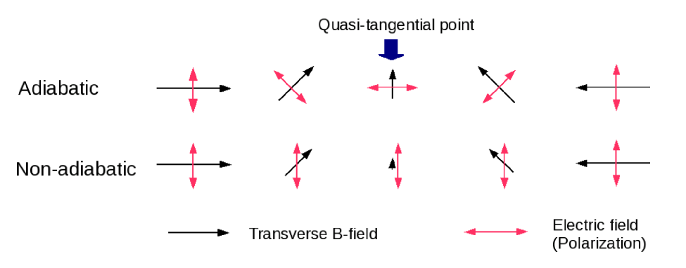
Figure 1: A sketch of the polarization mode evolution across the quasi-tangential point in the adiabatic (upper panels) and non-adiabatic (lower panels) limits. In both cases, the photon polarization vector $\mn@boldsymbol{E}$ (double-arrowed bars) and the transverse magnetic component of the magnetic field $\mn@boldsymbol{B}_{\perp}$ (single-arrowed bars) are shown at five different positions along the ray (from left to right): before, slightly before, at, slightly after, after the QT point. In both limiting cases, there is no net change in the linear polarization when the photon traverses the QT region. Polarization change occurs only in the intermediate cases ($\Gamma_{\rm t}\sim 1$; see text).

Before and after the QT point (where $s=0$), when $|s|\gg\epsilon{\cal R}$, the adiabaticity parameter $\Gamma_{\rm ad}$ increases rapidly with $|s|$ and the mode evolution is generally adiabatic ($\Gamma_{\rm ad}\gg 1$). However at the QT point, $\Gamma_{\rm ad}$ reaches its minimum value:

$$\Gamma_{\rm t}\simeq 1.0\times 10^{8}E_{1}B_{13}^{2}\epsilon^{3}{\cal R}_{1}.$$ (3.22)

The value of $\Gamma_{\rm t}$ determines the mode evolution characteristics across the QT region. Figure 1 shows the qualitative behaviors in two limiting cases: the adiabatic limit ($\Gamma_{\rm t}\gg 1$) and the non-adiabatic limit ($\Gamma_{\rm t}\ll 1$). In the adiabatic case, the photon polarization direction follows the variation of the transverse magnetic field $\mn@boldsymbol{B}_{\perp}$. Since the final direction of $\mn@boldsymbol{B}_{\perp}$ is opposite to the initial direction, the final polarization direction is the same as the initial one. In the non-adiabatic case, $\varphi_{B}$ changes rapidly, so that the polarization direction cannot follow $\mn@boldsymbol{B}_{\perp}$ and remains constant across the QT region. Thus, in both limiting cases, the polarization direction is unchanged when the photon traverses the QT point.

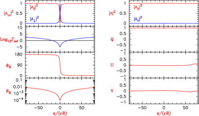
Figure 2: Evolution of photon polarization across the quasi-tangential region for the $\Gamma_{\rm t}\ll 1$ case. The parameters $\epsilon,~{}{\cal R}$ are defined in equation (3.17), $s$ is the distance along the ray ($s=0$ corresponds to the QT point). Prior to the QT point, the photon is assumed to be in the $\parallel$-mode, with $A_{\parallel}=1$ and $A_{\perp}=0$. The angles $\theta_{B},~{}\varphi_{B}$ specify the magnetic field orientation, $A_{X}$ and $A_{Y}$ are the photon polarization amplitudes along the fixed $X,~{}Y$ axis, $Q,~{}U,~{}V$ are the Stokes parameters. For this example, the parameters are $B=10^{12}$ G, $E=1$ keV, $\epsilon=5\times 10^{-5}$, ${\cal R}=100$ km. Note that at the QT point, $\theta_{B}\sim 0$, $\varphi_{B}$ varies rapidly, giving rise to non-adiabatic mode evolution.

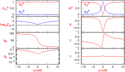
Figure 3: Same as in Fig. 2, except for the $\Gamma_{\rm t}\gg 1$ case, with $\epsilon=10^{-2}$. Note that in this case, at the QT point $\theta_{B}$ is not so close to $0$ and $\varphi_{B}$ varies slowly, giving rise to adiabatic mode evolution.

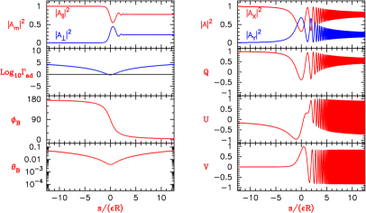
Figure 4: Same as in Fig. 2, except for the $\Gamma_{\rm t}\sim 1$ case, with $\epsilon=4\times 10^{-3}$. Note that in this case, partial mode conversion occurs at the QT point, and the oscillatory behaviors in the Stokes parameters are the result of interference between the two photon modes.

Obviously, a non-trivial change of photon polarization across the QT point occurs only in the intermediate case, $\Gamma_{\rm t}\sim 1$. To obtain the quantitative behaviors of the polarization evolution for general values of $\Gamma_{\rm t}$, we integrate eq. (2.11) numerically. Figures 2 – 4 show three examples of single photon mode evolution in the QT region, corresponding to $\Gamma_{\rm t}\ll 1$, $\Gamma_{\rm t}\gg 1$ and $\Gamma_{\rm t}\sim 1$, respectively. For the $\Gamma_{\rm t}\ll 1$ (non-adiabatic) case (Fig. 2), the photon polarizations (Stokes parameters) are constant throughout the region. For the $\Gamma_{\rm t}\gg 1$ (adiabatic) case (Fig. 3), the photon polarizations (Stokes parameters) change around the QT region, following the variation of $\mn@boldsymbol{B}$, but the final polarizations are very close to the initial values. The most interesting case occurs for $\Gamma_{\rm t}\sim 1$ (Fig. 4). In this intermediate regime, partial mode conversion takes place, so that after crossing the QT point, the photon becomes a mixture of two modes (even when it is in a pure mode prior to QT crossing). The polarization state of the photon is therefore significantly changed by the QT effect.

Based on the above results, we can use $\Gamma_{\rm t}\mathrel{\raise 1.29167pt\hbox{$<$}\mkern-14.0mu\lower 2.58334pt\hbox{$\sim$}}1$ to define the parameter regime for which propagation through the QT region gives rise to an appreciable change in the photon polarization,

$$\epsilon\mathrel{\raise 1.29167pt\hbox{$<$}\mkern-14.0mu\lower 2.58334pt\hbox{$\sim$}}\epsilon_{\rm crit}=2.15\times 10^{-3}(E_{1}B_{13}^{2}{\cal R}_{1})^{-1/3}.$$ (3.23)

Note that when $\epsilon\ll\epsilon_{\rm crit}$, the QT effect is also negligible. This equation effectively maps out the domain where the QT propagation effect must be carefully considered. Outside this domain, one can ignore the QT effect in determining the final observed polarization signals. To translate this effective parameter domain into the physical size of the emission region requires a knowledge of the global NS magnetic field structure. The smallness of $\epsilon_{\rm crit}$ for typical parameters (e.g., $E_{1}\sim 1,~{}B_{13}\sim 1$ and ${\cal R}_{1}\sim 1$) indicates that the “affected” region is a small fraction of the NS surface. But as far as the observed polarization signals are concerned, it is more relevant to compare the size of the “affected” region to the size of the photon emission area. We consider the special case of dipole magnetic field in the next section.

4 Quasi-Tangential Effect in Dipole Magnetic Field

In this section we assume that the NS has a pure dipole field. We focus on X-ray emission from the polar cap region of the star (sections 4.2-4.3), but also consider more general emission regions on the NS surface (section 4.4).

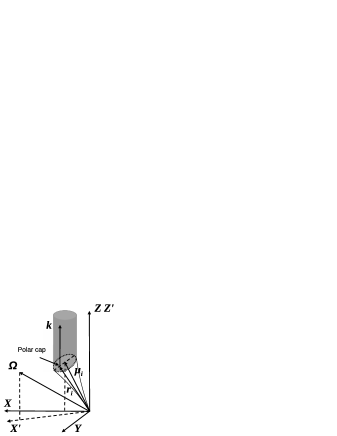
(a)	(b)

Figure 5: Geometrical model of X-ray emission in a dipole magnetic field. Photons are emitted from the polar cap region and propagate toward the observer in the direction ${\mn@boldsymbol{k}}$ along the $Z$ or $Z^{\prime}$-axis. At the time of emission, the magnetic dipole vector is ${\mn@boldsymbol{\mu}_{\rm i}}$ and the initial photon position is ${\bf r}_{\rm i}$. Three coordinate systems are defined: (i) The fixed frame $XYZ$ with $\hat{\mn@boldsymbol{Z}}\parallel\hat{\mn@boldsymbol{k}}$, ${\mn@boldsymbol{\mu}_{\rm i}}$ in the $XZ$-plane and ${\mn@boldsymbol{\mu}_{\rm i}}=\mu(\sin\theta_{\mu_{\rm i}},0,\cos\theta_{\mu_{\rm i}})$; (ii) the fixed frame $X^{\prime}Y^{\prime}Z^{\prime}$ with $\hat{\mn@boldsymbol{Z}}^{\prime}\parallel{\mn@boldsymbol{k}}$, $\hat{\mn@boldsymbol{\Omega}}$ in the $X^{\prime}Z^{\prime}$-plane and $\hat{\mn@boldsymbol{k}}\times\hat{\mn@boldsymbol{\Omega}}=\sin\zeta\,\hat{\mn@boldsymbol{Y}}^{\prime}$; (iii) the instantaneous frame $xyz$, with $\hat{\mn@boldsymbol{z}}\parallel\hat{\mn@boldsymbol{k}}$, $\mn@boldsymbol{B}$ in the $xz$-plane and $\hat{\mn@boldsymbol{k}}\times\hat{\mn@boldsymbol{B}}=-\sin\theta_{B}\hat{\mn@boldsymbol{y}}$. Note that as the photon propagates, the magnetic field it “sees” changes and thus the $xyz$ frame rotates around the $Z$-axis.

4.1 Magnetosphere Field Geometry Along the Ray

To calculate the observed polarized radiation signals, we set up a fixed coordinate system $X^{\prime}Y^{\prime}Z^{\prime}$ with the $Z^{\prime}$-axis along the line-of-sight (pointing from the NS toward the observer) and the $X^{\prime}$-axis in the plane spanned by the $Z^{\prime}$-axis and $\mn@boldsymbol{\Omega}$ (the spin angular velocity vector) (see Fig. 5). The angle between $\mn@boldsymbol{\Omega}$ and ${\mn@boldsymbol{k}}$ is $\zeta$. The magnetic dipole $\mn@boldsymbol{\mu}$ rotates around $\mn@boldsymbol{\Omega}$, and $\alpha$ is the angle between $\mn@boldsymbol{\Omega}$ and $\mn@boldsymbol{\mu}$.

Consider a photon emitted at time $t_{\rm i}$ (corresponding to the NS rotation phase $\Psi_{\rm i}$) from the position $\mn@boldsymbol{r}_{\rm i}=(R_{\ast},\theta_{r_{\rm i}},\varphi_{r_{\rm i}})$ on the NS surface. At this emission time, the magnetic dipole moment is $\mn@boldsymbol{\mu}_{\rm i}$. As the photon propagates along the $Z$-axis, its position vector changes as

$$\mn@boldsymbol{r}=\mn@boldsymbol{r}_{\rm i}+s\hat{\mn@boldsymbol{Z}},$$ (4.24)

where $s=c(t-t_{\rm i})$ is the photon displacement from the emission point. In the meantime, $\mn@boldsymbol{\mu}$ rotates around $\mn@boldsymbol{\Omega}$, and changes according to

$$\mn@boldsymbol{\mu}(s)=\mu\left[(\sin\zeta\cos\alpha+\cos\zeta\sin\alpha\cos\Psi)\hat{\mn@boldsymbol{X}}^{\prime}+\sin\alpha\sin\Psi\hat{\mn@boldsymbol{Y}}^{\prime}+(\cos\zeta\cos\alpha-\sin\zeta\sin\alpha\cos\Psi)\hat{\mn@boldsymbol{Z}}^{\prime}\right],$$ (4.25)

where the rotation phase $\Psi$ is (we set $\Psi=0$ when $\mn@boldsymbol{\mu}$ lies in the $X^{\prime}Z^{\prime}$ plane)

$$\Psi(s)=\Psi_{\rm i}+\Omega(t-t_{\rm i})=\Psi_{\rm i}+s/r_{\rm lc},$$ (4.26)

with $r_{\rm lc}=c/\Omega$ the radius of the light cylinder. The polar angles $(\theta_{\mu}$, $\varphi_{\mu})$ of $\mn@boldsymbol{\mu}$ in the $X^{\prime}Y^{\prime}Z^{\prime}$ frame are given by

$$\cos\theta_{\mu}=\cos\zeta\cos\alpha-\sin\zeta\sin\alpha\cos\Psi,\quad\tan\varphi_{\mu}=\frac{\sin\alpha\sin\Psi}{\sin\zeta\cos\alpha+\cos\zeta\sin\alpha\cos\Psi}.$$ (4.27)

(Similar expressions hold for the polar angles of $\mn@boldsymbol{\mu}_{\rm i}$, $\theta_{\mu_{\rm i}}$ and $\varphi_{\mu_{\rm i}}$, with $\Psi$ replaced by $\Psi_{\rm i}$.) The changing magnetic field as “seen” by the photon is obtained from

$$\mn@boldsymbol{B}(s)=-\nabla(\mn@boldsymbol{\mu}\cdot\mn@boldsymbol{r}/r^{3})=-\frac{\mn@boldsymbol{\mu}}{r^{3}}+\frac{3\mn@boldsymbol{r}}{r^{5}}(\mn@boldsymbol{\mu}\cdot\mn@boldsymbol{r}).$$ (4.28)

When discussing the polarization result of a given rotation phase (at emission) $\Psi_{\rm i}$, it is convenient to introduce another fixed coordinate system $XYZ$ (see Fig. 5), such that $\hat{\mn@boldsymbol{Z}}\parallel\hat{\mn@boldsymbol{k}}$ and ${\mn@boldsymbol{\mu}_{\rm i}}$ in the $XZ$-plane with ${\mn@boldsymbol{\mu}_{\rm i}}=\mu(\sin\theta_{\mu_{\rm i}},0,\cos\theta_{\mu_{\rm i}})$. In the $XYZ$ frame, $\varphi_{\mu_{\rm i}}$ is given by

$$\mn@boldsymbol{\mu}(s)=\mu\left[\sin\theta_{\mu}\cos(\varphi_{\mu}-\varphi_{\mu_{\rm i}})\hat{\mn@boldsymbol{X}}+\sin\theta_{\mu}\sin(\varphi_{\mu}-\varphi_{\mu_{\rm i}})\hat{\mn@boldsymbol{Y}}+\cos\theta_{\mu}\hat{\mn@boldsymbol{Z}}\right].$$ (4.29)

The magnetic field (4.28) as “seen” by the photon is inclined at an angle $\theta_{B}$ with respect to the line-of-sight, and makes an azimuthal angle $\varphi_{B}$ in the $XY$-plane. The angle $\theta_{B}$, $\varphi_{B}$ can be obtained from equation 4.28 via:

$$\cos\theta_{B}(s)=\frac{B_{Z}}{B},\quad\tan\varphi_{B}(s)=\frac{B_{Y}}{B_{X}}.$$ (4.30)

4.2 Polarization Map of the Polar Cap Emission

The observed polarized radiation is the incoherent sum of photons from the emission region on the NS surface. For each emission point, $\mn@boldsymbol{r}_{\rm i}=(R_{\ast},~{}\theta_{r_{\rm i}},~{}\varphi_{r_{\rm i}})$, we integrate the mode evolution equation (2.11) along the photon ray from $\mn@boldsymbol{r}_{\rm i}$ to a large radius, beyond the polarization limiting radius, to determine the final polarization state of the photon. The polarization limiting radius, $r_{\rm pl}$, is where the two photon modes start recoupling to each other, and is determined by the condition $(\omega/c)\Delta n=2|d\varphi_{B}/ds|$. At large distance ($r\gg R_{\ast}$), the magnetic field is simply $\mn@boldsymbol{B}\simeq\left(2\mu_{Z}{\hat{Z}}-\mu_{X}{\hat{X}}-\mu_{Y}{\hat{Y}}\right)/r^{3}$, and $r_{\rm pl}$ is given by

$${r_{\rm pl}\over R_{\ast}}\simeq 70\left(E_{1}B_{\ast 13}^{2}P_{1}\right)^{1/6},$$ (4.31)

where $B_{\ast 13}$ is the polar magnetic field at the stellar surface in units of $10^{13}$ G (see van Adelsberg & Lai 2006 for a more detailed expression). Beyond $r_{\rm pl}$, the photon polarization state is frozen. As mentioned in section 1, the calculations presented in van Adelsberg & Lai (2006) and Lai & Ho (2003b) did not consider the possibility that the photon polarization may change appreciably when crossing the QT point, which typically lies at a much smaller radius than $r_{\rm pl}$.

In general, the radiation emerging from the NS atmosphere at $\mn@boldsymbol{r}_{\rm i}$ includes both the $\parallel$-mode and the $\perp$-mode, with the intensities $I_{\parallel},~{}I_{\perp}$ depending on the field strength, photon energy and emission angle (see Lai & Ho 2003b and van Adelsberg & Lai 2006). In the absence of the QT effect, the radiation at $r>r_{\rm pl}$ will consist of approximately the same $I_{\parallel}$ and $I_{\perp}$, with a small mixture of circular polarization generated around $r_{\rm pl}$ (see van Adelsberg & Lai 2006). This simple result should be modified if there is a significant polarization change when the photon crosses the QT region. Since we are interested in understanding the QT effect, in the following we will assume that at the emission point the radiation is in the $\parallel$-mode, with $I_{\parallel}=1$ and $I_{\perp}=0$.

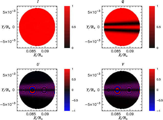
Figure 6: Two-dimensional polarization map of emission from the polar cap region of a NS. The QT propagation effect changes the photon polarization in two narrow bands (confirmed to $-W_{\rm t}/2<Y<W_{\rm t}/2$; see Fig. 7). The input parameters are: $B_{\ast}=10^{14}\,$G, $E=1\,$keV and $\theta_{\mu_{\rm i}}=5^{o}$ (We choose $P=5\,$s, $\alpha=30^{o}$, $\zeta=35^{o}$ and $\Psi_{\rm i}=180^{o}$, although the map depends very weakly on these parameters as long as $\theta_{\mu_{\rm i}}$ is the same).

Figure 7: One-dimensional polarization profiles for emission from the polar cap region of a NS. These profiles are produced by fixing $\theta_{r_{\rm i}}$ while varying $\varphi_{r_{\rm i}}$ of the emission point. The coordinates $XY$ are the projection of the emission point $\mn@boldsymbol{r}_{\rm i}$ on the $XY$ plane (see Fig. 5). The three columns (from left to right) correspond to a fixed $\theta_{r_{\rm i}}=4.8^{o}$, $5.0^{o}$, $5.2^{o}$ (or $X/R_{\ast}\simeq 0.837$, 0.872, 0.906), respectively. In each column, the final Stokes parameters $Q,~{}U,~{}V$ are plotted as a function of $Y$, as well as $\Gamma_{\rm t}$, the adiabaticity parameter at the QT point. The polarizations of photons emitted from the region $-W_{\rm t}/2<Y<W_{\rm t}/2$ (between the two vertical dashed lines, defined by $\Gamma_{\rm t}=3$) are modified by the QT effect. The input parameters for these profiles are: $B_{\ast}=10^{14}\,$G, $E=1\,$keV and $\theta_{\mu_{\rm i}}=5.0^{o}$ (We choose $P=5\,$s, $\alpha=30^{o}$, $\zeta=35^{o}$, $\Psi_{\rm i}=180^{o}$, although the profiles depend very weakly on these parameters as long as $\theta_{\mu_{\rm i}}$ is the same).

Figure 8: Same as Fig. 7, except for $B_{\ast}=10^{14}$ G (the left panels) and $B_{\ast}=4\times 10^{13}$ G (the right panels), both for $P=1$ s.

Figure 6 gives an example of the 2-dimensional polarization map of the final Stokes parameters of photons emitted from the NS polar cap region. This map is produced for a specific set of parameters: surface magnetic field $B_{\ast}$, photon energy $E$, and the angle between ${\mn@boldsymbol{\mu}_{\rm i}}$ and ${\mn@boldsymbol{k}}$, $\theta_{\mu_{\rm i}}$. [For a rotating NS, the map also depends on the angles $\alpha$, $\zeta$, the rotation period $P$ and emission phase $\Psi_{\rm i}$, but the dependence is mainly through $\theta_{\mu_{\rm i}}$ — see eq. (4.27). see below.] Without the QT effect, the final polarization from the polar cap region will be $Q=1$. We see from Fig. 6 that the QT effect gives rise to fine features (with length scale much less than the polar cap size) in the polarization map. In particular, there are two narrow bands (which are parallel to the projected magnetic dipole axis) in the emission region, where the linear polarization $Q$ is significantly reduced because the original $\parallel$ mode is converted across the QT region into a mixture of $\parallel$-mode and $\perp$-mode. In these two narrow belts, non-zero pattens of Stokes $U$ and $V$ are produced. However, these $U,~{}V$ patterns are anti-symmetric with respect to the $Y=0$ line (i.e., the ${\mn@boldsymbol{k}}$-${\mn@boldsymbol{\mu}_{\rm i}}$ plane), so that the observed values of $U$ and $V$ almost equal zero when photons from the whole emission region are added.

In Fig. 7 we show three sections of Fig. 6 along the $Y$-axis for a fixed value of $X$ [$X/R_{\ast}=0.0837$ or $\theta_{r_{\rm i}}=4.8^{o}$ for panel (a), $X/R_{\ast}=0.0872$ or $\theta_{r_{\rm i}}=\theta_{\mu_{\rm i}}=5^{o}$ for panel (b), and $X/R_{\ast}=0.0906$ or $\theta_{r_{\rm i}}=5.2^{o}$ for panel (c)]. We also plot the adiabaticity parameter $\Gamma_{\rm t}$ at the QT point for the photon rays from each emission point. The $\Gamma_{\rm t}$ profile is useful for understanding the results for the Stokes parameters. As the analysis in section 3 shows, photon propagation through the QT region changes the photon polarization significantly only when $\Gamma_{\rm t}\sim 1$. From Fig. 7, we see that the photon Stokes parameters are modified by the QT effect only in two narrow bands, confined in the region $-W_{\rm t}/2<Y<W_{\rm t}/2$, with the boundaries defined approximately by $\Gamma_{\rm t}=3$ (the two vertical dotted lines). Outside this region, $\Gamma_{\rm t}\gg 1$, the mode evolution is adiabatic around the QT point, so that the photon polarization state follows the magnetic field direction and the Stokes parameters are unchanged across the QT region. In the middle of the band (i.e., around $Y=0$), $\Gamma_{\rm t}\ll 1$, mode evolution is non-adiabatic, and the photon polarization state also doesn’t change across the QT point (see Fig. 1).

Figure 8 depicts other examples of the 1D polarization map for different values of stellar magnetic field $B_{\ast}$ ($10^{14}$ and $4\times 10^{13}$ G) and spin period $P$. As in Fig. 7, we see that the final photon polarizations are determined by the value of $\Gamma_{\rm t}$, the QT effective region is confined to $-W_{\rm t}/2<Y<W_{\rm t}/2$ defined by $\Gamma_{\rm t}<3$ (the region between the two vertical dotted lines).

A careful examination of Figs. 7 – 8 shows that due to the NS rotation, the $\Gamma_{\rm t}$ profile and Stokes profiles shift in $Y$ by the amount $\Delta Y\simeq(R_{\ast}\sin\alpha/r_{\rm lc})s_{\rm t}$, where $s_{\rm t}$ is the distance of the QT point from the emission point. Since typically $s_{\rm t}$ is less than a few NS radii, this shift $\Delta Y$ is negligible. According to eq. (3.22), $\Gamma_{\rm t}$ is proportional to $EB_{\ast}^{2}$, thus for smaller $B_{\ast}$ (and smaller $E$) the effective width $W_{\rm t}$ is larger, as seen in Fig. 8. In Fig. 9 we show how $W_{\rm t}$ changes with varying $EB_{\ast}^{2}$. Our numerical result for $W_{\rm t}$ can be fitted by

$$\frac{W_{\rm t}}{R_{\ast}}\simeq 2.7\times 10^{-2}\,(B_{\ast 13}^{2}E_{1})^{-1/3}f(\theta_{\mu_{\rm i}}).$$ (4.32)

Here $f(\theta_{\mu_{\rm i}})$ is a dimensionless function of $\theta_{\mu_{\rm i}}$ [which in turn depends on $\alpha$, $\zeta$ and $\Psi_{\rm i}$, see eq.(4.27)]: $f(\theta_{\mu_{\rm i}}=5^{o})=1$ and varies from 1 to 1.7 for different values of $\theta_{\mu_{\rm i}}$ (see Fig. 10). The scaling relation in eq. (4.32) is derived in the appendix.

Note that the polar cap width (diameter) is given by

$${W_{\rm cap}\over R_{\ast}}=2\sqrt{\frac{R_{\ast}}{c/\Omega}}\simeq 1.3\times 10^{-2}P_{5}^{-1/2},$$ (4.33)

where $P_{5}=P/(5{\rm s})$. Then we have

$$\frac{W_{\rm t}}{W_{\rm cap}}=2.1(B_{\ast 13}^{2}E_{1}P_{5}^{-3/2})^{-1/3}f(\theta_{\mu_{\rm i}}).$$ (4.34)

Equation (4.34) implies that the size of the effective QT region (where the QT effect changes the photon polarization) can be comparable to the polar cap size for some parameters (e.g., low photon energy and low magnetic field strength).

Figure 9: The width of the QT effective region $-W_{\rm t}/2<Y<W_{\rm t}/2$, defined by $\Gamma_{\rm t}<3$, as a function of the surface magnetic field strength and photon energy. Here $B_{\ast 14}=B_{\ast}/(10^{14}\,\rm G)$, $E_{1}=E/(1\,\rm keV)$. The different lines correspond to different $\theta_{\mu_{\rm i}}$: $\theta_{\mu_{\rm i}}=5^{o}$ (solid line), $\theta_{\mu_{\rm i}}=15^{o}$ (dashed line), $\theta_{\mu_{\rm i}}=45^{o}$ (dot-dashed line).

Figure 10: The dimensionless function $f(\theta_{\mu_{\rm i}})$, as defined in eq. (4.32).

4.3 Quasi-Tangential Effect on the Observed Polarization

As discussed above, when linearly polarized radiation with $Q=I=1$ traverses the QT region with $\Gamma_{\rm t}<3$, its Stokes parameters will be changed (so that $Q$ will become less than unity, and $U,~{}V$ will be nonzero; see Figs. 7 – 8). However, when adding up radiation from a finite emission region, we find $\int dYU\simeq 0$ and $\int dYV\simeq 0$. Thus the net effect of the QT propagation is to reduce the degree of the linear polarization of the photon. In general, if $F_{Q}$ is the flux of linearly polarized radiation prior to passing the QT region, then after traversing the QT region, the linearly polarized radiation flux $\bar{F_{Q}}$ can be obtained by

$${\bar{F_{Q}}\over F_{Q}}=\int_{|Y|<W_{\rm em}/2}\frac{Q(Y)}{I}{\rm d}Y,$$ (4.35)

where $W_{\rm em}$ is the width of the emission region. As seen in section 4.2 (see Figs. 7 – 8), the $Q(Y)$ profiles for different parameters are similar, so that $\bar{F_{Q}}/F_{Q}$ depends only on $W_{\rm t}/W_{\rm em}$. Our numerical result for $\bar{F_{Q}}/F_{Q}$ as a function of $W_{\rm t}/W_{\rm em}$ is shown in Fig. 11. For a given set of parameters ($B_{\ast}$, $E$, $\theta_{\mu_{\rm i}}$), we can use eq. (4.32) and Fig. 10 to obtain $W_{\rm t}$, and then use Fig. 11 to read off the ratio $\bar{F_{Q}}/F_{Q}$. If $W_{\rm t}\mathrel{\raise 1.29167pt\hbox{$<$}\mkern-14.0mu\lower 2.58334pt\hbox{$\sim$}}W_{\rm em}$, we find that $\bar{F_{Q}}/F_{Q}$ is approximately given by

$$\bar{F_{Q}}/F_{Q}\simeq 1-\frac{W_{\rm t}}{2.5W_{\rm em}}\qquad({\rm for}~{}~{}W_{\rm t}/W_{\rm em}\mathrel{\raise 1.29167pt\hbox{$<$}\mkern-14.0mu\lower 2.58334pt\hbox{$\sim$}}1).$$ (4.36)

Note that for $W_{\rm t}\ll W_{\rm em}$, the effective QT region is much smaller compared to the emission region so that $\bar{F_{Q}}/F_{Q}\simeq 1$; for $W_{\rm em}\ll W_{\rm t}$, the photon mode evolution across the QT region is non-adiabatic so that $\bar{F_{Q}}/F_{Q}$ is also close to unity. Thus in both $W_{\rm t}/W\ll 1$ and $W_{\rm t}/W_{\rm em}\gg 1$ limits, $\bar{F_{Q}}/F_{Q}=1$, i.e., the linear polarization is unchanged by the QT effect. The minimum value of $\bar{F_{Q}}/F_{Q}$ occurs at $W_{\rm t}/W_{\rm em}\simeq 1.8$.

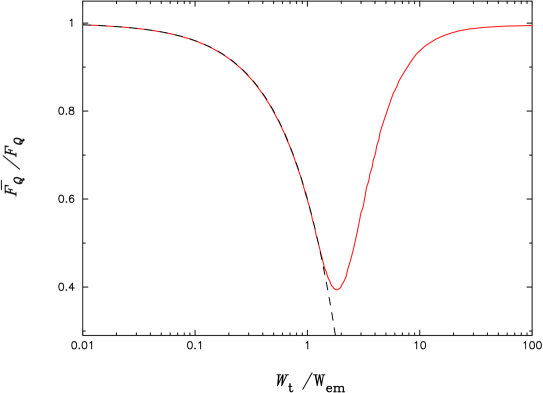
Figure 11: The effect of QT propagation on the observed linear polarization: $F_{Q}$ ($\bar{F_{Q}}$) is the linearly polarized radiation flux before (after) traversing the QT region; see eq. (4.35). Here $W_{\rm t}$ is the width of the effective QT region (where $\Gamma_{\rm t}<3$) and $W_{\rm em}$ is the width of the emission region. For $W_{\rm t}/W_{\rm em}\mathrel{\raise 1.29167pt\hbox{$<$}\mkern-14.0mu\lower 2.58334pt\hbox{$\sim$}}1$, $\bar{F_{Q}}/F_{Q}$ can be approximated by eq. (4.36), which is shown as the dashed line.

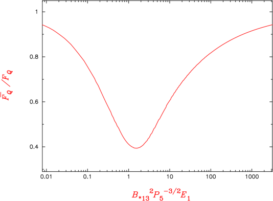
Figure 12: The reduction factor $\bar{F_{Q}}/F_{Q}$ of the linear polarization as a function of the photon energy (and other parameters). Here $B_{\ast 13}=B_{\ast}/(10^{13}\,\rm G)$, $E_{1}=E/(1\rm\,keV)$, $P_{5}=P/(5\,\rm s)$, and we have assumed $W_{\rm em}=W_{\rm cap}$. The angle between ${\mn@boldsymbol{k}}$ and ${\mn@boldsymbol{\mu}_{\rm i}}$ is chosen to be $\theta_{{\mu_{\rm i}}}=5^{o}$.

Suppose the emission is coming from polar cap region with width $W_{\rm em}=W_{\rm cap}$, then according to eq. (4.34), $W_{\rm t}/W_{\rm cap}$ is proportional to $(B_{\ast 13}^{2}E_{1})^{-1/3}P_{5}^{1/2}$. Thus, for given $B_{\ast 13}$, $P_{5}$ and $\theta_{\mu_{\rm i}}$, we can translate Fig. 11 into a spectrum for $\bar{F_{Q}}/F_{Q}$ — This spectrum is shown in Fig. 12. We see that at sufficiently low energies and high energies, $\bar{F_{Q}}/F_{Q}\simeq 1$, and the minimum reduction of the degree of linear polarization due to the QT effect occurs at $W_{\rm t}/W_{\rm cap}\simeq 1.8$, corresponding to the photon energy

$$E_{\rm min}\simeq 1.6B_{\ast 13}^{-2}P_{5}^{3/2}f^{3}(\theta_{\mu_{\rm i}})\,{\rm keV}.$$ (4.37)

Now we consider the (energy-dependent) polarization light curve produced by the polar cap emission of a rotating NS. As the NS rotates, the ${\mn@boldsymbol{k}}$-${\mn@boldsymbol{\mu}_{\rm i}}$ angle $\theta_{\mu_{\rm i}}$ changes with the rotation phase $\Psi_{\rm i}$ [see eq. (4.27)]. According to eq. (4.34) and Figs. 10, 11, different $\theta_{\mu_{\rm i}}$ will give different $\bar{F_{Q}}/F_{Q}$ , which means $\bar{F_{Q}}/F_{Q}$ will evolve with the rotation phase $\Psi_{\rm i}$. Moreover, $W_{\rm t}/W_{\rm cap}$ and $\bar{F_{Q}}/F_{Q}$ depend on the photon energy. Figs. 13 and 14 present two examples of the phase evolution of $W_{\rm t}/W_{\rm cap}$ and $\bar{F_{Q}}/F_{Q}$, for $B_{\ast}=10^{13}$ G and $10^{14}$ G, respectively. As noted before, $\bar{F_{Q}}/F_{Q}$ reaches a minimum at $W_{\rm t}/W_{\rm cap}=1.8$ (see Fig. 11). In the case depicted in Fig. 13, $W_{\rm t}/W_{\rm cap}>1.8$ for $E=1$ keV and 0.5 keV at all phases, thus $\bar{F_{Q}}/F_{Q}$ is larger for lower photon energies (since $W_{\rm t}/W_{\rm cap}$ increases with $E$). In Fig. 14, $W_{\rm t}/W_{\rm cap}<1.8$ for all the three photon energies ($E=0.5,~{}1,~{}5$ keV), so that $\bar{F_{Q}}/F_{Q}$ is larger for higher energies.

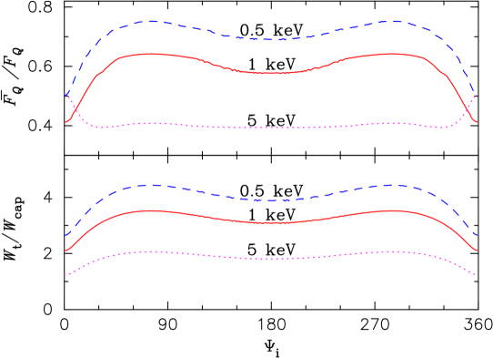
Figure 13: The phase evolution of the modification of linear polarization by the QT effect, $F_{Q}^{\prime}/F_{Q}$ (upper panel) and the effective QT region width relative to the polar cap size, $W/W_{\rm cap}$ (lower panel). The different curves are for different photon energies: $E=$0.5 keV (dashed lines), 1 keV (solid lines) and 5 keV (dotted line). The input model parameters are: $B_{\ast}=10^{13}$ G, $P=5$ s, $\alpha=30^{o}$ and $\zeta=35^{o}$. The emission region size is assumed to be $W_{\rm cap}$.

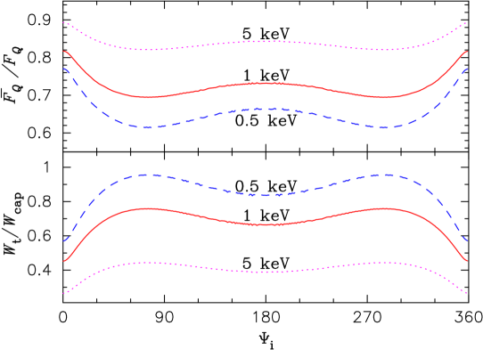
Figure 14: Same as Fig. 13, except for $B_{\ast}=10^{14}$ G.

To produce the observed polarized radiation fluxes, using the results present above, we will need input $F_{Q}$. In general, the emergent radiation from the NS atmosphere (before passing through the QT region) is linearly polarized, with $F_{Q}$ dependent on $E$ and the rotation phase (and $B_{\ast}$ $\alpha$, $\zeta$). In the $XYZ$ frame, the radiation has polarized fluxes $F_{Q}\neq 0$ (which can be either positive or negative), $F_{U}=0$ and $F_{V}=0$. Using $F_{Q}$ from an atmosphere model and our result for $\bar{F_{Q}}/F_{Q}$, we can compute ${\bar{F}}_{Q}$, the polarized flux after passing through the QT region. Then the observed polarized radiation fluxes in the fixed $X^{\prime}Y^{\prime}Z^{\prime}$ frame are given by

$$F_{Q}^{\prime}={\bar{F}}_{Q}\cos 2\varphi_{B}(r_{\rm pl}),\quad F_{U}^{\prime}={\bar{F}}_{Q}\sin 2\varphi_{B}(r_{\rm pl}),$$ (4.38)

where $\varphi_{B}(r_{\rm pl})$ is the azimuthal angle of the magnetic field, $\varphi_{B}$, evaluated at the polarization limiting radius $r=r_{\rm pl}$. For $r_{\rm pl}\ll r_{\rm lc}=c/\Omega$, or for spin frequency $\ll 70$ Hz, $\varphi_{B}(r_{\rm pl})\simeq\pi+\varphi_{\mu}\simeq\pi+\varphi_{\mu_{\rm i}}$ (see Lai & Ho 2003b; van Adelsberg & Lai 2006), thus $F_{Q}^{\prime}=\bar{F_{Q}}\cos 2\varphi_{\mu_{\rm i}}$ and $F_{U}^{\prime}=\bar{F_{Q}}\sin 2\varphi_{\mu_{\rm i}}$.

4.4 Quasi-Tangential Effect for Different Emission Regions

In the previous subsections we have focused on emission from the polar cap region of the NS. In reality, the “hot spot” on the NS surface may be larger. The QT effect also exists outside the polar cap region.

As discussed above, the QT effective region is confined to $\Gamma_{\rm t}<3$. For a given dipole field geometry, we can calculate $\Gamma_{\rm t}$ for photon rays emerging from different points on the stellar surface. Figs. 15 and 16 give two examples of the effective QT region as defined by $\Gamma_{\rm t}<3$, for the ${\mn@boldsymbol{k}}$-${\mn@boldsymbol{\mu}_{\rm i}}$ angle $\theta_{\mu_{\rm i}}=15^{o}$ and $5^{o}$, respectively. For each emission point, if we ignore the QT effect, the final photon polarization is dominated by the wave mode coupling effect and the polarization position angle (PA) is approximately determined by $\varphi_{B}$ at polarization limiting radius $r_{\rm pl}$ (again, assuming at emission the photon is in the $\parallel$-mode). Generally we have $R_{\ast}\ll r_{\rm pl}\ll r_{\rm lc}$, so $\varphi_{B}(r_{\rm pl})\simeq\varphi_{\mu_{\rm i}}+\pi$. Therefore, the final polarization direction of the X-ray photon from any point of the star surface are always parallel to the ${\mn@boldsymbol{k}}$-$\mn@boldsymbol{\mu}$ plane. However, in the QT effective region, the final PA may be modified when the photon propagates through QT region (see the lower panel of Fig. 15). Note that the final polarization angles are always symmetric with respect to the ${\mn@boldsymbol{k}}$-$\mn@boldsymbol{\mu}$ plane. Thus, as discussed before, when adding up radiation from a finite emission region, the net effect of QT propagation is to reduce the degree of linear polarization without changing the polarization angle.

Special caution must be taken when $\theta_{\mu_{\rm i}}$ is small. We see from Fig. 16 that for $\theta_{\mu_{\rm i}}=5^{o}$, the effective QT region may cover a significant part of the stellar surface (In Fig. 16, the hatched region only shows the effective QT region that satisfies $\theta_{r_{\rm i}}<20^{o}$.) This can be understood as follows. For $R_{\ast}\ll r\ll r_{\rm lc}$ the transverse parts of the dipole magnetic field are [see eq. (4.28)]

$$B_{X}=\frac{\mu}{r^{3}}\left(-\sin\theta_{\mu_{\rm i}}+3X_{\rm i}\cos\theta_{\mu_{\rm i}}/r\right),\quad B_{Y}=\frac{\mu}{r^{3}}\left(\frac{3Y_{\rm i}\cos\theta_{\mu_{\rm i}}}{r}\right).$$ (4.39)

with $\mn@boldsymbol{r}=\mn@boldsymbol{r}_{\rm i}+s\hat{\mn@boldsymbol{Z}}$ (neglecting light bending) and $s\gg r_{\rm i}$, and $X_{\rm i},~{}Y_{\rm i}$ are the $X,Y$ components of the emission position $\mn@boldsymbol{r}_{\rm i}$. For $\theta_{\mu_{\rm i}}\gg 3R_{\ast}/r$, we have $B_{X}\simeq-(\mu/r^{3})\sin\theta_{\mu_{\rm i}}$, $B_{Y}\simeq 0$, thus outside the QT region, the final polarization is aligned with the ${\mn@boldsymbol{k}}-{\mn@boldsymbol{\mu}_{\rm i}}$ plane. However, for $\theta_{\mu_{\rm i}}\mathrel{\raise 1.29167pt\hbox{$<$}\mkern-14.0mu\lower 2.58334pt\hbox{$\sim$}}3R_{\ast}/r$, we no longer can neglect $B_{Y}$ relative to $B_{X}$. Thus for sufficiently small $\theta_{\mu_{\rm i}}$, polarization alignment will not be achieved for most emission points. Figure 17 shows the 1D profiles of the final $Q$, $U$, $V$ and $\Gamma_{\rm t}$ for a fixed $\theta_{r_{\rm i}}$ and varying $\varphi_{r_{\rm i}}$, all with $\theta_{\mu_{\rm i}}=5^{o}$. In the left and middle panels where $\theta_{r_{\rm i}}=10^{o}$ and $20^{o}$, the profiles are similar to the cases examined before (see Figs. 7 and 8). For the $\theta_{r_{\rm i}}=30^{o}$ case (the right panels of Fig. 17), $\Gamma_{\rm t}$ is always less that 3. The reason is that when $\theta_{r_{\rm i}}$ is large, the QT point lies far away from the star $r_{\rm t}\gg R_{\ast}$ (and it is even possible that $r_{\rm t}>r_{\rm pl}$ for sufficiently large $\theta_{r_{\rm i}}$). In this case (small $\theta_{\mu_{\rm i}}$ and emission from the region far away from the magnetic pole), the simple prescription we have presented in section 4.2 – 4.3 to account for the QT effect cannot be used, and numerical ray integration from each emission point is necessary.

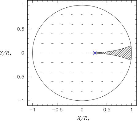
Figure 15: The quasi-tangential effect for X-rays emitted from the whole surface of the NS with the ${\mn@boldsymbol{k}}$-${\mn@boldsymbol{\mu}_{\rm i}}$ angle $\theta_{\mu_{\rm i}}=15^{o}$. Here we use the $XYZ$ frame with $\hat{\mn@boldsymbol{k}}\parallel\hat{\mn@boldsymbol{Z}}$, ${\mn@boldsymbol{\mu}_{\rm i}}$ in $XZ$-plane and the circle corresponds to the project star surface. In the upper panel, the hatched region is the effective QT region, defined by $\Gamma_{\rm t}<3$. The bars show the polarization direction. The cross marks the projected dipole axis ${\mn@boldsymbol{\mu}_{\rm i}}$ on the stellar surface. The lower panel shows the enlarged effective QT region. The other input parameters are: $B_{\ast}=10^{14}$ G, $E=1$ keV.

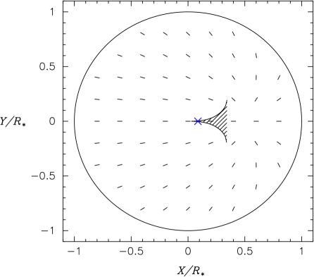
Figure 16: Same as the upper panel of Fig. 15, except with $\theta_{\mu_{\rm i}}=5^{o}$.

Figure 17: Similar to Fig. 7, but for emission from larger regions of the NS. Here we use the varying $\varphi_{r_{\rm i}}$ as the $X$-axis. The three columns (from left to right) correspond to a fixed $\theta_{\mu_{\rm i}}=10^{o},~{}20^{o},~{}30^{o}$ (or $X/R_{\ast}=0.174,~{}0.342,~{}0.5$ at $Y=0$). The input parameters are $B_{\ast}=10^{14}\,$G, $E=1$ keV, $\theta_{\mu_{\rm i}}=5^{o}$.

5 Discussion

We have studied the evolution of photon polarization in a neutron star magnetosphere whose dielectric property is dominated by vacuum birefringence. We have focused on X-rays because of the potential of using X-ray polarimetry to constrain neutron star magnetic fields and to probe strong-field QED (see Heyl & Shaviv 2002; Heyl et al. 2003; Lai & Ho 2003b).

5.1 X-ray Polarization Signals without QT Effect

If one neglects the QT propagation effect studied in this paper, then it is straightforward to obtain the obserevd polarized X-ray fluxes (Stokes parameters) from the fluxes at the emission region, at least approximately, without integrating the polarization evolution equations in the magnetosphere (Lai & Ho 2003b; van Adelsberg & Lai 2006). For a given (small) emission region of projected area $\Delta A_{\perp}$, one need to know the intensities of the two photon modes at emission, $I_{\perp}$ and $I_{\parallel}$. In the case of thermal emission, these can be obtained directly from atmosphere/surface models. As the radiation propagates through the magnetosphere, the photon mode evolves adiabatically, following the variation of the magnetic field, until the polarization limiting radius $r_{\rm pl}$, at which point the polarization is frozen. Thus the polarized radiation flux beyond $r_{\rm pl}$ is $F_{Q}=(I_{\parallel}-I_{\perp})\Delta A_{\perp}/D$, and $F_{U}\simeq F_{V}\simeq 0$, where $D$ is the distance of the source, $F_{Q}$ and $~{}F_{U}$ are defined in the coordinate system such that the stellar magnetic field at $r_{\rm pl}$ lies in the $XZ$ plane (with the $Z$-axis pointing towards the observer). Since $r_{\rm pl}$ is much larger than the stellar radius, the magnetic fields as ”seen” by different photon rays are aligned and are determined by the dipole component of the stellar field, one can simply add up contributions from different surface emission areas to $F_{Q}$ to obtain the observed polarization fluxes.

Note that the description of the polarization evolution in the last paragraph is valid regardless of the possible complexity of the magnetic field near the stellar surface. This opens up the possibility of constraining the surface magnetic field of the neutron star using X-ray polarimetry. For example, the polarization light curve (particularly the dependence on the rotation phase) depends only on the dipole component of the magnetic field, while the intensity lightcurve of the same source depends on the surface magnetic field. On the other hand, the linear polarization spectrum (i.e., its dependence on the photon energy) depends on the magnetic field at the emission region (Lai & Ho 2003b; van Adelsberg 2006); thus it is possible that a NS with a weak dipole field ($\mathrel{\raise 1.29167pt\hbox{$<$}\mkern-14.0mu\lower 2.58334pt\hbox{$\sim$}}7\times 10^{13}$ G) may exhibit X-ray polarization spectrum characteristic of a $B\mathrel{\raise 1.29167pt\hbox{$>$}\mkern-14.0mu\lower 2.58334pt\hbox{$\sim$}}7\times 10^{13}$ G NS (see section 1).

5.2 Effect of QT Propagation

The QT propagation effect studied in this paper complicates the above picture somewhat. When a photon passes through the QT region (which typically lies within a few stellar radii), its polarization modes can be temporarily recoupled, and this can give rise to partial mode conversion. Thus after passing through the QT point, the mode intensities change to ${\bar{I}}_{\parallel}\neq I_{\parallel}$ and ${\bar{I}}_{\perp}\neq I_{\perp}$. The observed polarization flux is then ${\bar{F}}_{Q}=({\bar{I}}_{\parallel}-{\bar{I}}_{\perp})\Delta A/D\neq F_{Q}$.

In the most general situations, to account for the QT propagation effect, it is necessary to integrate the polarization evolution equations (see section 2.2) in order to obtain the observed radiation Stokes parameters. However, we show in this paper that for generic near-surface magnetic fields, the effective region where the QT effect leads to significant polarization changes covers only a small area of the neutron star surface [see section 3, particularly eq. (3.22)]. For a given emission model (and the size of the emission region) and magnetic field structure, one can use our result in section 3 to evaluate the importance of the QT effect. In the case of surface emission from around the polar cap region of a dipole magnetic field, we have quantified the effect of QT propagation in detail (section 4) and provided a simple, easy-to-use prescription to account for the QT effect in determining the observed pollarizatin fluxes. Our key results are presented in sections 4.2 – 4.3, particularly Fig. 11 and equations (4.32) (together with Fig. 10) and (4.35) – (4.36). As discussed in section 4.3, the net effect of QT propagation is to reduce the degree of linear polarization, so that ${\bar{F}}_{Q}/F_{Q}<1$, with the reduction factor depending on the photon energy, magnetic field strength, geometric angles, rotation phase and the emission area. The largest reduction is about a factor of two, and occurs for a particular emission size ($W_{\rm t}/W_{\rm em}\simeq 1.8$; see Fig. 11). Obviously, for emission from a large area of the stellar surface, the QT effect is negligible.

Overall, the QT effect will have a small or at most modest effect on the observed X-ray polarization signals from magnetized neutron stars. Thus the the description of X-ray polarizaton signals given in section 5.1 remains largely valid. In most situations (the exceptions are discussed in section 4.4), the QT effect can be accounted for in a straightforward manner using the result presented in our paper.

Appendix A Derivation of Equation (4.31)

Consider the emission from the polar cap region of a non-rotating NS. In the $XYZ$-frame (see Fig. 5, ${\mn@boldsymbol{k}}\parallel\hat{\mn@boldsymbol{Z}}$, ${\mn@boldsymbol{\mu}_{\rm i}}$ in $XZ$-plane), the initial magnetic momentum is

$${\mn@boldsymbol{\mu}_{\rm i}}=\mu(\sin\theta_{\mu_{\rm i}},0,\cos\theta_{\mu_{\rm i}}),$$ (A.40)

and the photon position is

$$\mn@boldsymbol{r}=(R_{\ast}\sin\theta_{r_{\rm i}},Y,R_{\ast}\cos\theta_{r_{\rm i}}+s),$$ (A.41)

where $s$ is the displacement from the emission point, and $Y\ll R_{\ast}$. We want to evaluate $\Gamma_{\rm t}$ at the QT point $s=s_{\rm t})(Y)$ as a function of $Y$. The magnetic field is given by eq. (4.28), and has components:

$$B_{X} = -\frac{\sin\theta_{\mu_{\rm i}}}{r^{3}}+\frac{3R_{\ast}\sin\theta_{\mu_{\rm i}}}{r^{5}}(R_{\ast}+s\cos\theta_{\mu_{\rm i}}),$$

$$B_{Y} = \frac{3Y}{r^{5}}(R_{\ast}+s\cos\theta_{\mu_{\rm i}}),$$ (A.42)

(here we set $\mu=1$). For a given $Y$, The QT point ($s=s_{\rm t}(Y)$) is defined by

$$\frac{{\rm d}B_{\perp}^{2}}{{\rm d}s}\mid_{r=r_{\rm t}}=0.$$ (A.43)

We can expand $B_{X}$ and $B_{Y}$ near $s=s_{\rm t}(Y)$ using Taylor expansion:

$$B_{X} = B_{X\rm t}+F_{1}\Delta s$$

$$B_{Y} = (H+F_{2}\Delta s)Y$$ (A.44)

with $\Delta s=s-s_{\rm t}$. Note that $B_{X\rm t}$, $H$, $F_{1}$, $F_{2}$ all depend on $s_{\rm t}(Y)$. Substitute eq. (A.44) into eq. (A.43), we have

$$B_{X\rm t}=-Y^{2}\frac{HF_{2}}{F_{1}}.$$ (A.45)

From eq. (A.45) we see that

$$\Delta s_{\rm t}(Y)=s_{\rm t}(0)+{\cal O}(Y^{2}).$$ (A.46)

Thus

$$F_{1}=F_{10}+{\cal O}(Y^{2}),~{}F_{2}=F_{20}+{\cal O}(Y^{2}),~{}H=H_{0}+{\cal O}(Y^{2}),~{}B_{X\rm t}=-Y^{2}\frac{H_{0}F_{20}}{F_{10}}+{\cal O}(Y^{4})$$ (A.47)

where $F_{10}$, $F_{20}$, $H_{0}$ are constants. . The azimuthal angle of $\mn@boldsymbol{B}$ is determined by $\tan\varphi_{B}=B_{Y}/B_{X}$. Therefore $\varphi_{B}^{\prime}$ at $s=s_{\rm t}$ is

$$\varphi_{B}^{\prime}\mid_{s=s_{\rm t}} = \cos^{2}\varphi_{B}\left(\frac{B_{Y}}{B_{X}}\right)^{\prime}\mid_{r=r_{\rm t}}=\frac{YHF_{1}+Y^{3}HF_{2}^{2}/F_{1}}{Y^{2}H^{2}+Y^{4}(HF_{2}/F_{1})^{2}}\propto 1/Y$$ (A.48)

We also have

$$\sin\theta_{B}\mid_{s=s_{\rm t}}=\frac{B_{\perp}}{B}\propto Y$$ (A.49)

Substitute eq. (A.48) and (A.49) into eq. (2.13), the adiabaticity parameter at QT point is then given by

$$\Gamma_{\rm t}\propto B_{\ast}^{2}EY^{3}.$$ (A.50)

The QT effective width $W_{\rm t}$, defined by $\Gamma_{\rm t}=3$, is then $W_{\rm t}\propto(B_{\ast}^{2}E)^{-1/3}$.

References

- [] Adler, S.L. 1971, Ann. Phys., 67, 599
- [] Beloborodov, A. M., 2002, ApJ, 565, 808
- [] Beloborodov, A. M. & Thompson, C., 2006, 36th COSPAR Scientific Assembly. Held 16 - 23 July 2006.
- [] Costa,E., Bellazzini, R., & Bregeon, J. et al. 2008, in “Space Telescopes and Instrumentation 2008: Ultraviolet to Gamma Ray”. Edited by Turner, Martin J. L.; Flanagan, Kathryn A. Proceedings of the SPIE, Volume 7011. arXiv:0810:2700
- [] Daugherty, J. K. & Harding, A. K., 1982, ApJ, 252, 337
- [] Gnedin Yu.N. and Sunyaev R.A., 1974, A&A. 36, 379
- [] Gnedin, Yu.N., Pavlov, G.G., & Shibanov, Yu.A. 1978, Sov. Astron. Lett., 4(3), 117
- [] Harding, A.K., & Lai, D. 2006, Rept. Prog. Phys., 69, 2631
- [] Heyl, J.S. & Hernquist, L. 1997, J. Phys. A, 30, 6485
- [] Heyl, J.S., & Shaviv, N.J. 2002, Phys. Rev. D66, 023002
- [] Heyl, J.S., Shaviv, N.J., & Lloyd, D. 2003, MNRAS, 342, 134
- [] Hibschman, J. A. & Arons, J., 2001, ApJ, 560, 871
- [] Ho, W. C. & Lai, D. 2001, MNRAS, 327, 1081
- [] Ho, W. C. & Lai, D. 2003, MNRAS, 338, 233
- [] Kaplan, D.L. 2008, arXiv:0801.1143
- [] Kaspi, V.M., Roberts, M., & Harding, A.K. 2006, in “Compact Stellar X-ray Sources” eds. W. Lewin & M. van der Klis (Cambridge Univ. Press), p279.
- [] Lai, D. & Ho, W. C. G. 2002, ApJ, 566, 373
- [] Lai, D. & Ho, W. C. G. 2003a, ApJ, 588, 962
- [] Lai, D. & Ho, W. C. 2003b, PhRvL, 91, 1101
- [] Lodenquai, J., Canuto, V., Ruderman, M. & Tsuruta, S. 1974, ApJ, 190, 141
- [] Medin, Z. & Lai, D., 2009, in preparation
- [] Mészáros, P., High-Energy Radiation from Magnetized Neutron Stars, Univ. Chicago Press, Chicago, 1992
- [] Mészáros, P., et al. 1988, ApJ, 324, 1056
- [] Mészáros, P. & Ventura, J. 1979, Phys. Rev. D 19, 3565
- [] Pavlov, G.G. & Gnedin, Yu.N. 1984, Sov. Sci. Rev. E: Astrophys. Space Phys. 3, 197
- [] Pavlov, G.G. & Zavlin, V.E. 2000, ApJ, 529, 1011
- [] Potekhin A.Y. & Chabrier G., 2003, ApJ, 585, 955
- [] Potekhin, A. Y., Lai, D., Chabrier, G., & Ho, W.C.G., 2004, ApJ, 612, 1034
- [] Swank, J., Kallman, T., & Jahoda, K. 2008, presentation at the 37th COSPAR Scientific Assembly, p.3102
- [] Schwinger, J. 1951, Phys. Rev., 82, 664
- [] Thompson, C., Lyutikov, M., & Kulkarni, S. R. 2002, ApJ, 574, 332
- [] van Adelsberg, M. & Lai, D. 2006, MNRAS, 373, 1495
- [] van Kerkwijk, M.H. & Kaplan, D.L. 2007, Ap&SS, 308, 191
- [] Wang, C. & Lai, D. 2007, MNRAS, 377, 1095
- [] Yakovlev, D.G., & Pethick, C.J. 2004, ARAA, 42, 169;