Critical Josephson current through a bistable single-molecule junction

Abstract

We compute the critical Josephson current through a single-molecule junction. As a model for a molecule with a bistable conformational degree of freedom, we study an interacting single-level quantum dot coupled to a two-level system and weakly connected to two superconducting electrodes. We perform a lowest-order perturbative calculation of the critical current and show that it can significantly change due to the two-level system. In particular, the $\pi$-junction behavior, generally present for strong interactions, can be completely suppressed.

I Introduction

The swift progress in molecular electronics achieved during the past decade has mostly been centered around a detailed understanding of charge transport through single-molecule junctions,nitzan ; molel where quantum effects generally turn out to be important. When two superconducting (instead of normal) electrodes with the same chemical potential but a phase difference $\varphi$ are attached to the molecule, the Josephson effectgolubov implies that an equilibrium current $I(\varphi)$ flows through the molecular junction. Over the past decade, experiments have observed gate-tunable Josephson currents through nanoscale junctions, helene ; morpurgo ; reulet ; buit1 ; buit2 ; doh ; kasumov ; jorgensen ; lieber ; leo ; CPR-exp1 ; wernsdorfer ; chauvin ; christian ; nygard ; CPR-exp2 ; landman ; hakonen ; parisbasel including out-of-equilibrium cases, and many different interesting phenomena have been uncovered. In particular, the current-phase relation has been measured by employing a superconducting quantum interference device.CPR-exp1 ; wernsdorfer ; CPR-exp2 For weakly coupled electrodes, the current-phase relation isgolubov

$$I(\varphi)=I_{c}\sin(\varphi),$$ (1)

with the critical current  $I_{c}$.

The above questions have also been addressed by many theoretical works. It has been shown that the repulsive electron-electron (e-e) interaction $U>0$, acting on electrons occupying the relevant molecular level, can have a major influence on the Josephson current.shiba ; glazman ; spivak ; rozhkov ; zachar ; clerk ; matsumoto ; vecino ; siano ; choi ; kroha ; novotny ; meden ; florens For intermediate-to-strong coupling to the electrodes, an interesting interplay between the Kondo effect and superconductivity takes place.glazman ; clerk ; vecino ; siano ; choi ; meden In the present paper, we address the opposite limit where, for sufficiently large $U$, a so-called $\pi$-phase can be realized, with $I_{c}<0$ in Eq. (1). In the $\pi$-regime, $\varphi=\pi$ corresponds to the ground state of the system (or to a minimum of the free energy for finite temperature), in contrast to the usual $0$-state with $I_{c}>0$, where $\varphi=0$ in the ground state.footnew The sign change in $I_{c}$ arises due to the blocking of a direct Cooper pair exchange when $U$ is large. Double occupancy on the molecular level is then forbidden, and the remaining allowed processes generate the sign change in $I_{c}$.shiba ; glazman ; spivak ; zachar ; matsumoto ; novotny The most natural way to explain the $\pi$-junction behavior is by perturbation theory in the tunnel couplings connecting the molecule to the electrodes. Experimental observations of the $\pi$-phase were recently reported for InAs nanowire dotsCPR-exp1 and for nanotubes,wernsdorfer ; tomas1 but a $\pi$-junction is also encountered in superconductor-ferromagnet-superconductor structures.SFS1 ; SFS2 Accordingly, theoretical works have also analyzed spin effects in molecular magnets coupled to superconductors.molmag1 ; molmag2 ; molmag3

The impressive experimental control over supercurrents through molecular junctions reviewed above implies that modifications of the supercurrent due to vibrational modes of the molecule play a significant and observable role.novotny ; bcs-holstein1 ; bcs-holstein2 ; bcs-holstein3 We have recently discussed how a two-level system (TLS) coupled to the dot’s charge is affected by the Josephson current carried by Andreev states.zazuprl For instance, two conformational configurations of a molecule may realize such a TLS degree of freedom. Experimental results for molecular break junctions with normal leads were interpreted using such models, tls-exp1 ; tls-exp2 ; tls-exp3 ; tls-the ; tls-the2 ; fabrizio but the TLS can also be created artifically using a Coulomb-blockaded double dot.zazuprl A detailed motivation for our model, where the Pauli matrix $\sigma_{z}$ in TLS space couples to the dot’s charge, and its experimental relevance has been given in Refs. zazuprl, ; fabrizio, . While our previous workzazuprl studied the Josephson-current-induced switching of the TLS, we here address a completely different parameter regime characterized by weak coupling to the electrodes, and focus on the Josephson current itself. We calculate the critical current $I_{c}$ in Eq. (1) using perturbation theory in these couplings, allowing for arbitrary e-e interaction strength and TLS parameters. A similar calculation has been reported recently,novotny but for a harmonic oscillator (phonon mode) instead of the TLS. Our predictions can be tested experimentally in molecular break junctions using a superconducting version of existingtls-exp1 ; tls-exp2 ; tls-exp3 setups.

The remainder of this paper has the following structure. In Sec. II, we discuss the model and present the general perturbative result for the critical current. For tunnel matrix element $W_{0}=0$ between the two TLS states, the result allows for an elementary interpretation, which we provide in Sec. III. The case $W_{0}\neq 0$ is then discussed in Sec. IV, followed by some conclusions in Sec. V. Technical details related to Sec. III can be found in an Appendix. We mostly use units where $e=\hbar=k_{B}=1$.

II Model and perturbation theory

We study a spin-degenerate molecular dot level with single-particle energy $\epsilon_{d}$ and on-site Coulomb repulsion $U>0$, coupled to the TLS and to two standard $s$-wave BCS superconducting banks (leads). The TLS is characterized by the (bare) energy difference $E_{0}$ of the two states, and by the tunnel matrix element $W_{0}$. The model Hamiltonian studied in this paper is motivated by Refs. tls-exp1, ; fabrizio, where it was employed to successfully describe break junction experiments (with normal-state leads). It reads

$$H=H_{0}+H_{{\rm tun}}+H_{{\rm leads}},$$ (2)

where the coupled dot-plus-TLS part is

$$H_{0}=-\frac{E_{0}}{2}\sigma_{z}-\frac{W_{0}}{2}\sigma_{x}+\left(\epsilon_{d}+\frac{\lambda}{2}\sigma_{z}\right)(n_{\uparrow}+n_{\downarrow})+Un_{\uparrow}n_{\downarrow}$$ (3)

with the occupation number $n_{s}=d_{s}^{\dagger}d_{s}$ for dot fermion $d_{s}$ with spin $s=\uparrow,\downarrow$. Note that the TLS couples with strength $\lambda$ to the dot’s charge. Indeed, assuming some reaction coordinate $X$ describing molecular conformations, the dipole coupling to the dot is $\propto X(n_{\uparrow}+n_{\downarrow})$, just as for electron-phonon couplings.bcs-holstein1 ; bcs-holstein2 ; tls-exp1 ; tls-exp2 If the potential energy $V(X)$ is bistable, the low-energy dynamics of $X$ can be restricted to the lowest quantum state in each well and leads to Eq. (3). The TLS parameters and the dipole coupling energy $\lambda$ can be defined in complete analogy to Refs. tls-exp1, ; fabrizio, , and typical values for $\lambda$ in the meV range are expected, comparable to typical charging energies $U$. Moreover, the electron operators $c_{{\bm{k}}\alpha s}$, corresponding to spin-$s$ and momentum-${\bm{k}}$ states in lead $\alpha=L/R$, are governed by a standard BCS Hamiltonian with complex order parameter $\Delta_{L/R}e^{\pm i\varphi/2}$ (with $\Delta_{L/R}>0$), respectively,

$$H_{{\rm leads}} = \sum_{{\bm{k}}\alpha s}\epsilon_{{\bm{k}}\alpha}c_{{\bm{k}}\alpha s}^{\dagger}c_{{\bm{k}}\alpha s}$$

$$- \sum_{{\bm{k}}\alpha}\left(e^{i\alpha\varphi/2}\Delta_{\alpha}c_{{\bm{k}}\alpha\uparrow}^{\dagger}c_{-{\bm{k}},\alpha\downarrow}^{\dagger}+{\rm h.c.}\right),$$

where $\epsilon_{{\bm{k}}\alpha}$ is the (normal-state) dispersion relation. Finally, the tunneling Hamiltonian is

$$H_{{\rm tun}}=\sum_{\alpha s}\left(H_{T\alpha s}^{(-)}+H_{T\alpha s}^{(+)}\right),\quad H_{T\alpha s}^{(-)}=\sum_{{\bm{k}}}t_{{\bm{k}}\alpha}c_{{\bm{k}}\alpha s}^{\dagger}d_{s},$$ (5)

where $H_{T\alpha s}^{(-)}$ describes tunneling of an electron with spin $s$ from the dot to lead $\alpha$ with tunnel amplitude $t_{{\bm{k}}\alpha}$, and the reverse process is generated by $H_{T\alpha s}^{(+)}=H_{T\alpha s}^{(-)\dagger}$.

The Josephson current $I(\varphi)$ at temperature $T=\beta^{-1}$ follows from the equilibrium (imaginary-time) average,

$$I=2\ {\rm Im}\left\langle{\cal T}e^{-\int_{0}^{\beta}d\tau\ H_{\rm tun}(\tau)}H_{T\alpha s}^{(-)}\right\rangle,$$ (6)

where $\alpha=L/R$ and $s=\uparrow,\downarrow$ can be chosen arbitrarily by virtue of current conservation and spin-$SU(2)$ invariance, and ${\cal T}$ is the time-ordering operator. Equation (6) is then evaluated by lowest-order perturbation theory in $H_{{\rm tun}}$. The leading contribution is of fourth order in the tunnel matrix elements and can be evaluated in a similar manner as in Ref. novotny, . We assume the usual wide-band approximation for the leads with ${\bm{k}}$-independent tunnel matrix elements, and consider temperatures well below both BCS gaps, $T\ll\Delta_{L,R}$. Putting $\alpha=L$ and $s=\uparrow$, after some algebra, the Josephson current takes the form (1) with the critical current

$$I_{c}=\frac{2}{\pi^{2}}\int_{|\Delta_{L}|}^{\infty}\frac{\Gamma_{L}\Delta_{L}dE}{\sqrt{E^{2}-\Delta_{L}^{2}}}\int_{|\Delta_{R}|}^{\infty}\frac{\Gamma_{R}\Delta_{R}dE^{\prime}}{\sqrt{E^{\prime 2}-\Delta_{R}^{2}}}C(E,E^{\prime}).$$ (7)

We define the hybridizations $\Gamma_{\alpha}=\pi\rho_{F}|t_{\alpha}|^{2}$, with (normal-state) density of states $\rho_{F}$ in the leads. The function $C$ in Eq. (7) can be decomposed according to

$$C(E,E^{\prime})=\sum_{N=0}^{2}C_{N}(E,E^{\prime}),$$ (8)

with contributions $C_{N}$ for fixed dot occupation number $N=n_{\uparrow}+n_{\downarrow}=\{0,1,2\}$. For given $N$, the two eigenenergies (labeled by $\sigma=\pm$) of the dot-plus-TLS Hamiltonian $H_{0}$ in Eq. (3) are

$$E_{N}^{\sigma=\pm}=N\epsilon_{d}+U\delta_{N,2}+\frac{\sigma}{2}\Phi_{N},$$ (9)

with the scale

$$\Phi_{N}=\sqrt{(E_{0}-N\lambda)^{2}+W_{0}^{2}}.$$ (10)

The occupation probability for the state $(N,\sigma)$ is

$$p_{N}^{\sigma}=\frac{1}{Z}e^{-\beta E_{N}^{\sigma}}(1+\delta_{N,1}),$$ (11)

where $Z$ ensures normalization, $\sum_{N\sigma}p_{N}^{\sigma}=1$. With the propagator

$$G_{\xi}(E)=\frac{1}{E-\xi},$$ (12)

we then find the contributions $C_{N}$ in Eq. (8),

$$C_{0}(E,E^{\prime}) = \sum_{\sigma_{1}\cdots\sigma_{4}}\Big{[}\,p_{0}^{\sigma_{2}}\,T_{1010}^{\sigma_{1}\sigma_{2}\sigma_{3}\sigma_{4}}\,G_{E_{0}^{\sigma_{2}}-E_{1}^{\sigma_{3}}}(E)\,G_{E_{0}^{\sigma_{2}}-E_{1}^{\sigma_{1}}}(E^{\prime})\,G_{E_{0}^{\sigma_{2}}-E_{0}^{\sigma_{4}}}(E+E^{\prime})$$

$$+ 2p_{0}^{\sigma_{4}}\,T_{1210}^{\sigma_{1}\sigma_{2}\sigma_{3}\sigma_{4}}\,G_{E_{0}^{\sigma_{4}}-E_{1}^{\sigma_{1}}}(E)\,G_{E_{0}^{\sigma_{4}}-E_{1}^{\sigma_{3}}}(E^{\prime})\,G_{E_{0}^{\sigma_{4}}-E_{2}^{\sigma_{2}}}(0)\Big{]},$$

$$C_{1}(E,E^{\prime}) = -\sum_{\sigma_{1}\cdots\sigma_{4}}\Big{[}\,T_{1210}^{\sigma_{1}\sigma_{2}\sigma_{3}\sigma_{4}}\Big{(}p_{1}^{\sigma_{1}}\,G_{E_{1}^{\sigma_{1}}-E_{0}^{\sigma_{4}}}(E)\,G_{E_{1}^{\sigma_{1}}-E_{2}^{\sigma_{2}}}(E)\,G_{E_{1}^{\sigma_{1}}-E_{1}^{\sigma_{3}}}(E+E^{\prime})$$

$$+ p_{1}^{\sigma_{3}}\,G_{E_{1}^{\sigma_{3}}-E_{0}^{\sigma_{4}}}(E^{\prime})\,G_{E_{1}^{\sigma_{3}}-E_{2}^{\sigma_{2}}}(E^{\prime})\,G_{E_{1}^{\sigma_{3}}-E_{1}^{\sigma_{1}}}(E+E^{\prime})\Big{)}$$

$$+ \frac{p_{1}^{\sigma_{1}}}{2}\,T_{1010}^{\sigma_{1}\sigma_{2}\sigma_{3}\sigma_{4}}\,G_{E_{1}^{\sigma_{1}}-E_{0}^{\sigma_{4}}}(E)\,G_{E_{1}^{\sigma_{1}}-E_{0}^{\sigma_{2}}}(E^{\prime})\,G_{E_{1}^{\sigma_{1}}-E_{1}^{\sigma_{3}}}(E+E^{\prime})$$

$$+ \frac{p_{1}^{\sigma_{2}}}{2}\,T_{2121}^{\sigma_{1}\sigma_{2}\sigma_{3}\sigma_{4}}\,G_{E_{1}^{\sigma_{2}}-E_{2}^{\sigma_{3}}}(E)\,G_{E_{1}^{\sigma_{2}}-E_{2}^{\sigma_{1}}}(E^{\prime})\,G_{E_{1}^{\sigma_{2}}-E_{1}^{\sigma_{4}}}(E+E^{\prime})\Big{]},$$

$$C_{2}(E,E^{\prime}) = \sum_{\sigma_{1}\cdots\sigma_{4}}\Big{[}\,p_{2}^{\sigma_{1}}\,T_{2121}^{\sigma_{1}\sigma_{2}\sigma_{3}\sigma_{4}}\,G_{E_{2}^{\sigma_{1}}-E_{1}^{\sigma_{4}}}(E)\,G_{E_{2}^{\sigma_{1}}-E_{1}^{\sigma_{2}}}(E^{\prime})\,G_{E_{2}^{\sigma_{1}}-E_{2}^{\sigma_{3}}}(E+E^{\prime})$$

$$+ 2p_{2}^{\sigma_{2}}\,T_{1210}^{\sigma_{1}\sigma_{2}\sigma_{3}\sigma_{4}}\,G_{E_{2}^{\sigma_{2}}-E_{1}^{\sigma_{1}}}(E)\,G_{E_{2}^{\sigma_{2}}-E_{1}^{\sigma_{3}}}(E^{\prime})\,G_{E_{2}^{\sigma_{2}}-E_{0}^{\sigma_{4}}}(0)\Big{]}.$$

Here, we have used the matrix elements

$$T_{N_{1}N_{2}N_{3}N_{4}}^{\sigma_{1}\sigma_{2}\sigma_{3}\sigma_{4}}={\rm Tr}\left(A_{N_{1}}^{\sigma_{1}}A_{N_{2}}^{\sigma_{2}}A_{N_{3}}^{\sigma_{3}}A_{N_{4}}^{\sigma_{4}}\right),$$ (16)

with the $2\times 2$ matrices (in TLS space)

$$A_{N}^{\pm}=\frac{1}{2}\left(1\mp\frac{(E_{0}-N\lambda)\sigma_{z}+W_{0}\sigma_{x}}{\Phi_{N}}\right).$$

For $T=0$, it can be shown that $C_{0}$ and $C_{2}$ are always positive, while $C_{1}$ yields a negative contribution to the critical current. When $C_{1}$ outweighs the two other terms, we arrive at the $\pi$-phase with $I_{c}<0$.

Below, we consider identical superconductors, $\Delta_{L}=\Delta_{R}=\Delta$, and assume $\lambda>0$. It is useful to define the reference current scale

$$I_{0}=\frac{\Gamma_{L}\Gamma_{R}}{\Delta^{2}}\frac{2e\Delta}{\pi^{2}\hbar}.$$ (17)

Within lowest-order perturbation theory, the hybridizations $\Gamma_{L}$ and $\Gamma_{R}$ only enter via Eq. (17) and can thus be different. Equation (7) provides a general but rather complicated expression for the critical current, even when considering the symmetric case $\Delta_{L}=\Delta_{R}$. In the next section, we will therefore first analyze the limiting case $W_{0}=0$.

III No TLS tunneling

When there is no tunneling between the two TLS states, $W_{0}=0$, the Hilbert space of the system can be decomposed into two orthogonal subspaces ${\cal H}_{+}\oplus{\cal H}_{-}$, with the fixed conformational state $\sigma=\pm$ in each subspace. Equation (9) then simplifies to

$$E_{N}^{\sigma}=\left(\epsilon_{d}+\frac{\sigma\lambda}{2}\right)N+U\delta_{N,2}-\frac{\sigma E_{0}}{2}.$$ (18)

One thus arrives at two decoupled copies of the usual interacting dot problem (without TLS), but with a shifted dot level $\epsilon_{\sigma}=\epsilon_{d}+\sigma\lambda/2$ and the “zero-point” energy shift $-\sigma E_{0}/2$. As a result, the critical current $I_{c}$ in Eq. (7) can be written as a weighted sum of the partial critical currents $I_{c}(\epsilon_{\sigma})$ through an interacting dot level (without TLS) at energy $\epsilon_{\sigma}$,

$$I_{c}=\sum_{\sigma=\pm}p^{\sigma}I_{c}(\epsilon_{\sigma}),$$ (19)

where $p^{\sigma}=\sum_{N}p_{N}^{\sigma}$ with Eqs. (11) and (18) denotes the probability for realizing the conformational state $\sigma$. The current $I_{c}(\epsilon)$ has already been calculated in Ref. novotny, (in the absence of phonons), and has been reproduced here. In order to keep the paper self-contained, we explicitly specify it in the Appendix.

In order to establish the relevant energy scales determining the phase diagram, we now take the $T=0$ limit. Then the probabilities (11) simplify to $p_{N}^{\sigma}=\delta_{N\bar{N}}\delta_{\sigma\bar{\sigma}}$, where $E_{\bar{N}}^{\bar{\sigma}}={\rm min}_{(N,\sigma)}\left(E_{N}^{\sigma}\right)$ is the ground-state energy of $H_{0}$ for $W_{0}=0$. Depending on the system parameters, the ground state then realizes the dot occupation number $\bar{N}$ and the TLS state $\bar{\sigma}$. The different regions $(\bar{N},\bar{\sigma})$ in the $E_{0}-\epsilon_{d}$ plane are shown in the phase diagram in Fig. 1. The corresponding critical current in each of these regions is then simply given by $I_{c}=I_{c}(\epsilon_{\bar{\sigma}})$.

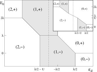
Figure 1: Ground-state phase diagram in the $E_{0}-\epsilon_{d}$ plane for $W_{0}=0$. Different regions $(\bar{N},\bar{\sigma})$ are labelled according to the ground-state dot occupation number $\bar{N}=0,1,2$ and the conformational state $\bar{\sigma}=\pm$. Dark areas correspond to $\pi$-junction behavior. The charge-degeneracy line $\epsilon_{d}=-U/2$ is indicated as dashed line. Main panel: $\lambda<U$. Inset: $\lambda>U$, where no $\pi$-junction behavior is possible for $U<E_{0}<2\lambda-U$.

By analyzing the dependence of the ground-state energy on the system parameters, one can always (even for $W_{0}\neq 0$) write the function $C(E,E^{\prime})$ in Eq. (7) as

$$C(E,E^{\prime})=\Theta(\xi_{-}-\epsilon_{d})\,C_{2}$$ (20)

$$+\,\Theta(\epsilon_{d}-\xi_{-})\,\Theta(\xi_{+}-\epsilon_{d})\,C_{1}+\Theta(\epsilon_{d}-\xi_{+})\,C_{0},$$

where $\Theta$ is the Heaviside function and the energies $\xi_{\pm}=\xi_{\pm}(U,\lambda,E_{0})$ are the boundaries enclosing the $\pi$-phase region with $\bar{N}=1$, i.e., $\xi_{+}$ ($\xi_{-}$) denotes the boundary between the $\bar{N}=0$ and $\bar{N}=1$ (the $\bar{N}=1$ and $\bar{N}=2$) regions, see Fig. 1. Explicit results for $\xi_{\pm}$ follow from Eq. (18) for $W_{0}=0$. For $E_{0}<0$ ($E_{0}>2\lambda$) and arbitrary $\bar{N}$, the ground state is realized when $\bar{\sigma}=-$ $(\bar{\sigma}=+)$, leading to $\xi_{+}=\lambda/2$ ($\xi_{+}=-\lambda/2$). In both cases, the other boundary energy follows as $\xi_{-}=\xi_{+}-U$. In the intermediate cases, with $\xi_{0}=\frac{1}{2}(\lambda-U-E_{0}),$ we find for $0<E_{0}<\lambda$,

$$\xi_{+}={\rm max}(\lambda/2-E_{0},\xi_{0}),\quad\xi_{-}={\rm min}(\lambda/2-U,\xi_{0}),$$ (21)

while for $\lambda<E_{0}<2\lambda$, we obtain

$$\xi_{+}={\rm max}(-\lambda/2,\xi_{0}),\quad\xi_{-}={\rm min}(\xi_{0},\lambda/2+2\xi_{0}).$$ (22)

These results for $\xi_{\pm}$ are summarized in Fig. 1. Remarkably, in the $E_{0}-\epsilon_{d}$ plane, the phase diagram is inversion-symmetric with respect to the point $(E_{0}=\lambda,\epsilon_{d}=-U/2)$. Furthermore, we observe that for many choices of $E_{0}$, one can switch the TLS between the $\bar{\sigma}=\pm$ states by varying $\epsilon_{d}$, see Fig. 1.

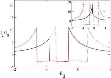
Figure 2: (Color online) Ground-state critical current $I_{c}$ as a function of $\epsilon_{d}$ for $W_{0}=0$. $I_{c}$ is given in units of $I_{0}$, see Eq. (17). In all figures, the energy scale is set by $\Delta=1$. Dashed (red), dotted (blue) and solid (black) curves represent the partial critical currents $I_{c}(\epsilon_{+})$, $I_{c}(\epsilon_{-})$, and the realized critical current $I_{c}$, respectively. Main panel: $E_{0}=0.8,\lambda=0.6,U=1$, such that $\xi_{+}>\xi_{-}$. This corresponds to the $\pi$-phase region with $\lambda<E_{0}<2\lambda$ in the main panel of Fig. 1. Inset: $E_{0}=0.6,\lambda=0.8,U=0.5$, where $\xi_{+}<\xi_{-}$ and no $\pi$-junction behavior is possible. This corresponds to $U<E_{0}<2\lambda-U$, see inset of Fig. 1.

We now notice that Eq. (20) implies the same decomposition for the critical current (7). We can therefore immediately conclude that the $\pi$-junction regime (where $\bar{N}=1)$ can exist only when $\xi_{+}>\xi_{-}$. This condition is always met away from the window $0<E_{0}<2\lambda$. However, inside that window, Eqs. (21) and (22) imply that for sufficiently strong dot-TLS coupling, $\lambda>U$, the $\pi$-phase may disappear completely. Indeed, for $U<E_{0}<2\lambda-U$, no $\pi$-phase is possible for any value of $\epsilon_{d}$ once $\lambda$ exceeds $U$. The resulting ground-state critical current is shown as a function of the dot level $\epsilon_{d}$ for two typical parameter sets in Fig. 2. The inset shows a case where the $\pi$-phase has been removed by a strong coupling of the interacting dot to the TLS. The above discussion shows that the $\pi$-junction regime is very sensitive to the presence of a strongly coupled TLS.

IV Finite TLS tunneling

Next we address the case of finite TLS tunneling, $W_{0}\neq 0$. Due to the $\sigma_{x}$ term in $H_{0}$, the critical current cannot be written anymore as a weighted sum, see Eq. (19), and no abrupt switching of the TLS happens when changing the system parameters. Nevertheless, we now show that the size and even the existence of the $\pi$-phase region still sensitively depend on the TLS coupling strength (and on the other system parameters). In particular, the $\pi$-phase can again be completely suppressed for strong $\lambda$.

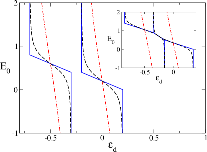
Figure 3: (Color online) Phase diagram and boundary energies $\xi_{\pm}$ enclosing the $\pi$-phase for finite $W_{0}$. Main figure: $\lambda=0.4$ and $U=0.5$, where a $\pi$-phase is present; $W_{0}=0,0.2$ and $5$, for solid (blue), dashed (black) and dash-dotted (red) curves, respectively. Inset: $\lambda=0.7$ and $U=0.5$, where the $\pi$-phase vanishes; $W_{0}=0,0.3$ and $3$, for solid (blue), dashed (black) and dash-dotted (red) curves, respectively.

For finite $W_{0}$, the ground-state critical current is obtained from Eq. (20), where the $C_{N}$ are given by Eqs. (II)–(II) and the $\pi$-phase border energies $\xi_{\pm}$ are replaced by

$$\xi_{+}=\frac{1}{2}\left(\Phi_{1}-\Phi_{0}\right),\quad\xi_{-}=\frac{1}{2}\left(\Phi_{2}-\Phi_{1}-2U\right).$$ (23)

The $\Phi_{N}$ are defined in Eq. (10). Compared to the $W_{0}=0$ case in Fig. 1, the phase diagram boundaries now have a smooth (smeared) shape due to the TLS tunneling. Nevertheless, the critical current changes sign abruptly when the system parameters are tuned across such a boundary. The energies (23) are shown in Fig. 3 for various values of $W_{0}$ in the $E_{0}-\epsilon_{d}$ plane. In between the $\xi_{+}$ and $\xi_{-}$ curves, the $\pi$-phase is realized. From the inset of Fig. 3, we indeed confirm that the $\pi$-phase can again be absent within a suitable parameter window. Just as for $W_{0}=0$, the $\pi$-phase vanishes for $\xi_{+}<\xi_{-}$, and the transition between left and right $0$-phase occurs at $\bar{\xi}=(\xi_{+}+\xi_{-})/2$. For $|E_{0}|\gg{\rm max}(\lambda,W_{0})$, we effectively recover the phase diagram for $W_{0}=0$, since the TLS predominantly occupies a fixed conformational state.

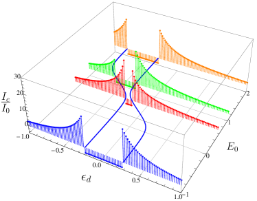
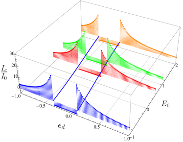
Figure 4: (Color online) Listline plots of the $W_{0}\neq 0$ ground-state critical current $I_{c}$ (in units of $I_{0}$) in the $E_{0}-\epsilon_{d}$ plane, with $\lambda=0.6$ and $U=0.5$. The boundaries $\xi_{\pm}$ enclosing the $\pi$-phase, see also Fig. 3, are indicated as solid (blue) curves. Top panel: Small tunnel amplitude, $W_{0}=0.2$. Bottom panel: Large tunnel amplitude, $W_{0}=3$.

The corresponding critical current $I_{c}$ is shown in Fig. 4 for both a small and a very large TLS tunnel matrix element $W_{0}$. In the limit of large $W_{0}\gg{\rm max}(\lambda,|E_{0}|)$, see lower panel in Fig. 4, the dot and the TLS are effectively decoupled, since $\langle\sigma_{z}\rangle\simeq 0$ and $\langle\sigma_{x}\rangle\simeq{\rm sgn}(W_{0})$. While this limit is unrealistic for molecular junctions, it may be realized in a side-coupled double-dot system.zazuprl Finally we note that, unlike for $W_{0}=0$, the perturbative result for the critical current diverges at the point where the $\pi$-phase vanishes, i.e., for $\epsilon_{d}=\bar{\xi}$. This divergence is an artefact of perturbation theory and is caused by the appearance of the factor $G_{E_{0}^{-}-E_{2}^{-}}(0)=(\epsilon_{d}-\bar{\xi})^{-1}$ in Eqs. (II) and (II).

V Conclusions

In this paper, we have presented a perturbative calculation of the critical Josephson current, $I_{c}$, through an interacting single-level molecular junction side-coupled to a two-level system (TLS). Such a TLS is a simple model for a bistable conformational degree of freedom, and has previously been introduced in the literature.zazuprl ; tls-exp1 ; fabrizio Our perturbative calculation assumes very weak coupling to attached superconducting reservoirs. The ground-state critical current can then be computed exactly for otherwise arbitrary parameters. Our main finding is that the $\pi$-phase with $I_{c}<0$ is quite sensitive to the presence of the TLS. In particular, for strong coupling $\lambda$ of the molecular level to the TLS as compared to the Coulomb energy $U$ on the level, the $\pi$-phase can disappear altogether.

Appendix A Partial critical currents

In this Appendix, we provide the partial critical current $I_{c}(\epsilon_{\sigma})$ which appears in the calculation for $W_{0}=0$, see Sec. III. In the absence of TLS tunneling, the matrix elements (16) simplify to

$$T_{N_{1}N_{2}N_{3}N_{4}}^{\sigma_{1}\sigma_{2}\sigma_{3}\sigma_{4}}=\prod_{i=1}^{4}\delta_{\tilde{\sigma}_{i},1}+\prod_{i=1}^{4}\delta_{\tilde{\sigma}_{i},-1},$$

where $\tilde{\sigma}_{i}=\sigma_{i}{\rm sgn}(N_{i}\lambda-E_{0})$. We now rename $\tilde{\sigma}\to\sigma$ to denote the conformational state (eigenstate of $\sigma_{z}$).

The partial current $I_{c}(\epsilon_{\sigma})$ corresponding to fixed conformational state $\sigma=\pm$ is then given by

$$\frac{I_{c}(\epsilon_{\sigma})}{I_{0}}=\Delta^{3}\sum_{N}\int_{\Delta}^{\infty}\frac{dEdE^{\prime}C_{N}^{\sigma}(E,E^{\prime})}{\sqrt{(E^{2}-\Delta^{2})(E^{\prime 2}-\Delta^{2})}},$$

where

$$C_{N}^{\sigma}(E,E^{\prime}) = \tilde{p}_{N}^{\sigma}c_{N}^{\sigma}(E,E^{\prime}),$$

$$\tilde{p}_{N}^{\sigma} = \frac{1}{Z_{\sigma}}e^{-\beta E_{N}^{\sigma}}\,(1+\delta_{N,1}),$$

with $Z_{\sigma}$ such that $\sum_{N}\tilde{p}_{N}^{\sigma}=1$. Moreover, the $c^{\sigma}_{N}$ are given by

$$c_{0}^{\sigma}(E,E^{\prime})=\frac{1}{(E+\epsilon_{\sigma})(E^{\prime}+\epsilon_{\sigma})}\left[\frac{1}{E+E^{\prime}}+\frac{2}{2\epsilon_{\sigma}+U}\right],$$

$$c_{1}^{\sigma}(E,E^{\prime})=-\frac{1}{E+E^{\prime}}\Big{[}\frac{1}{(E-\epsilon_{\sigma})(E+\epsilon_{\sigma}+U)}$$

$$+\,\frac{1}{(E^{\prime}-\epsilon_{\sigma})(E^{\prime}+\epsilon_{\sigma}+U)}+\frac{1/2}{(E-\epsilon_{\sigma})(E^{\prime}-\epsilon_{\sigma})}$$

$$+\,\frac{1/2}{(E+\epsilon_{\sigma}+U)(E^{\prime}+\epsilon_{\sigma}+U)}\Big{]},$$

$$c_{2}^{\sigma}(E,E^{\prime}) = \frac{1}{(E-\epsilon_{\sigma}-U)(E^{\prime}-\epsilon_{\sigma}-U)}$$

$$\times \left[\frac{1}{E+E^{\prime}}-\frac{2}{2\epsilon_{\sigma}+U}\right].$$

References

- (1) A. Nitzan and M.A. Ratner, Science 300, 1384 (2003).
- (2) N.J. Tao, Nature Nanotechnology 1, 173 (2006).
- (3) A.A. Golubov, M.Yu. Kupriyanov, and E. Il’ichev, Rev. Mod. Phys. 76, 411 (2004).
- (4) A.Yu. Kasumov, R. Deblock, M. Kociak, B. Reulet, H. Bouchiat, I.I. Khodos, Yu.B. Gorbatov, V.T. Volkov, C. Journet, and M. Burghard, Science 284, 1508 (1999).
- (5) A. Morpurgo, J. Kong, C.M. Marcus, and H. Dai, Science 286, 263 (1999).
- (6) B. Reulet, A.Yu. Kasumov, M. Kociak, R. Deblock, I.I. Khodos, Yu.B. Gorbatov, V.T. Volkov, C. Journet, and H. Bouchiat, Phys. Rev. Lett. 85, 2829 (2000).
- (7) M.R. Buitelaar, T. Nussbaumer, and C. Schönenberger, Phys. Rev. Lett. 89, 256801 (2002).
- (8) M.R. Buitelaar, W. Belzig, T. Nussbaumer, B. Babic, C. Bruder, and C. Schönenberger, Phys. Rev. Lett. 91, 057005 (2003).
- (9) Y.-J. Doh, J.A. van Dam, A.L. Roest, E.P.A.M. Bakkers, L.P. Kouwenhoven, and S. De Franceschi, Science 309, 272 (2005).
- (10) A.Yu. Kasumov, K. Tsukagoshi, M. Kawamura, T. Kobayashi, Y. Aoyagi, K. Senba, T. Kodama, H. Nishikawa, I. Ikemoto, K. Kikuchi, V.T. Volkov, Yu.A. Kasumov, R. Deblock, S. Gueron, and H. Bouchiat, Phys. Rev. B 72, 033414 (2005).
- (11) H.I. Jorgensen, K. Grove-Rasmussen, T. Novotný, K. Flensberg, and P.E. Lindelof, Phys. Rev. Lett. 96, 207003 (2006).
- (12) J. Xiang, A. Vidan, M. Tinkham, R.M. Westervelt, and C.M. Lieber, Nature Nanotech. 1, 208 (2006).
- (13) P. Jarillo-Herrero, J.A. van Dam, and L.P. Kouwenhoven, Nature (London) 439, 953 (2006).
- (14) J.A. van Dam, Yu.V. Nazarov, E.P.A.M. Bakkers, S. De Franceschi, and L.P. Kouwenhoven, Nature (London) 442, 667 (2006).
- (15) J.-P. Cleuziou, W. Wernsdorfer, V. Bouchiat, T. Ondarcuhu, and M. Monthioux, Nature Nanotechnology 1, 53 (2006).
- (16) M. Chauvin, P. vom Stein, D. Esteve, C. Urbina, J.C. Cuevas, and A. Levy Yeyati, Phys. Rev. Lett. 99, 067008 (2007).
- (17) A. Eichler, M. Weiss, S. Oberholzer, C. Schönenberger, A. Levy Yeyati, J.C. Cuevas, and A. Martin-Rodero, Phys. Rev. Lett. 99, 126602 (2007).
- (18) T. Sand-Jespersen, J. Paaske, B.M. Andersen, K. Grove-Rasmussen, H.I. Jorgensen, M. Aagesen, C.B. Sorensen, P.E. Lindelof, K. Flensberg, and J. Nygard, Phys. Rev. Lett. 99, 126603 (2007).
- (19) M.L. Della Rocca, M. Chauvin, B. Huard, H. Pothier, D. Esteve, and C. Urbina, Phys. Rev. Lett. 99, 127005 (2007).
- (20) A. Marchenkov, Z. Dai, B. Donehoo, R.H. Barnett, and U. Landman, Nature Nanotech. 2, 481 (2007).
- (21) F. Wu, R. Danneau, P. Queipo, E. Kauppinen, T. Tsuneta, and P.J. Hakonen, Phys. Rev. B 79, 073404 (2009).
- (22) A. Eichler, R. Deblock, M. Weiss, C. Karrasch, V. Meden, C. Schönenberger, and H. Bouchiat, arXiv:0810.1671.
- (23) H. Shiba and T. Soda, Prog. Theor. Phys. 41, 25 (1969).
- (24) L.I. Glazman and K.A. Matveev, JETP Lett. 49, 659 (1989)
- (25) B.I. Spivak and S.A. Kivelson, Phys. Rev. B 43, 3740 (1991).
- (26) A.V. Rozhkov and D.P. Arovas, Phys. Rev. Lett. 82, 2788 (1999).
- (27) O. Zachar, Phys. Rev. B 61, 95 (2000).
- (28) A.A. Clerk and V. Ambegaokar, Phys. Rev. B 61, 9109 (2000).
- (29) D. Matsumoto, J. Phys. Soc. Jpn. 70, 492 (2001).
- (30) E. Vecino, A. Martin-Rodero, and A.L. Yeyati, Phys. Rev. B 68, 035105 (2003).
- (31) F. Siano and R. Egger, Phys. Rev. Lett. 93, 047002 (2004).
- (32) M.S. Choi, M. Lee, K. Kang, and W. Belzig, Phys. Rev. B 70, 020502(R) (2004).
- (33) G. Sellier, T. Kopp, J. Kroha, and Y.S. Barash, Phys. Rev. B 72, 174502 (2005).
- (34) T. Novotný, A. Rossini, and K. Flensberg, Phys. Rev. B 72, 224502 (2005).
- (35) C. Karrasch, A. Oguri, and V. Meden, Phys. Rev. B 77, 024517 (2008).
- (36) T. Meng, P. Simon, and S. Florens, arXiv:0902.1111.
- (37) For finite , one also has intermediate and phases.rozhkov These phases disappear, however, in the limit considered in this work.
- (38) H.I. Jorgensen, T. Novotný, K. Grove-Rasmussen, K. Flensberg, and P.E. Lindelof, Nano Lett. 7, 2441 (2007).
- (39) A.I. Buzdin, Rev. Mod. Phys. 77, 935 (2005).
- (40) F.S. Bergeret, A.F. Volkov, and K.B. Efetov, Rev. Mod. Phys. 77, 1321 (2005).
- (41) J.X. Zhu, Z. Nussinov, A. Shnirman, and A.V. Balatsky, Phys. Rev. Lett. 92, 107001 (2004).
- (42) Z. Nussinov, A. Shnirman, D.P. Arovas, A.V. Balatsky, and J.X. Zhu, Phys. Rev. B 71, 214520 (2005).
- (43) M. Lee, T. Jonckheere, and T. Martin, Phys. Rev. Lett. 101, 146804 (2008).
- (44) J. Sköldberg, T. Löfwander, V.S. Shumeiko, and M. Fogelström, Phys. Rev. Lett. 101, 087002 (2008).
- (45) A. Zazunov, R. Egger, C. Mora, and T. Martin, Phys. Rev. B 73, 214501 (2006).
- (46) A. Zazunov, D. Feinberg, and T. Martin, Phys. Rev. Lett. 97, 196801 (2006).
- (47) A. Zazunov, A. Schulz, and R. Egger, Phys. Rev. Lett. 102, 047002 (2009).
- (48) W.H.A. Thijssen, D. Djukic, A.F. Otte, R.H. Bremmer, and J.M. van Ruitenbeek, Phys. Rev. Lett. 97, 226806 (2006).
- (49) A.V. Danilov, S.E. Kubatkin, S.G. Kafanov, K. Flensberg, and T. Bjørnholm, Nano Lett. 6, 2184 (2006).
- (50) S.Y. Quek, M. Kamenetska, M.L. Steigerwald, H.J. Choi, S.G. Louie, M.S. Hybertsen, J.B. Neaton, and L. Venkataraman, preprint arXiv:0901.1139.
- (51) A. Donarini, M. Grifoni, and K. Richter, Phys. Rev. Lett. 97, 166801 (2006).
- (52) A. Mitra and A.J. Millis, Phys. Rev. B 76, 085342 (2007).
- (53) P. Lucignano, G.E. Santoro, M. Fabrizio, and E. Tosatti, Phys. Rev. B 78, 155418 (2008).