Solution of the Crow-Kimura and Eigen models for alphabets of arbitrary size by Schwinger spin coherent states

Abstract

To represent the evolution of nucleic acid and protein sequence, we express the parallel and Eigen models for molecular evolution in terms of a functional integral representation with an $h$-letter alphabet, lifting the two-state, purine/pyrimidine assumption often made in quasi-species theory. For arbitrary $h$ and a general mutation scheme, we obtain the solution of this model in terms of a maximum principle. Euler’s theorem for homogeneous functions is used to derive this ‘thermodynamic’ formulation of evolution. The general result for the parallel model reduces to known results for the purine/pyrimidine $h=2$ alphabet and the nucleic acid $h=4$ alphabet for the Kimura 3 ST mutation scheme. Examples are presented for the $h=4$ and $h=20$ cases. We derive the maximum principle for the Eigen model for general $h$. The general result for the Eigen model reduces to a known result for $h=2$. Examples are presented for the nucleic acid $h=4$ and the amino acid $h=20$ alphabet. An error catastrophe phase transition occurs in these models, and the order of the phase transition changes from second to first order for smooth fitness functions when the alphabet size is increased beyond two letters to the generic case. As examples, we analyze the general analytic solution for sharp peak, linear, quadratic, and quartic fitness functions.

1 Introduction

There are two classical physical models of molecular evolution: the Eigen model [1, 2, 3] and the Parallel or Crow-Kimura model [4]. These models were originally formulated in the language of chemical kinetics [1], by a large system of differential equations representing the time evolution of the relative frequencies of each sequence type. Quasi-species models capture the basic microscopic processes of mutation and replication, for an infinite population of binary sequences. The most remarkable feature of these models is the existence of a phase transition, termed the ”error threshold” [1, 5], when the mutation rate is below a critical value, separating a disordered non-selective phase from an organized or ”quasi-species” phase. The quasi-species is characterized by a population of closely related mutants, rather than by identical sequences [1, 2, 3], and its emergence is related to the auto-catalytic character of the replication process [1, 5], which exponentially enriches the proportion of the fittest mutants in the population. Experimental studies provide support for quasi-species theory in the evolution of RNA viruses [6, 7].

The choice of a binary alphabet, which simplifies the mathematical and numerical analysis of the theory, represents a coarse graining of the four-letter alphabet of the nucleic acids DNA/RNA (A,C,G,T/U), by considering the two basic chemical structures of nitrogenated bases, purines (A,G) and pyrimidines (C,T/U). The choice of a four-letter alphabet represents nucleic acids. A 20-letter alphabet represents amino acids and protein structure and permits a close connection between sequence and fitness.

Most numerical and analytical studies on quasi-species models consider the binary alphabet simplification [1, 2, 3, 4]. In particular, the assumption of a binary alphabet allows for an exact mapping of the quasi-species models into a 2D Ising model [8, 9], or into a quantum spin chain [10, 11, 12, 13, 14]. An exception is [15], where a four-letter alphabet was studied by a quantum spin chain representation of the parallel model. Other approaches to the nucleic acid evolution problem have been presented in [16, 17]. In all these studies it has been shown, through the application of different methodologies, that the steady state mean fitness of the population can be expressed in terms of a maximum principle, in the limit of infinite sequence length ($N\rightarrow\infty$). The Frobenius-Perrone theorem guarantees that there is a unique steady-state population distribution. It has been shown [18] that for a general family of linear (or effectively linear) models that evolve according to a matrix $H=M+R$, with $M$ a Markov generator (typically representing mutations) and $R$ a diagonal matrix (usually representing replication or degradation) of dimension $N\rightarrow\infty$, the Frobenius-Perrone largest eigenvalue can be expressed in terms of a Raleigh-Ritz variational problem. The high dimensional variational problem can be reduced to a low-dimensional maximum principle with an error $O(1/N)$, when basic symmetries can be assumed in the evolution matrix, such as permutation invariance of the replication rate, or symmetric mutation rates, which allows for a lumping [18] of the large sequence space into sequence types or classes. This analysis was applied in [17] to obtain a variational expression for the mean fitness in the Kimura model with a four letters alphabet. We note that the Eigen model, where replication and (multiple) mutations are correlated, possesses a different algebraic structure than the general family of models studied in [18]. In the Eigen model, the evolution matrix is of the form $H=Q\times R$, with $Q$ representing the mutation matrix, and $R$ a diagonal replication matrix.

In this article, we present exact analytical solutions of the $h$-alphabet Crow-Kimura and Eigen models by means of a quantum field theory. Our method generalizes the Schwinger spin coherent field theory for the binary alphabet in [19] to an alphabet of arbitrary size $h$. This method has also been recently applied in the solution of a model that includes transfer of genetic material between sequences in quasi-species theory [20, 21], and two-parent recombination [21]. For the parallel model, we present exact analytical solutions of this field theory, in terms of a maximum principle, for the steady state mean fitness of the population and average composition, Eq. (49). We present as examples, results for the Kimura 3 ST mutation scheme [22], Eq. (54). We develop in detail the result for the symmetric mutation rate scheme, Eq. (55), for four different examples of microscopic fitness functions: sharp peak Eqs. (57) and (58), Fujiyama landscape Eqs. (60)–(63), a quadratic landscape Eqs. (65)–(69), and a quartic landscape Eqs. (71) and (72). In section 2.9, we apply our general formula to derive the mean fitness for the symmetric, general $h$ case and discuss the $h=20$ amino acid alphabet, Eq. (74). For the symmetric case, we present results for the sharp peak, Eqs. (75)–(77), and the quadratic case, Eq. (77).

For the Eigen model, we present the exact expression for arbitrary alphabet size $h$, Eq. (106). As an example, we apply the general expression to a mutation scheme analogous to the Kimura 3 ST [22], Eq. (112). We analyze in detail the solution for the symmetric mutations rate, Eq. (113), for four different examples of microscopic fitness functions: sharp peak Eqs. (114) and (115), Fujiyama landscape Eqs. (116–119), quadratic fitness landscape Eqs. (121–123), and quartic fitness landscape Eqs. (125) and (126). In section 3.8, we apply our general solution to derive the mean fitness for the symmetric, general $h$ case and discuss the $h=20$ amino acid alphabet, Eq. (127). For the symmetric case, we present results for the sharp peak, Eqs. (128)–(129), and the quadratic case.

These results bring quasi-species theory closer to the real microscopic evolutionary dynamics that occurs in the natural four-letter alphabet of nucleic acids or the 20-letter alphabet of amino acids.

2 The parallel model for an alphabet of size $h$

The parallel model [4] describes the continuous time evolution of an infinite size population of viral genetic sequences. The evolutionary dynamics is driven by point mutations and selection, with mutations occurring in parallel and independently of viral replication. Each viral genome is represented as a sequence of N letters, from an alphabet of size $h$, and therefore the total number of different viral genomes in the population is $h^{N}$. If we describe a viral genetic sequence in the alphabet of nucleic acids (DNA or RNA), the natural choice would be $h=4$, and explicitly the alphabet corresponds to (A,C,G,T or U). It is common, to simplify the theoretical analysis, to choose instead a coarse grained alphabet of size $h=2$, by ’lumping’ together purines (A, T or U) and pyrimidines (C,G). Alternatively, to describe evolution at the scale of protein sequences, the natural choice is to consider the $h=20$ amino acid alphabet. We here consider the case of general $h$.

The probability $p_{i}$ for a virus to have a genetic sequence $S_{i}$, $1\leq i\leq h^{N}$, evolves according to the following system of nonlinear differential equations

$$\frac{dp_{i}}{dt}=p_{i}(r_{i}-\sum_{j=1}^{h^{N}}r_{j}p_{j})+\sum_{j=1}^{h^{N}}\mu_{ij}p_{j}$$ (1)

Here $r_{i}$ is replication rate of sequence $S_{i}$, and $\mu_{ij}$ is the mutation rate from sequence $S_{j}$ into sequence $S_{i}$. The nonlinear term in Eq. (1) represents the average replication rate in the population, or mean fitness. This non-linear term enforces the conservation of probability, $\sum_{i}p_{i}=1$. This term can be removed through a simple exponential transformation, to obtain the linear system of differential equations

$$\frac{dq_{i}}{dt}=r_{i}q_{i}+\sum_{j=1}^{h^{N}}\mu_{ij}q_{j}$$ (2)

where $p_{i}(t)=q_{i}(t)/\sum_{j}q_{j}(t)$.

2.1 Fitness landscape

We will assume that the replication rate (fitness) of an individual in the population depends on its relative composition with respect to a wild-type sequence $S_{w}$. We define the relative composition variables, $x^{\alpha}$, to be the number of letters of type $\alpha$, divided by $N$. The number of different letters is $h$, and the set of labels $\alpha$ refers to the set of chemical possibilities, such as {purine,pyrimidine}, {A,C,G,T}, or the 20 amino acids. For an alphabet of size $h$, at each site along the sequence, there are $h-1$ independent compositions $0\leq x^{\alpha}\leq 1$, for $1\leq\alpha\leq h-1$. Alternatively, these compositions may be interpreted as normalized Hamming distances from a reference wild-type sequence. Therefore, the replication rate for a sequence $S_{i}$ in the parallel model Eq. (1) is defined by the fitness function

$$r_{i}=Nf(x^{1},x^{2},\ldots,x^{h-1})$$ (3)

where the $x^{\alpha}$ are defined within the simplex $\sum_{\alpha=1}^{h-1}x^{\alpha}\leq 1$.

2.2 Schwinger spin coherent states representation of the parallel model

We can express the parallel model in operator form, by generalizing the method presented in [19]. We define $h$ kinds of creation and annihilation operators: $\hat{a}^{\dagger}_{\alpha}(j),\hat{a}_{\alpha}(j)$, $1\leq\alpha\leq h$ and $1\leq j\leq N$. These operators satisfy the commutation relations

$$\left[\hat{a}_{\alpha}(i),\hat{a}_{\beta}^{\dagger}(j)\right]=\delta_{\alpha\beta}\delta_{ij}$$

$$\left[\hat{a}_{\alpha}(i),\hat{a}_{\beta}(j)\right]=\left[\hat{a}_{\alpha}^{\dagger}(i),\hat{a}_{\beta}^{\dagger}(j)\right]=0$$ (4)

These operators create/annihilate a sequence letter state $1\leq\alpha\leq h$, at position $1\leq j\leq N$ in the sequence. Since at each site there is a single letter, we enforce the constraint

$$\sum_{\alpha=1}^{h}\hat{a}^{\dagger}_{\alpha}(j)\hat{a}_{\alpha}(j)=1$$ (5)

for all $1\leq j\leq N$.

We define $n_{\alpha}^{i}(j)$ as the power on $\hat{a}^{\dagger}_{\alpha}(j)$ for the sequence state $S_{i}$, $1\leq i\leq h^{N}$, defined by the vectors

$$|S_{i}\rangle=\prod_{j=1}^{N}|\vec{n}^{i}_{j}\rangle$$ (6)

where $|\vec{n}^{i}_{j}\rangle=\prod_{\alpha=1}^{h}\left[\hat{a}^{\dagger}_{\alpha}(j)\right]^{n_{\alpha}^{i}(j)}|0\rangle$. The constraint in Eq. (5) ensures that the condition $\sum_{\alpha=1}^{h}n_{\alpha}^{i}(j)=1$ for all $i,j$.

We introduce the unnormalized population state vector

$$|\psi\rangle=\sum_{i=1}^{h^{N}}q(S_{i})|S_{i}\rangle$$ (7)

which evolves in time according to the equation

$$\frac{d}{dt}|\psi\rangle=-\hat{H}|\psi\rangle$$ (8)

Here, the Hamiltonian operator, to highest order in $N$, is given by

$$-\hat{H}=\hat{m}+Nf(\hat{x}^{1},\hat{x}^{2},\ldots,\hat{x}^{h-1})$$ (9)

where $\hat{m}$ represents the mutation operator, and $\hat{x}^{\alpha}$ represents the compositions in operator form.

Let us first discuss the mutation operator $\hat{m}$. In the most general case, $h(h-1)$ possible different substitutions can occur at each site in the sequence, i.e. $\beta\rightarrow\alpha$, with mutation rate $\mu_{\alpha\beta}$ that need not be symmetric.

Each individual process can be written in the operator form

$$\vec{\hat{a}}^{\dagger}(j)\tau^{\alpha\beta}\vec{\hat{a}}(j)=\hat{a}^{\dagger}_{\alpha}(j)\hat{a}_{\beta}(j)+\sum_{\gamma\neq\alpha}\hat{a}^{\dagger}_{\gamma}(j)\hat{a}_{\gamma}(j)$$ (10)

which represents the creation of letter $\alpha$ by annihilation of letter $\beta$. Here, the matrices $\tau^{\alpha\beta}$ are explicitly defined by

$$\left[\tau^{\alpha\beta}\right]_{\rho\gamma}=\delta_{\rho\alpha}\delta_{\gamma\beta}+\delta_{\rho\gamma}(1-\delta_{\rho\alpha})$$ (11)

After these definitions, the more general expression for the mutation operator is

$$\hat{m}=\sum_{j=1}^{N}\sum_{\alpha\neq\beta=1}^{h}\mu_{\alpha\beta}\left[\vec{\hat{a}}^{\dagger}(j)\tau^{\alpha\beta}\vec{\hat{a}}(j)-\vec{\hat{a}}^{\dagger}(j)\cdot\vec{\hat{a}}(j)\right]$$ (12)

Let us now consider the Schwinger spin coherent state representation of the average base composition terms,

$$\hat{x}^{\alpha}=\frac{1}{N}\sum_{j=1}^{N}\hat{a}^{\dagger}_{\alpha}(j)\hat{a}_{\alpha}(j)\equiv\frac{1}{N}\sum_{j=1}^{N}\vec{\hat{a}}^{\dagger}(j)\Theta^{\alpha}\vec{\hat{a}}(j)\,\,\,\,1\leq\alpha\leq h-1$$ (13)

where we defined the matrices

$$\left[\Theta^{\alpha}\right]_{\rho\gamma}=\delta_{\rho\alpha}\delta_{\gamma\alpha}$$ (14)

We introduce the vector notation

$$\vec{\hat{x}}=(\hat{x}^{1},\hat{x}^{2},\ldots,\hat{x}^{h-1})$$ (15)

$${\bf{\Theta}}=(\Theta^{1},\Theta^{2},\ldots,\Theta^{h-1})$$ (16)

Considering the previous expressions, the Hamiltonian operator becomes

$$-\hat{H} = Nf\left[\frac{1}{N}\sum_{j=1}^{N}\vec{\hat{a}}^{\dagger}(j)\mathbf{\Theta}\vec{\hat{a}}(j)\right]+\sum_{j=1}^{N}\sum_{\alpha\neq\beta=1}^{h}\mu_{\alpha\beta}\left[\vec{\hat{a}}^{\dagger}(j)\tau^{\alpha\beta}\vec{\hat{a}}(j)-\vec{\hat{a}}^{\dagger}(j)\cdot\vec{\hat{a}}(j)\right]$$

2.3 Functional integral representation of the parallel model

We convert the operator representation of the parallel model into a functional integral form by introducing Schwinger spin coherent states [19]. We define a coherent state by

$$|\vec{z}(j)\rangle = e^{\vec{\hat{a}}^{\dagger}(j)\cdot\vec{z}(j)-\vec{z}^{*}(j)\cdot\vec{\hat{a}}(j)}|0\rangle$$

$$= e^{-\frac{1}{2}\vec{z}^{*}(j)\cdot\vec{z}(j)}\sum_{m_{1},m_{2},\ldots,m_{h}=0}^{\infty}\prod_{\alpha=1}^{h}\frac{\left[z_{\alpha}(j)\right]^{m_{\alpha}}}{\sqrt{m_{\alpha}!}}|(m_{1},m_{2},\ldots,m_{h})_{j}\rangle$$

Coherent states satisfy the completeness relation

$$I=\int\prod_{j=1}^{N}\frac{d\vec{z}^{*}(j)d\vec{z}(j)}{\pi^{h}}|\{\vec{z}\}\rangle\langle\{\vec{z}\}|$$ (19)

The overlap between a pair of coherent states is given by

$$\langle\vec{z}^{\,{}^{\prime}}(j)|\vec{z}(j)\rangle=e^{-\frac{1}{2}\{\vec{z}^{\,{}^{\prime}*}(j)\cdot[\vec{z}^{{}^{\prime}}(j)-\vec{z}(j)]-[\vec{z}^{\,{}^{\prime}*}(j)-\vec{z}^{*}(j)]\cdot\vec{z}(j)\}}$$ (20)

To enforce the constraint Eq. (5), we introduce the projector

$$\hat{P}=\prod_{j=1}^{N}\hat{P}(j)=\prod_{j=1}^{N}\Delta[\vec{\hat{a}}^{\dagger}(j)\cdot\vec{\hat{a}}(j)-1]$$

$$=\int_{0}^{2\pi}\prod_{j=1}^{N}\frac{d\lambda_{j}}{2\pi}e^{i\lambda_{j}[\vec{\hat{a}}^{\dagger}(j)\cdot\vec{\hat{a}}(j)-1]}$$ (21)

At long times, due to the Perrone-Frobenius theorem, we find that the system evolution is dominated by the unique largest eigenvalue, $f_{m}$, of $-\hat{H}$ and its corresponding eigenvector $|\psi^{*}\rangle$, such that $e^{-\hat{H}t}|\{\vec{n}_{0}\}\rangle\sim e^{f_{m}t}|\psi^{*}\rangle$.

To evaluate this eigenvalue, we perform a Trotter factorization, for $\epsilon=t/M$, with $M\rightarrow\infty$, and introduce resolutions of the identity as defined by Eq. (19) at each time slice [19]

$$e^{-\hat{H}t}=\lim_{M\rightarrow\infty}\int\left[\prod_{k=1}^{M}\prod_{j=1}^{N}\frac{d\vec{z}^{*}_{k}(j)d\vec{z}_{k}(j)}{\pi^{h}}\right]|\{\vec{z}_{M}\}\rangle\prod_{k=1}^{M}\langle\{\vec{z}_{k}\}|e^{-\epsilon\hat{H}}|\{\vec{z}_{k-1}\}\rangle\langle\{\vec{z}_{0}\}|$$

(22)

We define the partition function

$$Z = {\rm{Tr}}\>e^{-\hat{H}t}\hat{P}$$

$$= \int_{0}^{2\pi}\left[\prod_{j=1}^{N}\frac{d\lambda_{j}}{2\pi}\right]e^{-i\lambda_{j}}\lim_{M\rightarrow\infty}\int\left[\prod_{k=1}^{M}\prod_{j=1}^{N}\frac{d\vec{z}^{*}_{k}(j)d\vec{z}_{k}(j)}{\pi^{h}}\right]e^{-S[\vec{z}^{*},\vec{z}]}$$

Here, we defined

$$e^{-S[\vec{z}^{*},\vec{z}]}=\prod_{k=1}^{M}\langle\{\vec{z}_{k}\}|e^{-\epsilon\hat{H}}|\{\vec{z}_{k-1}\}\rangle$$ (24)

with the boundary condition $\vec{z}_{0}(j)=e^{i\lambda_{j}}\vec{z}_{M}(j)$ [19]. An explicit expression for the matrix element in the coherent states representation is

$$\langle\{\vec{z}_{k}\}|e^{-\epsilon\hat{H}}|\{\vec{z}_{k-1}\}\rangle = \exp\bigg{(}-\frac{1}{2}\sum_{j=1}^{N}[\vec{z}_{k}^{*}(j)\cdot\vec{z}_{k}(j)-2\vec{z}_{k}^{*}(j)\cdot\vec{z}_{k-1}(j)+\vec{z}_{k-1}^{*}(j)\cdot\vec{z}_{k-1}(j)]$$

$$- \epsilon N\sum_{\alpha\neq\beta=1}^{h}\mu_{\alpha\beta}+\epsilon Nf\left[\frac{1}{N}\sum_{j=1}^{N}\vec{z}_{k}^{*}(j)\mathbf{\Theta}\vec{z}_{k-1}(j)\right]$$

$$+ \epsilon\sum_{j=1}^{N}\vec{z}^{*}_{k}(j)\sum_{\alpha\neq\beta=1}^{h}\mu_{\alpha\beta}\tau^{\alpha\beta}\vec{z}_{k-1}(j)\bigg{)}$$

Let us now introduce an ($h$-1)-component vector field $\vec{x}_{k}=(x_{k}^{1},x_{k}^{2},\ldots,x_{k}^{h-1})$, with

$$x_{k}^{\alpha}=\frac{1}{N}\sum_{j=1}^{N}\vec{z}_{k}^{*}(j)\Theta^{\alpha}\vec{z}_{k-1}(j)$$ (26)

We make this definition by introducing an integral representation of the corresponding delta function

$$1 = \int\mathcal{D}[\vec{x}]\prod_{k=1}^{M}\delta^{(h-1)}\left[\vec{x}_{k}-\frac{1}{N}\sum_{j=1}^{N}\vec{z}_{k}^{*}(j)\mathbf{\Theta}\vec{z}_{k-1}(j)\right]$$

$$= \int\left[\prod_{k=1}^{M}\prod_{\alpha=1}^{h-1}\frac{d\bar{x}_{k}^{\alpha}dx_{k}^{\alpha}}{2\pi}\right]e^{i\sum_{k=1}^{M}\vec{\bar{x}}_{k}\cdot\vec{x}_{k}-\frac{i}{N}\sum_{k=1}^{M}\sum_{j=1}^{N}\vec{z}^{*}_{k}(j)\vec{\bar{x}}_{k}\cdot\mathbf{\Theta}\vec{z}_{k-1}(j)}$$

$$= \int\left[\prod_{k=1}^{M}\prod_{\alpha=1}^{h-1}\frac{i\epsilon Nd\bar{x}_{k}^{\alpha}dx_{k}^{\alpha}}{2\pi}\right]e^{-\epsilon N\sum_{k=1}^{M}\vec{\bar{x}}_{k}\cdot\vec{x}_{k}+\epsilon\sum_{k=1}^{M}\sum_{j=1}^{N}\vec{z}^{*}_{k}(j)\vec{\bar{x}}_{k}\cdot\mathbf{\Theta}\vec{z}_{k-1}(j)}$$

Inserting this into the functional integral Eq. (LABEL:eq36), we have [19]

$$Z = \lim_{M\rightarrow\infty}\int\mathcal{D}[\vec{\bar{x}}]\mathcal{D}[\vec{x}]e^{\epsilon N\sum_{k=1}^{M}[f(\vec{x}_{k})-\vec{\bar{x}}_{k}\cdot\vec{x}_{k}-\sum_{\alpha\neq\beta=1}^{h}\mu_{\alpha\beta}]}$$ (28)

$$\times\int\mathcal{D}[\vec{z}^{*}]\mathcal{D}[\vec{z}]\mathcal{D}[\lambda]\prod_{j=1}^{N}e^{-i\lambda_{j}}e^{\epsilon\sum_{l,k=1}^{M}\vec{z}^{*}_{k}(j)S_{kl}(j)\vec{z}_{l}(j)}\bigg{|}_{\{\vec{z}_{0}\}=\{e^{i\lambda_{j}}\vec{z}_{M}\}}$$

The matrix $S(j)$ has the structure

$$S(j)=\left(\begin{array}[]{ccccc}I&0&0&\ldots&-e^{-i\lambda_{j}}A_{1}(j)\\ -A_{2}(j)&I&0&\ldots&0\\ 0&-A_{3}(j)&I&\ldots&0\\ &&&\ddots&\\ 0&&\ldots&-A_{M}(j)&I\end{array}\right)$$ (34)

where $A_{k}(j)=I+\epsilon[\sum_{\alpha\neq\beta=1}^{h}\mu_{\alpha\beta}\tau^{\alpha\beta}+\vec{\bar{x}}_{k}\cdot\mathbf{\Theta}]$. After performing the Gaussian integration over the coherent state fields, we obtain

$$Z = \lim_{M\rightarrow\infty}\int\mathcal{D}[\vec{\bar{x}}]\mathcal{D}[\vec{x}]e^{\epsilon N\sum_{k=1}^{M}[f(\vec{x}_{k})-\vec{\bar{x}}_{k}\cdot\vec{x}_{k}-\sum_{\alpha\neq\beta=1}^{h}\mu_{\alpha\beta}]}$$ (35)

$$\times\int\mathcal{D}[\lambda]\prod_{j=1}^{N}e^{-i\lambda_{j}}\left[\det S(j)\right]^{-1}$$

Here,

$$\det S(j) = \det\left[I-e^{i\lambda_{j}}\prod_{k=1}^{M}A_{k}(j)\right]$$ (36)

$$= \det\left[I-e^{i\lambda_{j}}\hat{T}e^{\epsilon\sum_{k=1}^{M}[\sum_{\alpha\neq\beta=1}^{h}\mu_{\alpha\beta}\tau^{\alpha\beta}+\vec{\bar{x}}_{k}\cdot\mathbf{\Theta}]}\right]$$

$$= e^{{\rm{Tr}}\ln\left[I-e^{i\lambda_{j}}\hat{T}e^{\epsilon\sum_{k=1}^{M}[\sum_{\alpha\neq\beta=1}^{h}\mu_{\alpha\beta}\tau^{\alpha\beta}+\vec{\bar{x}}_{k}\cdot\mathbf{\Theta}]}\right]}$$

where the operator $\hat{T}$ indicates time ordering. Substituting this result in the partition function, we obtain

$$Z = \lim_{M\rightarrow\infty}\int\mathcal{D}[\vec{\bar{x}}]\mathcal{D}[\vec{x}]e^{\epsilon N\sum_{k=1}^{M}[f(\vec{x}_{k})-\vec{\bar{x}}_{k}\cdot\vec{x}_{k}-\sum_{\alpha\neq\beta=1}^{h}\mu_{\alpha\beta}]}$$ (37)

$$\times\int\mathcal{D}[\lambda]\prod_{j=1}^{N}e^{-i\lambda_{j}}e^{-{\rm{Tr}}\ln\left[I-e^{i\lambda_{j}}\hat{T}e^{\epsilon\sum_{k=1}^{M}[\sum_{\alpha\neq\beta=1}^{h}\mu_{\alpha\beta}\tau^{\alpha\beta}+\vec{\bar{x}}_{k}\cdot\mathbf{\Theta}]}\right]}$$

$$= \lim_{M\rightarrow\infty}\int\mathcal{D}[\vec{\bar{x}}]\mathcal{D}[\vec{x}]e^{\epsilon N\sum_{k=1}^{M}[f(\vec{x}_{k})-\vec{\bar{x}}_{k}\cdot\vec{x}_{k}-\sum_{\alpha\neq\beta=1}^{h}\mu_{\alpha\beta}]}\prod_{j=1}^{N}Q$$

with

$$Q = \lim_{M\rightarrow\infty}{\rm{Tr}}\>\hat{T}\prod_{k=1}^{M}\left[I+\epsilon(\sum_{\alpha\neq\beta=1}^{h}\mu_{\alpha\beta}\tau^{\alpha\beta}+\vec{\bar{x}}_{k}\cdot\mathbf{\Theta})\right]$$ (38)

$$= \lim_{M\rightarrow\infty}{\rm{Tr}}\>\hat{T}e^{\epsilon\sum_{k=1}^{M}[\sum_{\alpha\neq\beta=1}^{h}\mu_{\alpha\beta}\tau^{\alpha\beta}+\vec{\bar{x}}_{k}\cdot\mathbf{\Theta}]}$$

$$= {\rm{Tr}}\>\hat{T}e^{\int_{0}^{t}dt^{\prime}[\sum_{\alpha\neq\beta=1}^{h}\mu_{\alpha\beta}\tau^{\alpha\beta}+\vec{\bar{x}}(t^{\prime})\cdot\mathbf{\Theta}]}$$

After taking the limit $M\rightarrow\infty$, Eq. (37) becomes

$$Z=\int\mathcal{D}[\vec{\bar{x}}]\mathcal{D}[\vec{x}]e^{-S[\vec{\bar{x}},\vec{x}]}$$ (39)

where the effective action is given by

$$S[\vec{\bar{x}},\vec{x}] = -N\int_{0}^{t}dt^{\prime}[f(\vec{x}(t^{\prime}))-\vec{\bar{x}}(t^{\prime})\cdot\vec{x}(t^{\prime})-\sum_{\alpha\neq\beta=1}^{h}\mu_{\alpha\beta}]-N\ln Q$$

Here, we have defined

$$Q={\rm{Tr}}\>\hat{T}e^{\int_{0}^{t}dt^{\prime}[\sum_{\alpha\neq\beta=1}^{h}\mu_{\alpha\beta}\tau^{\alpha\beta}+\sum_{\alpha=1}^{h-1}\bar{x}^{\alpha}(t^{\prime})\Theta^{\alpha}]}$$ (41)

2.4 The large N limit of the parallel model is a saddle point

Considering that the sequence length N is very large, $N\rightarrow\infty$, we can evaluate the functional integral Eq. (39) for the partition function by looking for a saddle point. With the action defined in Eq. (41), we have

$$\frac{\delta S}{\delta x^{\alpha}}\bigg{|}_{\vec{x}_{c},\vec{\bar{x}}_{c}} = -N\left(\frac{\partial f[\vec{x}]}{\partial x^{\alpha}}\bigg{|}_{c}-\bar{x}_{c}^{\alpha}\right)=0$$

$$\frac{\delta S}{\delta\bar{x}^{\alpha}}\bigg{|}_{\vec{x}_{c},\vec{\bar{x}}_{c}} = -N\left(-x_{c}^{\alpha}+\frac{1}{Q}\frac{\delta Q}{\delta\bar{x}^{\alpha}}\bigg{|}_{\vec{x}_{c},\vec{\bar{x}}_{c}}\right)=0$$ (42)

We denote the value of the action at the saddle point by $S_{c}$. We have therefore the system of equations

$$\bar{x}_{c}^{\alpha} = \frac{\partial f[\vec{x}]}{\partial x^{\alpha}}\bigg{|}_{c}$$ (43)

$$x_{c}^{\alpha}=\langle\Theta^{\alpha}\rangle, 1\leq\alpha\leq h-1$$ (44)

where we defined

$$\langle(\cdot)\rangle=\frac{{\rm{Tr}}(\cdot)e^{t[\sum_{\alpha\neq\beta=1}^{h}\mu_{\alpha\beta}\tau^{\alpha\beta}+\sum_{\alpha=1}^{h-1}\bar{x}_{c}^{\alpha}\Theta^{\alpha}]}}{{\rm{Tr}}e^{t[\sum_{\alpha\neq\beta=1}^{h}\mu_{\alpha\beta}\tau^{\alpha\beta}+\sum_{\alpha=1}^{h-1}\bar{x}_{c}^{\alpha}\Theta^{\alpha}]}}$$ (45)

After this saddle-point analysis, we obtain a general expression for the mean fitness $f_{m}$ of the population, for an arbitrary microscopic fitness function $f(\vec{x})$,

$$f_{m}=\lim_{N,t\rightarrow\infty}\frac{-S_{c}}{Nt}=\max_{\{\vec{x}_{c},\vec{\bar{x}}_{c}\}}\left[f(\vec{x}_{c})-\vec{\bar{x}}_{c}\cdot\vec{x}_{c}-\sum_{\alpha\neq\beta=1}^{h}\mu_{\alpha\beta}+\lambda_{\max}\right]$$ (46)

with $\lambda_{\max}$ defined as

$$\lambda_{\rm{max}}=\lim_{t\rightarrow\infty}\frac{\ln Q}{t}$$ (47)

and corresponding to the largest eigenvalue of the matrix

$${\mathbf{M}}(\vec{\bar{x}}_{c},\{\mu_{\alpha\beta}\})=\sum_{\alpha\neq\beta=1}^{h}\mu_{\alpha\beta}\tau^{\alpha\beta}+\sum_{\alpha=1}^{h-1}\bar{x}_{c}^{\alpha}\Theta^{\alpha}$$ (48)

As shown in detail in Appendix 1, the compositions $\bar{x}^{\alpha}_{c}$ can be eliminated to reduce Eq. (46) to the final expression

$$f_{m}^{(h)} = \max_{\{x^{1}_{c},x^{2}_{c},\ldots,x^{h-1}_{c}\}}\bigg{\{}f(x^{1}_{c},x^{2}_{c},\ldots,x^{h-1}_{c})+\sum_{\alpha\neq\beta=1}^{h-1}\mu_{\alpha\beta}\left[\sqrt{x^{\alpha}_{c}x^{\beta}_{c}}-x^{\alpha}_{c}\right]$$ (49)

$$+\sum_{\alpha=1}^{h-1}\mu_{\alpha h}\left[\sqrt{x^{\alpha}_{c}\left(1-\sum_{\gamma=1}^{h-1}x^{\gamma}_{c}\right)}-x^{\alpha}_{c}\right]$$

$$+\sum_{\beta=1}^{h-1}\mu_{h\beta}\left[\sqrt{\left(1-\sum_{\gamma=1}^{h-1}x^{\gamma}_{c}\right)x^{\beta}_{c}}+\sum_{\gamma=1}^{h-1}x^{\gamma}_{c}-1\right]\bigg{\}}$$

Here, the compositions $0\leq x_{c}^{\alpha}\leq 1$ are defined within the simplex $\sum_{\alpha=1}^{h-1}x_{c}^{\alpha}\leq 1$.

2.5 The purine/pyrimidine alphabet $h$=2

Most analytical and numerical studies of quasi-species models have been formulated in the past [19, 20, 12, 14] by using a coarse-grained alphabet of nucleotides, where the nucleotide bases are lumped into purines and pyrimidines, and hence $h=2$. The maximum principle for this binary alphabet can be derived from the general expression (49), by assuming a symmetric mutation rate $\mu_{12}=\mu_{21}=\mu$, and by noticing that a single composition $x_{c}^{1}\equiv x_{c}$ (or normalized Hamming distance) is required in this case,

$$f_{m}^{(2)}=\max_{\{0\leq x_{c}\leq 1\}}\bigg{\{}f(x_{c})+\mu[2\sqrt{x_{c}(1-x_{c})}-1]\bigg{\}}$$ (50)

It is customary to use in this case a magnetization coordinate [19, 20, 12, 14] defined as $\xi_{c}=1-2x_{c}$, and hence Eq. (50) becomes

$$f_{m}^{(2)}=\max_{\{-1\leq\xi_{c}\leq 1\}}\bigg{\{}f(\xi_{c})+\mu\sqrt{1-\xi_{c}^{2}}-\mu\bigg{\}}$$ (51)

Eq. (51) is a well known result, which has been obtained in the past with different methods [14, 12], including a version of the Schwinger boson method employed in the present work [19]. It is a special case of Eq. (49).

2.6 The nucleic acid alphabet $h=4$

In the nucleic acids RNA or DNA, the alphabet is constituted by the monomers of these polymeric chains, which are $h=4$

Figure 1: The generalized mutation scheme

different nucleotides A, C, G, T/U. The general mutation scheme displayed in Fig. 1 is represented by setting $h=4$ in our general solution Eq. (49), with 3 independent compositions (or normalized Hamming distances) $x^{1}_{c}$, $x^{2}_{c}$, $x^{3}_{c}$

$$f_{m} = \max_{\{x^{1}_{c},x^{2}_{c},x^{3}_{c}\}}\bigg{\{}f(x^{1}_{c},x^{2}_{c},x^{3}_{c})+\sum_{\alpha\neq\beta=1}^{3}\mu_{\alpha\beta}\left[\sqrt{x^{\alpha}_{c}x^{\beta}_{c}}-x^{\alpha}_{c}\right]$$ (52)

$$+\sum_{\alpha=1}^{3}\mu_{\alpha 4}\left[\sqrt{x^{\alpha}_{c}\left(1-\sum_{\gamma=1}^{3}x^{\gamma}_{c}\right)}-x^{\alpha}_{c}\right]$$

$$+\sum_{\beta=1}^{3}\mu_{4\beta}\left[\sqrt{\left(1-\sum_{\gamma=1}^{3}x^{\gamma}_{c}\right)x^{\beta}_{c}}+\sum_{\gamma=1}^{3}x^{\gamma}_{c}-1\right]\bigg{\}}$$

Here, the compositions $x_{c}^{\alpha}$ are defined within the simplex $x^{1}_{c}+x^{2}_{c}+x^{3}_{c}\leq 1$.

An interesting reduction of this general model is provided by the Kimura 3 ST mutation scheme [22, 15, 16, 17], Fig. 2.

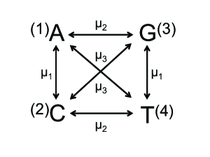
Figure 2: The Kimura 3 ST mutation scheme

The Kimura 3 ST mutation scheme considers mutations in three independent directions, with rates $\mu_{1},\mu_{2},\mu_{3}$

$$X\begin{array}[]{l}\nearrow\raise 5.0pt\hbox{$\mu_{1}$}\\ \rightarrow\mu_{2}\\ \searrow\lower 5.0pt\hbox{$\mu_{3}$}\end{array}$$

Accordingly, three components of the Hamming distance between a pair of sequences $S_{i}$ and $S_{j}$ are defined as follows

$$d_{1}(S_{i},S_{j})=\#_{A\leftrightarrow C}(S_{i},S_{j})+\#_{G\leftrightarrow T}(S_{i},S_{j})$$

$$d_{2}(S_{i},S_{j})=\#_{A\leftrightarrow G}(S_{i},S_{j})+\#_{C\leftrightarrow T}(S_{i},S_{j})$$ (53)

$$d_{3}(S_{i},S_{j})=\#_{A\leftrightarrow T}(S_{i},S_{j})+\#_{C\leftrightarrow G}(S_{i},S_{j})$$

Here, $\#_{X\leftrightarrow Y}(S_{i},S_{j})$ is the number of sites at which X and Y are exchanged between sequences $S_{i}$ and $S_{j}$. The total Hamming distance between sequences $S_{i}$ and $S_{j}$ is given by

$$d(S_{i},S_{j})=d_{1}(S_{i},S_{j})+d_{2}(S_{i},S_{j})+d_{3}(S_{i},S_{j})$$ (54)

The mutation rate is therefore modeled by the function

$$\mu_{ij}=\left\{\begin{array}[]{ll}\mu_{\alpha},&d_{\alpha}(S_{i},S_{j})=d(S_{i},S_{j})=1\\ -N\sum_{\alpha=1}^{3}\mu_{\alpha},&S_{i}=S_{j}\\ 0,&d(S_{i},S_{j})>1\end{array}\right.$$ (58)

To be consistent with existing notation in the quasispecies literature, we define 3 independent variables, which are simply transformations of the composition variables, and which are called ‘surplus’ variables in the literature

$$u_{1}(S_{i})=1-\frac{2}{N}[d_{1}(S_{i},S_{w})+d_{3}(S_{i},S_{w})]$$

$$u_{2}(S_{i})=1-\frac{2}{N}[d_{2}(S_{i},S_{w})+d_{3}(S_{i},S_{w})]$$ (59)

$$u_{3}(S_{i})=1-\frac{2}{N}[d_{1}(S_{i},S_{w})+d_{2}(S_{i},S_{w})]$$

Notice that according to this definition, the maximum value of $u=(u_{1}+u_{2}+u_{3})/3=1$ is reached when $d_{1}=d_{2}=d_{3}=0$, that is the sequence $S_{i}$ being identical to the wild type $S_{w}$. The minimum value for the average base composition is obtained when one of the Hamming distance components, say $d_{i}=N$, while the others are null $d_{j\neq i}=0$. Then, $d=d_{i}=N$ and $u=-1/3$.

The Kimura 3ST mutation scheme result is obtained from the general Eq. (52) if the following symmetries are assumed for the mutation rates

$$\mu_{12} = \mu_{21}=\mu_{34}=\mu_{43}\equiv\mu_{1}$$

$$\mu_{13} = \mu_{31}=\mu_{24}=\mu_{42}\equiv\mu_{2}$$

$$\mu_{14} = \mu_{41}=\mu_{23}=\mu_{32}\equiv\mu_{3}$$ (60)

We follow the quasispecies literature convention and define the 3 independent ‘ancestral distribution’ coordinates $\xi^{\alpha}_{c}$ (the subscript c denoting the saddle-point limit), after Eq. (2.6)

$$\xi_{c}^{1} = 1-2(x^{1}_{c}+x^{3}_{c})$$

$$\xi_{c}^{2} = 1-2(x^{2}_{c}+x^{3}_{c})$$

$$\xi_{c}^{3} = 1-2(x^{1}_{c}+x^{2}_{c})$$

The ancestral distribution variable $\xi$ is defined as the steady state analog of the ‘surplus,’ but for the time-reversed evolution process [23].

After some algebra, we obtain

$$f_{m} = \max_{\{\xi_{c}^{1},\xi_{c}^{2},\xi_{c}^{3}\}}\bigg{\{}f(\xi_{c}^{1},\xi_{c}^{2},\xi_{c}^{3})-(\mu_{1}+\mu_{2}+\mu_{3})$$ (62)

$$+\frac{\mu_{1}}{2}[\sqrt{(1+\xi_{c}^{1}+\xi_{c}^{2}+\xi_{c}^{3})(1-\xi_{c}^{1}-\xi_{c}^{2}+\xi_{c}^{3})}$$

$$+\sqrt{(1+\xi_{c}^{1}-\xi_{c}^{2}-\xi_{c}^{3})(1-\xi_{c}^{1}+\xi_{c}^{2}-\xi_{c}^{3})}]$$

$$+\frac{\mu_{2}}{2}[\sqrt{(1+\xi_{c}^{1}+\xi_{c}^{2}+\xi_{c}^{3})(1+\xi_{c}^{1}-\xi_{c}^{2}-\xi_{c}^{3})}$$

$$+\sqrt{(1-\xi_{c}^{1}+\xi_{c}^{2}-\xi_{c}^{3})(1-\xi_{c}^{1}-\xi_{c}^{2}+\xi_{c}^{3})}]$$

$$+\frac{\mu_{3}}{2}[\sqrt{(1+\xi_{c}^{1}+\xi_{c}^{2}+\xi_{c}^{3})(1-\xi_{c}^{1}+\xi_{c}^{2}-\xi_{c}^{3})}$$

$$+\sqrt{(1+\xi_{c}^{1}-\xi_{c}^{2}-\xi_{c}^{3})(1-\xi_{c}^{1}-\xi_{c}^{2}+\xi_{c}^{3})}]\bigg{\}}$$

From this general expression, the average composition ‘surplus’ $\vec{u}=(u_{1},u_{2},u_{3})$ is obtained by applying the self-consistent condition $f(\vec{u})=f_{m}$. This result is equivalent to that derived by [17].

2.7 Analytic results for the symmetric mutational scheme

For a symmetric mutational scheme, $\mu_{1}=\mu_{2}=\mu_{3}\equiv\mu$, we specialize the general Eq. (62) by setting $\xi_{c}^{1}=\xi_{c}^{2}=\xi_{c}^{3}\equiv\xi_{c}$, and $u_{i}=u$, and thus obtaining an expression for the mean fitness

$$f_{m}=\max_{-\frac{1}{3}\leq\xi_{c}\leq 1}\left\{f(\xi_{c})-\frac{3}{2}\mu(1+\xi_{c})+\frac{3}{2}\mu\sqrt{(1-\xi_{c})(1+3\xi_{c})}\right\}$$

(63)

This result is equivalent to that derived by [17]. We remark that Eq. (63) represents an exact analytical expression for the mean fitness of the population, for any arbitrary microscopic fitness $f(u)$, with the assumption of symmetric mutation rates $\mu_{1}=\mu_{2}=\mu_{3}=\mu$. From this exact expression, the average composition $u$ is obtained by applying the self-consistency condition $f_{m}=f(u)$. In the following sections, we apply Eq. (63) to analyze in detail some examples of microscopic fitness functions: The sharp peak landscape, a Fujiyama landscape, a quadratic fitness landscape, and a quartic fitness landscape. We note that the $h=2$ case contains a symmetry in the mutation terms about $\xi=0$. In the general $h>2$, this symmetry will be lost. As we will see, loss of this symmetry leads to a change in the order of the error catastrophe phase transition.

2.7.1 The sharp peak landscape

We shall first consider the sharp peak landscape, which is described by the function

$$f(u)=A\delta_{u,1}$$ (64)

That is, only sequences identical to the wild-type replicate with a rate $A>0$. From Eq. (63), we notice that this implies: $\xi_{c}=1$, if $A>3\mu$, or $\xi_{c}=0$ otherwise. Therefore, we obtain for the mean replication rate

$$f_{m}=\left\{\begin{array}[]{cc}A-3\mu,&A>3\mu\\ 0,&A<3\mu\end{array}\right.$$ (67)

The fraction of the population at the wild-type $p_{w}$ is obtained from the self-consistent condition $f_{m}=p_{w}A$,

$$p_{w}=\left\{\begin{array}[]{cc}1-\frac{3\mu}{A},&A>3\mu\\ 0,&A<3\mu\end{array}\right.$$ (70)

There exists an error threshold in this case, which is given by the critical value $A_{crit}=3\mu$, as shown in Eqs. (67), (70) and displayed in Fig. 3. The phase transition is first order as a function of $A/\mu$.

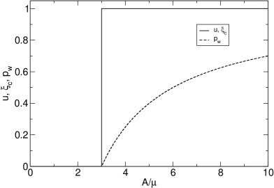
Figure 3: Average composition $u$, magnetization $\xi_{c}$ and fraction of the population at the wild-type sequence $p_{w}$, as a function of the parameter $A/\mu$, for the sharp peak fitness.

One may compare this result with the error threshold observed in the binary alphabet case, which is [19] $A_{crit}=\mu$. This result is intuitive, because in the 4 letters alphabet, there exist 3 mutation channels to escape from the wild type instead of just one as in the binary alphabet, and therefore a stronger selection pressure is required to retain the wild-type features.

2.7.2 The Fujiyama fitness landscape

The Fujiyama landscape is obtained as a linear function of the composition

$$f[\vec{u}]=\alpha_{1}u_{1}+\alpha_{2}u_{2}+\alpha_{3}u_{3}$$ (71)

We will present analytical results for the symmetric case $\alpha_{i}\equiv\alpha$, $\mu_{i}\equiv\mu$. Thus, $\xi_{c}^{1}=\xi_{c}^{2}=\xi_{c}^{3}=\xi_{c}$. Substituting in Eq. (63), we have

$$f_{m}=\max_{-\frac{1}{3}\leq\xi_{c}\leq 1}\left\{3\alpha\xi_{c}-\frac{3}{2}\mu(1+\xi_{c})+\frac{3}{2}\mu\sqrt{(1-\xi_{c})(1+3\xi_{c})}\right\}$$ (72)

We look for a maximum

$$\frac{\partial f_{m}}{\partial\xi_{c}}=3\alpha-\frac{3}{2}\mu+\frac{3}{2}\mu\frac{2-6\xi_{c}}{2\sqrt{1+2\xi_{c}-3\xi_{c}^{2}}}=0$$ (73)

From this equation, we obtain

$$\xi_{c}=\frac{1}{3}\left(1+\frac{2\alpha-\mu}{\sqrt{\alpha^{2}-\alpha\mu+\mu^{2}}}\right)$$ (74)

To obtain the average base composition $u$, we apply the self-consistent condition $f_{m}=f(u)=3\alpha u$, to obtain

$$u=\frac{1}{3}\left(1-2\frac{\mu}{\alpha}+\frac{2}{\alpha}\sqrt{\alpha^{2}-\mu\alpha+\mu^{2}}\right)$$ (75)

Clearly, no phase transition is observed in this fitness landscape, as $0<u<1$ for $0<\alpha<\infty$. This result is in agreement with the analysis presented in [15], were a quantum spin chain formulation was employed.

2.7.3 Quadratic fitness landscape

The quadratic fitness landscape is given by the general quadratic form

$$f(\vec{u})=\sum_{i=1}^{3}(\frac{\beta_{i}}{2}u_{i}^{2}+\alpha_{i}u_{i})$$ (76)

We will present the analytical solution for the symmetric case $\alpha_{i}\equiv\alpha$, $\beta_{i}\equiv\beta$, with the symmetric mutation scheme $\mu_{i}\equiv\mu$. Under these conditions, we have $\xi_{c}^{1}=\xi_{c}^{2}=\xi_{c}^{3}\equiv\xi_{c}$, and from Eq. (63) we have for the mean fitness

$$f_{m}=\max_{-\frac{1}{3}\leq\xi_{c}\leq 1}\left\{\frac{3}{2}\beta\xi_{c}^{2}+3\alpha\xi_{c}-\frac{3}{2}\mu(1+\xi_{c})+\frac{3}{2}\mu\sqrt{(1-\xi_{c})(1+3\xi_{c})}\right\}$$ (77)

The maximum is obtained from the equation

$$\frac{\partial f_{m}}{\partial\xi_{c}}=3\beta\xi_{c}+3\alpha-\frac{3}{2}\mu+\frac{3}{2}\mu\frac{2-6\xi_{c}}{2\sqrt{1+2\xi_{c}-3\xi_{c}^{2}}}=0$$ (78)

From Eq. (78), we obtain

$$\beta\xi_{c}+\alpha-\frac{\mu}{2}=\frac{\mu}{2}\frac{3\xi_{c}-1}{\sqrt{1+2\xi_{c}-3\xi_{c}^{2}}}$$ (79)

As shown in Appendix 2, this equation can be cast in the form of a quartic equation, whose roots are the values of $\xi_{c}$. The average composition $u$ is finally obtained through the self-consistency equation

$$f_{m}=f(u)=\frac{3}{2}\beta u^{2}+3\alpha u$$ (80)

We find that the error threshold transition towards a selective phase for $\alpha=0$ is defined by $\xi_{c}>0$, $u>0$, at $\beta>3/2\mu$. The value of $u$ is continuous at the transition, as it is straightforward to check from Eq. (78) $f_{m}(\xi_{c}=0)=f_{m}(\xi_{c}=2/3,\beta=3\mu/2)=0$, which implies after Eq. (80) (for $\alpha=0$) that $u=0$ when approaching the critical point $\beta=3\mu/2$ from both sides. However, $\xi_{c}$ jumps from 0 [for $\beta\rightarrow(3\mu/2)^{-}$] to 2/3 [for $\beta\rightarrow(3\mu/2)^{+}$] (Appendix 2). To analyze the order of the transition, we expand Eq. (77) as a quadratic polynomial in $\xi_{c}$ in a neighborhood of the critical point $\beta\simeq 3\mu/2$,

$$f_{m}(\xi_{c})=\left\{\begin{array}[]{cc}\frac{3}{2}(\beta-3\mu/2)\xi_{c}^{2}&,\beta<3\mu/2\\ \frac{2}{3}\beta-\mu+(2\beta-3\mu)(\xi_{c}-\frac{2}{3})+(\frac{3}{2}\beta-3\mu)(\xi_{c}-\frac{2}{3})^{2}&,\beta>3\mu/2\end{array}\right.$$ (83)

(84)

we find that the first derivative $df_{m}/d\beta[\beta\rightarrow(3\mu/2)^{-}]=0$, while $df_{m}/d\beta[\beta\rightarrow(3\mu/2)^{+}]=2/3$, and thus it has a discontinuous jump from $0$ to $2/3$. Therefore, the phase transition is first order as a function of $\beta/\mu$. We notice that the order of the phase transition, for a similar quadratic fitness landscape, is found to be of second order for a binary alphabet [19].

When $0\leq\alpha/\beta\leq\frac{1}{3}\left(\sqrt{\frac{4}{3}}-1\right)$, as shown in Appendix 2, we find a finite jump in the magnetization from $\xi_{c,+}$ to $\xi_{c,-}$, with $\xi_{c,\pm}=1/3(1\pm\sqrt{1-18\alpha/\beta-27(\alpha/\beta)^{2}})$. This result is in agreement with [15], where an alternative method of quantum spin chains was applied for the derivation. A complete analysis of the different possible cases other than this, is presented in Appendix 2.

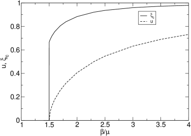
Figure 4: Average composition $u$ and magnetization $\xi_{c}$ as a function of the parameter $\beta/\mu$, for the quadratic fitness when $\alpha=0$.

2.8 Quartic fitness landscape

As a final example, we consider a quartic fitness landscape

$$f(\vec{u})=\sum_{i=1}^{3}\frac{\beta_{i}}{4}u_{i}^{4}$$ (85)

As in the previous cases, we consider the symmetric mutation rates $\mu_{i}\equiv\mu$, $\beta_{i}\equiv\beta$, and hence $\xi_{c,i}\equiv\xi_{c}$. Considering this fitness function in the general equation (63), we have that the mean fitness is given by the analytical expression

$$f_{m}=\max_{\{-\frac{1}{3}\leq\xi_{c}\leq 1\}}\bigg{\{}\frac{3}{4}\beta\xi_{c}^{4}-\frac{3}{2}\mu(1+\xi_{c})+\frac{3}{2}\mu\sqrt{(1-\xi_{c})(1+3\xi_{c})}\bigg{\}}$$ (86)

The average composition $u$ is obtained by applying the self-consistent condition

$$f(u)=\frac{3}{4}\beta u^{4}=f_{m}$$ (87)

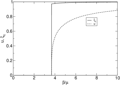
Figure 5: Average composition $u$ and magnetization $\xi_{c}$ as a function of the parameter $\beta/\mu$, for the quartic fitness landscape.

In Fig. 5, we present the values of $u$ and $\xi_{c}$, as obtained from Eqs. (86), (87), as a function of the parameter $\beta/\mu$. A discontinuous jump in the bulk magnetization from $\xi_{c}=0$ to $\xi_{c}=0.971618$ is observed at $\beta/\mu=3.67653$. By expanding Eq. (86) near the critical point, after similar procedure as in the quadratic fitness case, we find a discontinuous jump in the derivative $df_{m}/d\beta$, from $0$ to $0.66841101$. Therefore, the phase transition is first order in $\beta/\mu$. The average composition $u$, however, experiences a fast but smooth transition. This behavior is much alike the one observed in the sharp peak fitness landscape, Eq. (67) and Fig. (3), except for the fact that the average composition $u$ is continuous at the transition. Indeed, from a purely mathematical perspective, a fitness function following a power law $f_{n}(u)=ku^{n}$, for $0<u<1$, will satisfy the limit

$$\lim_{n\rightarrow\infty}f_{n}(u)=k\delta_{u,1}$$ (88)

which is precisely the sharp peak landscape, Eq. (64).

2.9 Symmetric case, general h, with application to the amino acid alphabet $h=20$

An alternative language to describe molecular evolution is in terms of mutation and selection acting over the translated protein sequence, which is drawn from an $h=20$ amino acid alphabet. For the parallel model, the time evolution of an infinite population of protein sequences is described by the system of differential equations (2), with $h=20$. Thus, we are lead to consider the $h=20$ case. We first consider the symmetric case with general $h$.

For an alphabet of arbitrary size $h$, a symmetrical mutation scheme $\mu_{\alpha\beta}=\mu$, and a symmetrical fitness function that leads to $x^{\alpha}_{c}=x_{c}$, we define a magnetization coordinate $\xi_{c}=1-hx_{c}$, and Eq. (49) reduces to

$$f_{m} = \max_{\{-1/(h-1)\leq\xi_{c}\leq 1\}}\bigg{\{}f(\xi_{c})+(h-1)\mu[\frac{2}{h}\sqrt{(1-\xi_{c})(1+(h-1)\xi_{c})}$$ (89)

$$+\frac{h-2}{h}(1-\xi_{c})-1]\bigg{\}}$$

As an example of application of Eq. (89), we consider the sharp peak fitness landscape $f(\xi_{c})=A\delta_{\xi_{c},1}$. Then, from Eq. (89) we obtain the mean fitness

$$f_{m}=\left\{\begin{array}[]{cc}A-(h-1)\mu,&A>(h-1)\mu\\ 0,&A\leq(h-1)\mu\end{array}\right.$$ (92)

We obtain the fraction of sequences in the wild type, $p_{w}$, by applying the self-consistency condition $f_{m}=Ap_{w}$, which yields

$$p_{w}=\left\{\begin{array}[]{cc}1-\frac{(h-1)\mu}{A},&A>(h-1)\mu\\ 0,&A\leq(h-1)\mu\end{array}\right.$$ (95)

This result is intuitive, since there exists $h-1$ independent mutation channels for the sequence to escape from the wild type. Moreover, for a general alphabet of size $h$, a first order phase transition occurs at the critical point $A_{\rm{crit}}^{h}=(h-1)\mu$.

As a second example, we consider the quadratic fitness landscape for an alphabet of size $h$, $f(\xi_{c})=(h-1)\beta\xi_{c}^{2}/2$. For the quadratic fitness function we can work out the order of the phase transition for general $h$. We consider $f(\xi)=(h-1)\beta\xi^{2}/2$. There is a phase transition at $\beta_{crit}=2\mu(h-1)/h$. The magnetization jumps from $\xi_{c}=0$ at $\beta\rightarrow\beta_{crit}^{-}$ to $\xi_{c}=(h-2)/(h-1)$ at $\beta\rightarrow\beta_{crit}^{+}$. The first derivative at the critical point is:

$$\frac{df_{m}}{d\beta}=\left\{\begin{array}[]{cc}0,&\beta<2\mu(h-1)/h\\ (h-2)^{2}/[2(h-1)],&\beta>2\mu(h-1)/h\end{array}\right.$$ (98)

Thus, the jump in the first derivative is $(h-2)^{2}/[2(h-1)]$. Thus, the transition is second order for $h=2$ and first order for $h>2$.

3 The $h$-states Eigen model

The Eigen model conceptually differs from the parallel or Kimura model because it is assumed that mutations arise as a consequence of errors in the replication process. For an alphabet of size $h$, the system of equations which describes the time evolution of the probabilities $p_{i}$, with $1\leq i\leq h^{N}$, is

$$\frac{dp_{i}}{dt}=\sum_{j=1}^{N}[B_{ij}r_{j}-\delta_{ij}D_{j}]p_{j}-p_{i}\left[\sum_{j=1}^{N}(r_{j}-D_{j})p_{j}\right]$$ (99)

Here, $r_{i}$ is the replication rate of sequence $S_{i}$, and the components of the matrix

$$B_{ij}=(1-q)^{N-d_{ij}}\left(\frac{q}{h-1}\right)^{d_{ij}}$$ (100)

represent the transition rates from sequence $S_{j}$ into $S_{i}$, where $1-q$ is the probability to copy a nucleotide without error, and $q$ is the probability per site for a base substitution during the replication process.

We consider a generalized version of this, by considering that the base substitution probabilities are not necessarily identical nor symmetric. That is, for a base substitution $\beta\rightarrow\alpha$, we consider a probability $q_{\alpha\beta}\neq q_{\beta\alpha}$. Correspondingly, we define $h-1$ independent base compositions $0\leq x^{\alpha}\leq 1$, which can also be interpreted as normalized Hamming distances with respect to the $h$-th reference species, $x^{\alpha}=d^{\alpha}/N$. For this generalized mutation scheme, the transition rate matrix components are defined by

$$B_{ij}=(1-q)^{N(1-\sum_{\alpha=1}^{h-1}x^{\alpha})}\prod_{\alpha\neq\beta=1}^{h}\left(q_{\alpha\beta}\right)^{Nx^{\alpha}}$$ (101)

Here, $q=\sum_{\alpha\neq\beta=1}^{h}q_{\alpha\beta}$, and the $x^{\alpha}$ are as in Sec. 2.1.

3.1 The $h$-states Eigen model in operator form

By similar arguments as in the parallel model, we formulate a Hamiltonian operator for the Eigen model

$$-\hat{H} = \prod_{j=1}^{N}\left[(1-q)\vec{\hat{a}}^{\dagger}(j)\cdot\vec{\hat{a}}(j)+\sum_{\alpha\neq\beta=1}^{h}q_{\alpha\beta}\vec{\hat{a}}^{\dagger}(j)\tau^{\alpha\beta}\vec{\hat{a}}(j)\right]$$ (102)

$$\times Nf\left[\frac{1}{N}\sum_{l=1}^{N}\vec{\hat{a}}^{\dagger}(l)\mathbf{\Theta}\vec{\hat{a}}(l)\right]-Nd\left[\frac{1}{N}\sum_{l=1}^{N}\vec{\hat{a}}^{\dagger}(l)\mathbf{\Theta}\vec{\hat{a}}(l)\right]$$

Here, the matrices $\tau^{\alpha\beta}$ are defined as in the parallel model by Eq. (11) and in the matrix array ${\mathbf{\Theta}}=(\Theta^{1},\Theta^{2},\ldots,\Theta^{h-1})$, the matrices $\Theta^{\alpha}$ are defined as in Eq. (14). Let us define the coefficients $\mu_{\alpha\beta}=Nq_{\alpha\beta}$. The degradation function is given by $D_{i}=Nd(x^{1},x^{2},\ldots,x^{h-1})$. Then, we have for $q\ll 1$

$$-N\ln(1-q)\simeq Nq = N\sum_{\alpha\neq\beta=1}^{h}q_{\alpha\beta}=\sum_{\alpha\neq\beta=1}^{h}\mu_{\alpha\beta}$$ (103)

The Hamiltonian operator Eq. (102) is expressed, to $\mathcal{O}(1/N)$, by

$$-\hat{H} = Ne^{-\sum_{\alpha\neq\beta=1}^{h}\mu_{\alpha\beta}}e^{\sum_{j=1}^{N}\left[\sum_{\alpha\neq\beta=1}^{h}\frac{\mu_{\alpha\beta}}{N}\vec{\hat{a}}^{\dagger}(j)\tau^{\alpha\beta}\vec{\hat{a}}(j)\right]}$$ (104)

$$\times f\left[\frac{1}{N}\sum_{l=1}^{N}\vec{\hat{a}}^{\dagger}(l)\mathbf{\Theta}\vec{\hat{a}}(l)\right]-Nd\left[\frac{1}{N}\sum_{l=1}^{N}\vec{\hat{a}}^{\dagger}(l)\mathbf{\Theta}\vec{\hat{a}}(l)\right]$$

To study the equilibrium properties of the system, as in the case of the parallel model, we calculate the partition function by performing a Trotter factorization

$$Z = {\rm{Tr}}\>e^{-\hat{H}t}\hat{P}$$

$$= \int_{0}^{2\pi}\left[\prod_{j=1}^{N}\frac{d\lambda_{j}}{2\pi}\right]e^{-i\lambda_{j}}\lim_{M\rightarrow\infty}\int\left[\prod_{k=1}^{M}\prod_{j=1}^{N}\frac{d^{h}\vec{z}_{k}^{*}(j)d^{h}\vec{z}_{k}(j)}{\pi^{h}}\right]e^{-S[\vec{z}^{*},\vec{z}]}$$

Here,

$$e^{-S[\vec{z}^{*},\vec{z}]}=\prod_{k=1}^{M}\langle\{\vec{z}_{k}\}|e^{-\epsilon\hat{H}}|\{\vec{z}_{k-1}\}\rangle$$ (106)

where the matrix elements in the coherent states basis are given by the expression

$$\langle\{\vec{z}_{k}\}|e^{-\epsilon\hat{H}}|\{\vec{z}_{k-1}\}\rangle = e^{-\frac{1}{2}\sum_{j=1}^{N}(\vec{z}^{*}_{k}(j)\cdot\vec{z}_{k}(j)-2\vec{z}_{k}^{*}(j)\cdot\vec{z}_{k-1}(j)+\vec{z}_{k-1}^{*}(j)\cdot\vec{z}_{k-1}(j))}$$

$$\times\exp\bigg{(}\epsilon Ne^{-\sum_{\alpha\neq\beta=1}^{h}\mu_{\alpha\beta}}e^{\frac{1}{N}\sum_{j=1}^{N}\vec{z}_{k}^{*}(j)\left(\sum_{\alpha\neq\beta=1}^{h}\mu_{\alpha\beta}\tau^{\alpha\beta}\right)\vec{z}_{k-1}(j)}$$

$$\times f\left[\frac{1}{N}\sum_{j=1}^{N}\vec{z}^{*}_{k}(j)\mathbf{\Theta}\vec{z}_{k-1}(j)\right]-\epsilon Nd\left[\frac{1}{N}\sum_{j=1}^{N}\vec{z}^{*}_{k}(j)\mathbf{\Theta}\vec{z}_{k-1}(j)\right]\bigg{)}$$

Let us introduce the $(h-1)$-component vector field $\vec{x}_{k}=(x_{k}^{1},x_{k}^{2},\ldots,x_{k}^{h-1})$, and an integral representation of the corresponding delta function

$$1 = \int\mathcal{D}[\vec{x}]\prod_{k=1}^{M}\delta^{(h-1)}\left[\vec{x}_{k}-\frac{1}{N}\sum_{j=1}^{N}\vec{z}_{k}^{*}(j)\mathbf{\Theta}\vec{z}_{k-1}(j)\right]$$

$$= \int\left[\prod_{k=1}^{M}\prod_{\alpha=1}^{h-1}\frac{i\epsilon Nd\bar{x}_{k}^{\alpha}dx_{k}^{\alpha}}{2\pi}\right]e^{-\epsilon N\sum_{k=1}^{M}\vec{\bar{x}}_{k}\cdot\vec{x}_{k}+\epsilon\sum_{k=1}^{M}\sum_{j=1}^{N}\vec{z}^{*}_{k}(j)\vec{\bar{x}}_{k}\cdot\mathbf{\Theta}\vec{z}_{k-1}(j)}$$

Similarly, let us introduce a second set of fields $\eta^{\alpha\beta}$,

$$1 = \int\mathcal{D}[\eta^{\alpha\beta}]\prod_{k=1}^{M}\delta\left[\eta_{k}^{\alpha\beta}-\frac{1}{N}\sum_{j=1}^{N}\vec{z}_{k}^{*}(j)\tau^{\alpha\beta}\vec{z}_{k-1}(j)\right]$$

$$= \int\left[\prod_{k=1}^{M}\frac{i\epsilon Nd\bar{\eta}_{k}^{\alpha\beta}d\eta_{k}^{\alpha\beta}}{2\pi}\right]$$

$$\times e^{-\epsilon N\sum_{k=1}^{M}\bar{\eta}_{k}^{\alpha\beta}\eta_{k}^{\alpha\beta}+\epsilon\sum_{k=1}^{M}\bar{\eta}_{k}^{\alpha\beta}\sum_{j=1}^{N}\vec{z}_{k}^{*}(j)\tau^{\alpha\beta}\vec{z}_{k-1}(j)}$$

Inserting both constraints Eq. (LABEL:eq90) and Eq. (LABEL:eq91) in the expression for the trace Eq. (LABEL:eq87), we obtain

$$Z = \lim_{M\rightarrow\infty}\int\mathcal{D}[\vec{x}]\mathcal{D}[\vec{\bar{x}}]\prod_{\alpha\neq\beta}\mathcal{D}[\eta^{\alpha\beta}]\mathcal{D}[\bar{\eta}^{\alpha\beta}]$$ (110)

$$\times e^{\epsilon N\sum_{k=1}^{M}(-\vec{\bar{x}}_{k}\cdot\vec{x}_{k}-\sum_{\alpha\neq\beta=1}^{h}\bar{\eta}_{k}^{\alpha\beta}\eta_{k}^{\alpha\beta}+e^{\sum_{\alpha\neq\beta=1}^{h}\mu_{\alpha\beta}(\eta^{\alpha\beta}-1)}f[\vec{x}_{k}]-d[\vec{x}_{k}])}$$

$$\times\int\mathcal{D}[\vec{z}^{*}]\mathcal{D}[\vec{z}]\mathcal{D}[\lambda]\prod_{j=1}^{N}e^{-i\lambda_{j}}e^{\epsilon\sum_{k,l=1}^{M}\vec{z}_{k}^{*}(j)S_{kl}\vec{z}_{l}(j)}\bigg{|}_{\{\vec{z}_{0}\}=\{e^{i\lambda_{j}}\vec{z}_{M}\}}$$

After performing the Gaussian integral over the fields $\vec{z}^{*},\vec{z}$, we obtain

$$Z = \lim_{M\rightarrow\infty}\int\mathcal{D}[\vec{x}]\mathcal{D}[\vec{\bar{x}}]\prod_{\alpha\neq\beta}\mathcal{D}[\eta^{\alpha\beta}]\mathcal{D}[\bar{\eta}^{\alpha\beta}]$$ (111)

$$\times e^{\epsilon N\sum_{k=1}^{M}(-\vec{\bar{x}}_{k}\cdot\vec{x}_{k}-\sum_{\alpha\neq\beta=1}^{h}\bar{\eta}_{k}^{\alpha\beta}\eta_{k}^{\alpha\beta}+e^{-\sum_{\alpha\neq\beta=1}^{h}\mu_{\alpha\beta}(1-\eta^{\alpha\beta}_{k})}f[\vec{x}_{k}]-d[\vec{x}_{k}])}$$

$$\times\mathcal{D}[\lambda]\prod_{j=1}^{N}e^{-i\lambda_{j}}[\det S(j)]^{-1}$$

The matrix $S(j)$ has the structure

$$S(j)=\left(\begin{array}[]{ccccc}I&0&0&\ldots&-e^{-i\lambda_{j}}A_{1}(j)\\ -A_{2}(j)&I&0&\ldots&0\\ 0&-A_{3}(j)&I&\ldots&0\\ &&&\ddots&\\ 0&&\ldots&-A_{M}(j)&I\end{array}\right)$$ (117)

where $A_{k}(j)=I+\epsilon[\sum_{\alpha\neq\beta=1}^{h}\mu_{\alpha\beta}\bar{\eta}^{\alpha\beta}_{k}+\vec{\bar{x}}_{k}\cdot\mathbf{\Theta}]$. We obtain

$$\det S(j) = \det\left[I-e^{i\lambda_{j}}\prod_{k=1}^{M}A_{k}(j)\right]$$ (118)

$$= \det\left[I-e^{i\lambda_{j}}\hat{T}e^{\epsilon\sum_{k=1}^{M}[\sum_{\alpha\neq\beta=1}^{h}\bar{\eta}^{\alpha\beta}_{k}\tau^{\alpha\beta}+\vec{\bar{x}}_{k}\cdot\mathbf{\Theta}]}\right]$$

$$= e^{{\rm{Tr}}\ln\left[I-e^{i\lambda_{j}}\hat{T}e^{\epsilon\sum_{k=1}^{M}[\sum_{\alpha\neq\beta=1}^{h}\bar{\eta}^{\alpha\beta}_{k}\tau^{\alpha\beta}+\vec{\bar{x}}_{k}\cdot\mathbf{\Theta}]}\right]}$$

Substituting this last expression into the functional integral Eq. (111), and then performing the integrals over the $\lambda$ fields, we obtain

$$Z = \lim_{M\rightarrow\infty}\int\mathcal{D}[\vec{\bar{x}}]\mathcal{D}[\vec{x}]\prod_{\alpha\neq\beta=1}^{h}\mathcal{D}[\bar{\eta}^{\alpha\beta}]\mathcal{D}[\eta^{\alpha\beta}]$$

$$\times e^{\epsilon N\sum_{k=1}^{M}(-\vec{\bar{x}}_{k}\cdot\vec{x}_{k}-\sum_{\alpha\neq\beta=1}^{h}\bar{\eta}_{k}^{\alpha\beta}\eta_{k}^{\alpha\beta}+e^{\sum_{\alpha\neq\beta=1}^{h}\mu_{\alpha\beta}(\eta^{\alpha\beta}-1)}f[\vec{x}_{k}]-d[\vec{x}_{k}])}\prod_{j=1}^{N}Q$$

Here,

$$Q = \lim_{M\rightarrow\infty}{\rm{Tr}}\,\hat{T}\prod_{k=1}^{M}[I+\epsilon(\sum_{\alpha\neq\beta=1}^{h}\bar{\eta}_{k}^{\alpha\beta}\tau^{\alpha\beta}+\vec{\bar{x}}_{k}\cdot\mathbf{\Theta})]$$ (120)

$$= \lim_{M\rightarrow\infty}{\rm{Tr}}\,\hat{T}e^{\epsilon\sum_{k=1}^{M}[\sum_{\alpha\neq\beta=1}^{h}\bar{\eta}_{k}^{\alpha\beta}\tau^{\alpha\beta}+\vec{\bar{x}}_{k}\cdot\mathbf{\Theta}]}$$

$$= {\rm{Tr}}\,\hat{T}e^{\int_{0}^{t}dt^{\prime}[\sum_{\alpha\neq\beta=1}^{h}\bar{\eta}^{\alpha\beta}(t^{\prime})\tau^{\alpha\beta}+\vec{\bar{x}}(t^{\prime})\cdot\mathbf{\Theta}]}$$

After taking the limit $M\rightarrow\infty$, we obtain

$$Z=\int\mathcal{D}[\vec{\bar{x}}]\mathcal{D}[\vec{x}]\prod_{\alpha\neq\beta}\mathcal{D}[\bar{\eta}^{\alpha\beta}]\mathcal{D}[\eta^{\alpha\beta}]e^{-S[\vec{\bar{x}},\vec{x},\{\bar{\eta}^{\alpha\beta}\},\{\eta^{\alpha\beta}\}]}$$ (121)

Here,

$$S[\vec{\bar{x}},\vec{x},\{\bar{\eta}^{\alpha\beta}\},\{\eta^{\alpha\beta}\}] = -N\int_{0}^{t}dt^{\prime}\{-\vec{\bar{x}}(t^{\prime})\cdot\vec{x}(t^{\prime})-\sum_{\alpha\neq\beta=1}^{h}\bar{\eta}^{\alpha\beta}(t^{\prime})\eta^{\alpha\beta}(t^{\prime})$$

$$+e^{\sum_{\alpha\neq\beta=1}^{h}\mu_{\alpha\beta}(\eta^{\alpha\beta}(t^{\prime})-1)}f[\vec{x}(t^{\prime})]-d[\vec{x}(t^{\prime})]\}-N\ln Q$$

where

$$Q={\rm{Tr}}\>\hat{T}e^{\int_{0}^{t}dt^{\prime}[\sum_{\alpha\neq\beta=1}^{h}\bar{\eta}^{\alpha\beta}(t^{\prime})\tau^{\alpha\beta}+\sum_{\alpha=1}^{h-1}\bar{x}^{\alpha}(t^{\prime})\Theta^{\alpha}]}$$ (123)

With this last simplification, the effective action becomes

$$S[\vec{\bar{x}},\vec{x},\{\bar{\eta}^{\alpha\beta}\},\{\eta^{\alpha\beta}\}] = -N\int_{0}^{t}dt^{\prime}(-\vec{\bar{x}}(t^{\prime})\cdot\vec{x}(t^{\prime})-\sum_{\alpha\neq\beta=1}^{h}\bar{\eta}^{\alpha\beta}(t^{\prime})\eta^{\alpha\beta}(t^{\prime})$$

$$+e^{\sum_{\alpha\neq\beta=1}^{h}\mu_{\alpha\beta}(\eta^{\alpha\beta}-1)}f[\vec{x}(t^{\prime})]-d[\vec{x}(t^{\prime})])-N\ln Q$$

3.2 The large N limit of the $h$-state Eigen model is a saddle point

By assuming that the sequence length N is very large, $N\rightarrow\infty$, we can evaluate the functional integral Eq. (121) by a saddle point method. Considering the action defined in Eq. (LABEL:eq102), we have

$$\frac{\delta S}{\delta x^{\alpha}}\bigg{|}_{\vec{\bar{x}}_{c},\vec{x}_{c},\{\bar{\eta}_{c}^{\alpha\beta}\},\{\eta_{c}^{\alpha\beta}\}} = N\left(\bar{x}_{c}^{\alpha}-e^{\sum_{\gamma\neq\rho=1}^{h}\mu_{\gamma\rho}(\eta^{\gamma\rho}_{c}-1)}\frac{\partial f[\vec{x}]}{\partial x^{\alpha}}\bigg{|}_{c}+\frac{\partial d[\vec{x}_{c}]}{\partial x^{\alpha}}\bigg{|}_{c}\right)=0$$

$$\frac{\delta S}{\delta\eta^{\alpha\beta}}\bigg{|}_{\vec{\bar{x}}_{c},\vec{x}_{c},\{\bar{\eta}_{c}^{\alpha\beta}\},\{{\eta}_{c}^{\alpha\beta}\}} = N\left(\bar{\eta}_{c}^{\alpha\beta}-\mu_{\alpha\beta}e^{\sum_{\gamma\neq\rho=1}^{h}\mu_{\gamma\rho}(\eta^{\gamma\rho}_{c}-1)}f[\vec{x}_{c}]\right)=0$$

$$\frac{\delta S}{\delta\bar{x}^{\alpha}}\bigg{|}_{\vec{\bar{x}}_{c},\vec{x}_{c},\{\bar{\eta}^{\alpha\beta}_{c}\},\{\eta_{c}^{\alpha\beta}\}} = N\left(x_{c}^{\alpha}-\frac{1}{Q}\frac{\delta Q}{\delta\bar{x}^{\alpha}}\bigg{|}_{c}\right)=0$$

$$\frac{\delta S}{\delta\bar{\eta}^{\alpha\beta}}\bigg{|}_{\vec{\bar{x}}_{c},\vec{x}_{c},\{\bar{\eta}_{c}^{\alpha\beta}\},\{\eta_{c}^{\alpha\beta}\}} = N\left(\eta_{c}^{\alpha\beta}-\frac{1}{Q}\frac{\delta Q}{\delta\bar{\eta}^{\alpha\beta}}\bigg{|}_{c}\right)=0$$ (125)

We have therefore the system of equations

$$\bar{x}_{c}^{\alpha}=e^{\sum_{\gamma\neq\rho=1}^{h}\mu_{\gamma\rho}(\eta_{c}^{\gamma\rho}-1)}\frac{\partial f[\vec{x}]}{\partial x^{\alpha}}\bigg{|}_{c}-\frac{\partial d[\vec{x}_{c}]}{\partial x^{\alpha}}\bigg{|}_{c}$$ (126)

$$\bar{\eta}_{c}^{\alpha\beta}=\mu_{\alpha\beta}e^{\sum_{\gamma\neq\rho=1}^{h}\mu_{\gamma\rho}(\eta_{c}^{\gamma\rho}-1)}f[\vec{x}_{c}]$$ (127)

$$x_{c}^{\alpha}=\langle\Theta^{\alpha}\rangle$$ (128)

$$\eta_{c}^{\alpha\beta}=\langle\tau^{\alpha\beta}\rangle$$ (129)

where we defined

$$\langle(\cdot)\rangle=\frac{{\rm{Tr}}\>(\cdot)e^{t[\sum_{\alpha\neq\beta=1}^{h}\bar{\eta}^{\alpha\beta}_{c}\tau^{\alpha\beta}+\sum_{\alpha=1}^{h-1}\bar{x}^{\alpha}_{c}\Theta^{\alpha}]}}{{\rm{Tr}}\>e^{t[\sum_{\alpha\neq\beta=1}^{h}\bar{\eta}_{c}^{\alpha\beta}\tau^{\alpha\beta}+\sum_{\alpha=1}^{h-1}\bar{x}^{\alpha}_{c}\Theta^{\alpha}]}}$$

(130)

After the saddle-point analysis, we obtain an exact analytical expression for the mean fitness $f_{m}$ of the population, in the limit of very large sequences $N\rightarrow\infty$, for an arbitrary microscopic fitness function $f(\vec{x})$ and degradation rate $d(\vec{x})$

$$f_{m}=\lim_{N,t\rightarrow\infty}\frac{-S_{c}}{Nt} = \max_{\{\vec{x}_{c}\vec{\bar{x}}_{c},\{\eta_{c}^{\alpha\beta}\},\{\bar{\eta}_{c}^{\alpha\beta}\}\}}[e^{\sum_{\alpha\neq\beta=1}^{h}\mu_{\alpha\beta}(\eta^{\alpha\beta}_{c}-1)}f(\vec{x}_{c})-d(\vec{x}_{c})$$

$$-\vec{\bar{x}}_{c}\cdot\vec{x}_{c}-\sum_{\alpha\neq\beta=1}^{h}\eta^{\alpha\beta}_{c}\bar{\eta}^{\alpha\beta}_{c}+\lambda_{\max}]$$

As shown in Appendix 3, the $\eta^{\alpha\beta}$ can be eliminated in terms of the compositions, to obtain the final expression

$$f_{m} = \max_{\{x^{1}_{c},x^{2}_{c},\ldots,x^{h-1}_{c}\}}\bigg{\{}f(x^{1}_{c},x^{2}_{c},\ldots,x^{h-1}_{c})e^{\sum_{\alpha\neq\beta=1}^{h-1}\mu_{\alpha\beta}[\sqrt{x^{\alpha}_{c}x^{\beta}_{c}}-x^{\alpha}_{c}]}$$

$$\times e^{\sum_{\alpha=1}^{h-1}\mu_{\alpha h}[\sqrt{x^{\alpha}_{c}\left(1-\sum_{\gamma=1}^{h-1}x^{\gamma}_{c}\right)}-x^{\alpha}_{c}]}$$

$$\times e^{\sum_{\beta=1}^{h-1}\mu_{h\beta}[\sqrt{\left(1-\sum_{\gamma=1}^{h-1}x_{c}^{\gamma}\right)x^{\beta}_{c}}+\sum_{\gamma=1}^{h-1}x^{\gamma}_{c}-1]}-d(x^{1}_{c},x^{2}_{c},\ldots,x^{h-1}_{c})\bigg{\}}$$

Here, the compositions $0\leq x_{c}^{\alpha}\leq 1$ are defined within the simplex $\sum_{\alpha=1}^{h-1}x_{c}^{\alpha}\leq 1$. We note that the mutation terms in Eq.  (LABEL:eqGeEig20_1) are the exponential of the mutation terms in Eq. (49), which is a result of the mutation terms in the Eigen Hamiltonian, Eq. (104), being the exponential of those in the parallel Hamiltonian, Eq. (LABEL:eq30).

3.3 The purine/pyrimidine alphabet $h$=2

As an application of our general solution Eq. (LABEL:eqGeEig20_1), we first consider the purine/pyrimidine alphabet with $h=2$. The maximum principle for this binary alphabet can be derived from Eq. (LABEL:eqGeEig20_1) by assuming a symmetric mutation rate $\mu_{12}=\mu_{21}\equiv\mu$, and by noticing that a single composition (or normalized Hamming distance) $x_{c}^{1}\equiv x_{c}$ is required in this case,

$$f_{m}^{(2)}=\max_{0\leq x_{c}\leq 1}\left\{e^{\mu[2\sqrt{x_{c}(1-x_{c})}-1]}-d(x_{c})\right\}$$ (133)

It is customary to use in this case a magnetization coordinate, defined as $\xi_{c}=1-2x_{c}$, and hence Eq. (133) becomes

$$f_{m}^{(2)}=\max_{\{-1\leq\xi_{c}\leq 1\}}\left\{e^{\mu[\sqrt{1-\xi_{c}^{2}}-1]}f(\xi_{c})-d(\xi_{c})\right\}$$ (134)

Eq. (134) is a well known result [19, 14], and a special case of our general result Eq. (LABEL:eqGeEig20_1).

3.4 The nucleic acid alphabet $h=4$

For a general, non-symmetric mutation scheme as in Fig. 1, by considering $h=4$ in our general result Eq. (LABEL:eqGeEig20_1) we obtain

$$f_{m} = \max_{\{x^{1}_{c},x^{2}_{c},x^{3}_{c}\}}\bigg{\{}f(x^{1}_{c},x^{2}_{c},x^{3}_{c})e^{\sum_{\alpha\neq\beta=1}^{3}\mu_{\alpha\beta}[\sqrt{x^{\alpha}_{c}x^{\beta}_{c}}-x^{\alpha}_{c}]}e^{\sum_{\alpha=1}^{3}\mu_{\alpha 4}[\sqrt{x^{\alpha}_{c}\left(1-\sum_{\gamma=1}^{3}x^{\gamma}_{c}\right)}-x^{\alpha}_{c}]}$$ (135)

$$\times e^{\sum_{\beta=1}^{3}\mu_{4\beta}[\sqrt{\left(1-\sum_{\gamma=1}^{3}x_{c}^{\gamma}\right)x^{\beta}_{c}}+\sum_{\gamma=1}^{3}x^{\gamma}_{c}-1]}-d(x^{1}_{c},x^{2}_{c},x^{3}_{c})\bigg{\}}$$

Here, the compositions $x^{\alpha}_{c}$ are defined within the simplex $x^{1}_{c}+x^{2}_{c}+x^{3}_{c}\leq 1$.

An interesting reduction of this general model is provided by the Kimura 3ST mutation scheme, introduced in section 2.6, and represented in Fig. 2. We obtain the solution for the Kimura 3ST mutation scheme by assuming the following symmetries in the mutation coefficients

$$\mu_{12} = \mu_{21}=\mu_{34}=\mu_{43}\equiv\mu_{1}$$

$$\mu_{13} = \mu_{31}=\mu_{24}=\mu_{42}\equiv\mu_{2}$$

$$\mu_{14} = \mu_{41}=\mu_{23}=\mu_{32}\equiv\mu_{3}$$ (136)

along with the magnetization coordinates $\xi_{c}^{\alpha}$ defined in agreement with Eq. (136),

$$\xi_{c}^{1} = 1-2(x^{1}_{c}+x^{3}_{c})$$

$$\xi_{c}^{2} = 1-2(x^{2}_{c}+x^{3}_{c})$$

$$\xi_{c}^{3} = 1-2(x^{1}_{c}+x^{2}_{c})$$ (137)

With these assumptions, after some algebra, Eq. (LABEL:eqGeEig20_1) reduces to the expression for the Kimura 3ST scheme,

$$f_{m} = \max_{\{\xi^{1}_{c},\xi^{2}_{c},\xi^{3}_{c}\}}\bigg{\{}e^{\mu_{1}(\frac{1}{2}\sqrt{(1+\xi_{c}^{1}+\xi_{c}^{2}+\xi_{c}^{3})(1-\xi_{c}^{1}-\xi_{c}^{2}+\xi_{c}^{3})}+\frac{1}{2}\sqrt{(1+\xi_{c}^{1}-\xi_{c}^{2}-\xi_{c}^{3})(1-\xi_{c}^{1}+\xi_{c}^{2}-\xi_{c}^{3})}-1)}$$ (138)

$$\times e^{\mu_{2}(\frac{1}{2}\sqrt{(1+\xi_{c}^{1}+\xi_{c}^{2}+\xi_{c}^{3})(1+\xi_{c}^{1}-\xi_{c}^{2}-\xi_{c}^{3})})+\frac{1}{2}\sqrt{(1-\xi_{c}^{1}+\xi_{c}^{2}-\xi_{c}^{3})(1-\xi_{c}^{1}-\xi_{c}^{2}+\xi_{c}^{3})}-1)}$$

$$\times e^{\mu_{3}(\frac{1}{2}\sqrt{(1+\xi_{c}^{1}+\xi_{c}^{2}+\xi_{c}^{3})(1-\xi_{c}^{1}+\xi_{c}^{2}-\xi_{c}^{3})}+\frac{1}{2}\sqrt{(1+\xi_{c}^{1}-\xi_{c}^{2}-\xi_{c}^{3})(1-\xi_{c}^{1}-\xi_{c}^{2}+\xi_{c}^{3})}-1)}$$

$$\times f(\xi_{c}^{1},\xi_{c}^{2},\xi^{3}_{c})-d(\xi^{1}_{c},\xi^{2}_{c},\xi^{3}_{c})\bigg{\}}$$

3.5 Analytical results for the symmetric mutation scheme

If the mutation rates are identical $\mu_{1}=\mu_{2}=\mu_{3}=\mu$, then we have the symmetric case $\xi_{c}^{1}=\xi_{c}^{2}=\xi_{c}^{3}\equiv\xi_{c}$, and after Eq. (138) we obtain

$$f_{m}=\max_{-\frac{1}{3}\leq\xi_{c}\leq 1}\left\{e^{\frac{3}{2}\mu[-1-\xi_{c}+\sqrt{(1+3\xi_{c})(1-\xi_{c})}]}f[\xi_{c}]-d[\xi_{c}]\right\}$$ (139)

3.5.1 The sharp peak fitness landscape

Let us first consider the sharp peak landscape $f(u)=(A-A_{0})\delta_{u,1}+A_{0}$, with $A>A_{0}$. That is, the replication rate is $f(u=1)=A$ for sequences identical to the wild type, and $f(u\neq 1)=A_{0}$, for all other sequences. With zero degradation rate, $d=0$, we notice that this result implies: $\xi_{c}=1$ if $A>A_{0}e^{3\mu}$, or $\xi_{c}=0$ otherwise. Therefore, we obtain the mean replication rate

$$f_{m}=\left\{\begin{array}[]{cc}e^{-3\mu}A,&\>A>A_{0}e^{3\mu}\\ A_{0},&\>A<A_{0}e^{3\mu}\end{array}\right.$$ (142)

The system experiences a phase transition which is first order in $A$. The steady-state probability for the wild-type is obtained from the self-consistent condition: $f_{m}=Ap_{w}+A_{0}(1-p_{w})$,

$$p_{w}=\left\{\begin{array}[]{cc}\frac{e^{-3\mu}A-A_{0}}{A-A_{0}},&\>A>A_{0}e^{3\mu}\\ 0,&\>A<A_{0}e^{3\mu}\end{array}\right.$$ (145)

Notice that the error threshold is reached at the critical value $A_{crit}=A_{0}e^{3\mu}$, as follows from Eqs. (142), (145) and as displayed in Fig. 6. We notice that this result differs from the analytical value obtained for the binary alphabet [19], $A_{crit}^{(2)}=A_{0}e^{\mu}$. The additional factor of three which is explicit in the exponent is clearly a consequence of the existence of three mutation channels into which evolving sequences can escape from the wild-type. This effect, which is purely entropic- and not fitness-like, is an explicit consequence of the larger alphabet size.

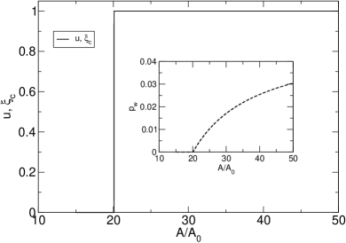
Figure 6: The average composition $u$ and magnetization $\xi_{c}$ are represented as a function of the parameter $A/A_{0}$, for the sharp peak landscape. The mutation rate was set to $\mu=1.0$. Also shown (inset) is the fraction of the population located at the peak, $p_{w}$.

3.5.2 The Fujiyama fitness landscape

We will consider the Fujiyama fitness landscape, which is a linear function of the composition

$$f(\vec{u})=\sum_{i=1}^{3}(\alpha_{i}u_{i})+\alpha_{0}$$ (146)

For the symmetric case, $\alpha_{i}=\alpha$, $\mu_{i}=\mu$. Therefore, we have $\xi_{c}^{1}=\xi_{c}^{2}=\xi_{c}^{3}\equiv\xi_{c}$. The mean fitness, in the absence of degradation, from Eq. (139) becomes

$$f_{m}=\max_{-\frac{1}{3}\leq\xi_{c}\leq 1}\left\{(3\alpha\xi_{c}+\alpha_{0})e^{\frac{3}{2}\mu[-1-\xi_{c}+\sqrt{(1+3\xi_{c})(1-\xi_{c})}]}\right\}$$ (147)

By maximizing with respect to $\xi_{c}$, $\frac{\partial f_{m}}{\partial\xi_{c}}=0$, we obtain the nonlinear equation

$$\alpha-\frac{\mu}{2}\alpha_{0}-\frac{3}{2}\mu\alpha\xi_{c}=\frac{\mu}{2}\frac{(3\alpha\xi_{c}+\alpha_{0})(3\xi_{c}-1)}{\sqrt{(1+3\xi_{c})(1-\xi_{c})}}$$ (148)

No error threshold is observed for this fitness landscape, except for the trivial limit $\alpha\rightarrow 0$, $\alpha_{0}\geq 0$. The average surplus $u$ is obtained by the self-consistent equation

$$f_{m}=3\alpha u+\alpha_{0}$$ (149)

3.6 The quadratic fitness landscape

Next we consider the quadratic fitness landscape

$$f(\vec{u})=\sum_{i=1}^{N}\left(\frac{\beta_{i}}{2}u_{i}^{2}+\alpha_{i}u_{i}\right)+1$$ (150)

For the symmetric case, $\beta_{i}=\beta$, $\alpha_{i}=\alpha$, $\mu_{i}=\mu$, we have $\xi_{c}^{i}=\xi_{c}$ and $\bar{\xi}_{c}^{i}=\bar{\xi}_{c}$. Thus, the mean fitness, for a null degradation rate, after Eq. (139) is

$$f_{m}=\max_{-\frac{1}{3}\leq\xi_{c}\leq 1}\left\{\left(\frac{3}{2}\beta\xi_{c}^{2}+3\alpha\xi_{c}+1\right)e^{\frac{3}{2}\mu[-1-\xi_{c}+\sqrt{(1+3\xi_{c})(1-\xi_{c})}]}\right\}$$ (151)

We maximize with respect to $\xi_{c}$, $\frac{\partial f_{m}}{\partial\xi_{c}}=0$, to obtain

$$\beta\xi_{c}+\alpha=\frac{\mu}{2}\left(\frac{3}{2}\beta\xi_{c}^{2}+3\alpha\xi_{c}+1\right)\left[1+\frac{3\xi_{c}-1}{\sqrt{(1+3\xi_{c})(1-\xi_{c})}}\right]$$ (152)

The average base composition $u$ is obtained from the self-consistent condition

$$f_{m}=f(u)=\frac{3}{2}\beta u^{2}+3\alpha u+1$$ (153)

The selected phase, $\xi_{c}>0$, $u>0$, occurs for $\beta>1.8096\mu$ when $\alpha=0$. The value of $u$ is continuous at the transition, as it can checked from Eq. (151) that $f_{m}(\xi_{c}=0)=f_{m}(\xi_{c}=0.2289,\beta=1.8096,\mu=1)=1$, which implies after Eq. (153) (for $\alpha=0$) that $u=0$ when approaching the critical point $\beta=1.8066\mu$ from both sides. However, $\xi_{c}$ jumps from 0 (for $\beta\rightarrow 1.8066\mu^{-}$) to $0.2289$ (for $\beta\rightarrow 1.8066\mu^{+}$). By expanding Eq. (151) near the critical point, after a similar procedure as in Eq. (84) for the parallel model, we find a discontinuous jump in $df_{m}/d\beta$ from $0$ to $0.06883$. Therefore, the phase transition is of first order in $\beta$. A graphical representation is displayed in Fig. 7.

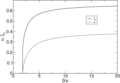
Figure 7: The average composition $u$ and magnetization $\xi_{c}$ are represented as a function of the parameter $\beta/\mu$ for the quadratic fitness,when $\alpha=0$

3.7 The quartic fitness landscape

As a final example, we consider the quartic fitness landscape,

$$f(\vec{u})=\sum_{i=1}^{3}\frac{\beta_{i}}{4}u_{i}^{4}+1$$ (154)

We further consider the symmetric case $\mu_{i}\equiv\mu$, $\beta_{i}\equiv\beta$, and hence $\xi_{c}^{i}\equiv\xi_{c}$. From the general expression Eq. (139), we obtain an analytical expression for the mean fitness

$$f_{m}=\max_{\{-\frac{1}{3}\leq\xi_{c}\leq 1\}}\bigg{\{}\left(\frac{3}{4}\beta\xi_{c}^{4}+1\right)e^{\frac{3}{2}\mu[-1-\xi_{c}+\sqrt{(1+3\xi_{c})(1-\xi_{c})}]}\bigg{\}}$$ (155)

The average composition of the population $u$ is obtained from the self-consistent condition

$$f(u)=\frac{3}{4}\beta u^{4}+1=f_{m}$$ (156)

In Fig. 8, we present the values of $u$ and $\xi_{c}$, as obtained from Eqs. (155), (156), as a function of the parameter $\beta/\mu$. We notice that a discontinuous jump in the bulk magnetization from $\xi_{c}=0$ to $\xi_{c}=0.779856$ is observed at $\beta/\mu=10.776165$. By expanding Eq. (155) near the critical point, we find a discontinuous jump in $df_{m}/d\beta$, from $0$ to $0.066213$. Therefore, the phase transition is of first order in $\beta$. The average composition shows a fast but continuous transition. This behavior is much like the one observed in the sharp peak fitness landscape, Eq. (142), and in the corresponding example for the parallel model.

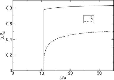
Figure 8: The average composition $u$ and magnetization $\xi_{c}$ are represented as a function of the parameter $\beta/\mu$ for the quartic fitness landscape

3.8 Symmetric case, general h, with application to the amino acid alphabet $h=20$

We consider the case of the amino acid alphabet, which is derived from our general solution Eq. (LABEL:eqGeEig20_1) by setting $h=20$. In particular, when a symmetric mutation scheme is assumed $\mu_{\alpha\beta}=\mu$, for all $\alpha,\beta$, and $x^{\alpha}_{c}=x_{c}$. We first consider the symmetric case for general $h$.

For an alphabet of size $h$, we define a magnetization coordinate $\xi_{c}=1-hx_{c}$, and obtain that Eq. (LABEL:eqGeEig20_1) reduces to

$$f_{m}=\max_{\{-1/(h-1)\leq\xi_{c}\leq 1\}}\bigg{\{}f(\xi_{c})e^{(h-1)\mu[\frac{2}{h}\sqrt{(1-\xi_{c})(1+(h-1)\xi_{c})}+\frac{h-2}{h}(1-\xi_{c})-1]}-d(\xi_{c})\bigg{\}}$$

(157)

As an example of application of Eq. (157), we consider the sharp peak fitness landscape $f(\xi_{c})=(A-A_{0})\delta_{\xi_{c},1}+A_{0}$, and zero degradation function $d(\xi_{c})=0$. Then, from Eq. (157) we obtain the mean fitness

$$f_{m}=\left\{\begin{array}[]{cc}e^{-(h-1)\mu}A,&A>A_{0}e^{(h-1)\mu}\\ A_{0},&A\leq A_{0}e^{(h-1)\mu}\end{array}\right.$$ (160)

The system experiences a first order phase transition at $A_{\rm{crit}}=A_{0}e^{(h-1)\mu}$. The steady-state probability for the wild-type is obtained from the self-consistency condition: $f_{m}=Ap_{w}+A_{0}(1-p_{w})$,

$$p_{w}=\left\{\begin{array}[]{cc}\frac{Ae^{-(h-1)\mu}-A_{0}}{A-A_{0}},&A>A_{0}e^{(h-1)\mu}\\ 0,&A\leq A_{0}e^{(h-1)\mu}\end{array}\right.$$ (163)

The factor $(h-1)\mu$ in the exponential is intuitive, since there exists $h-1$ independent mutation channels into which evolving sequences can escape from the wild-type.

As a second example, we consider the quadratic fitness landscape $f(\xi_{c})=(h-1)\beta\xi_{c}^{2}/2+1$ for an alphabet of size $h$. We consider the case of the amino acid alphabet, with $h=20$. We set $\mu=1$. By a similar analysis as in the parallel model case, we find a phase transition at the critical point $\beta=7.483\mu$. The magnetization parameter $\xi_{c}$ has a finite jump from $\xi_{c}=0$ (for $\beta\rightarrow 7.483\mu^{-}$) to $\xi_{c}=0.0827$ (for $\beta\rightarrow 7.483\mu^{+}$). The mean fitness is continuous at the transition, since $f_{m}(\beta\rightarrow 7.483\mu^{+})=f_{m}(\beta\rightarrow 7.483\mu^{-})=1$, which implies that the observable $u=0$ at the critical point. We observe that the first derivative has a finite jump at the critical point, from $df_{m}/d\beta(\beta\rightarrow 7.483\mu^{-})=0$, to $df_{m}/d\beta(\beta\rightarrow 7.483\mu^{+})=0.0437$, and therefore the phase transition is of first order. A similar analysis shows that the transition is first order for $h=3$ as well. As with the parallel model, we find that the transition for the quadratic fitness function is second order for $h=2$ and first order for $h>2$.

4 Conclusion

Using the quantum spin chain approach, the 2-state, purine/pyrimidine assumption for quasi-species theory has been lifted to arbitrary alphabet sizes $h$. We have here expressed the general result for the fitness of the evolved population as a maximization principle. We have derived the solution for a general fitness function using the Schwinger spin coherent states approach. We have presented analytic results for the sharp peak, as well as linear, quadratic, and quartic fitness functions. For the Kimura 3 ST mutation scheme, we have presented an explicit solution for a general fitness function, expressed as a maximization principle.

We have also derived the general solution to the Eigen model of mutation and selection for arbitrary alphabet size and for a general mutation scheme. We have presented analytic results for the sharp peak, linear, quadratic, and quartic fitness functions.

These results bring quasi-species theory closer to the evolutionary dynamics that occurs at the genetic level.

Appendix 1

In what follows, we will need to apply Euler’s theorem and three properties of the maximum eigenvalue $\lambda_{\rm{max}}$ of the matrix ${\bf{M}}$ defined by Eq. (48).

Euler’s theorem for homogeneous functions

Definition 1: Homogeneous function of degree k

A function $f(x_{1},\ldots,x_{n})$ of $n$ variables is homogeneous of degree $k$ if, for all $\alpha>0$,

$$f(\alpha x_{1},\alpha x_{2},\ldots,\alpha x_{n})=\alpha^{k}f(x_{1},x_{2},\ldots,x_{n})$$ (164)

Euler’s theorem

A differentiable function $f(x_{1},\ldots,x_{n})$ of $n$ variables is homogeneous of degree $k$ if and only if

$$\sum_{i=1}^{n}x_{i}\frac{\partial}{\partial x_{i}}f(x_{1},\ldots,x_{n})=kf(x_{1},\ldots,x_{n})$$ (165)

The theorem and its proof is presented in most textbooks of mathematical analysis [24].

Property I

The maximum eigenvalue $\lambda_{\rm{max}}$ of the matrix ${\bf{M}}$ defined by Eq. (48) is a homogeneous function of degree $k=1$ in the vector $(\bar{x}^{1}_{c},\bar{x}_{c}^{2},\ldots,\bar{x}_{c}^{h-1},\{\mu_{\alpha\beta}\})$.

The proof of this proposition follows directly from Definition 1. Notice that after Eq. (48),

$${\bf{M}}(\{\bar{x}_{c}^{\alpha}\},\{\mu_{\alpha\beta}\})=\sum_{\alpha\neq\beta=1}^{h}\mu_{\alpha\beta}\tau^{\alpha\beta}+\sum_{\alpha=1}^{h-1}\bar{x}^{\alpha}_{c}\Theta^{\alpha}$$

(166)

Since ${\bf{M}}$ is a linear function of the vector $(\bar{x}^{1}_{c},\ldots,\bar{x}^{h-1}_{c},{\mu_{\alpha\beta}})$

$${\bf{M}}(\alpha\bar{x}_{c}^{1},\alpha\bar{x}_{c}^{2},\ldots,\alpha\bar{x}_{c}^{h-1},\alpha\mu_{12},\alpha\mu_{21},\ldots)=\alpha{\bf{M}}(\bar{x}_{c}^{1},\bar{x}_{c}^{2},\ldots,\bar{x}_{c}^{h-1},\mu_{12},\mu_{21},\ldots)$$

(167)

Therefore, the maximum eigenvalue, as obtained from the long-time limit of the trace,

$$\lambda_{\rm{max}}(\alpha\bar{x}_{c}^{1},\alpha\bar{x}_{c}^{2},\ldots,\alpha\bar{x}_{c}^{h-1},\alpha\mu_{12},\alpha\mu_{21},\ldots)$$ (168)

$$= \lim_{t\rightarrow\infty}\frac{1}{t}\ln\bigg{[}{\rm{Tr}}\,e^{t{\bf{M}}(\alpha\bar{x}_{c}^{1},\alpha\bar{x}_{c}^{2},\ldots,\alpha\bar{x}_{c}^{h-1},\alpha\mu_{12},\alpha\mu_{21},\ldots)}\bigg{]}$$

$$= \lim_{t\rightarrow\infty}\frac{1}{t}\ln\bigg{[}{\rm{Tr}}\,e^{t\alpha{\bf{M}}(\bar{x}_{c}^{1},\bar{x}_{c}^{2},\ldots,\bar{x}_{c}^{h-1},\mu_{12},\mu_{21},\ldots)}\bigg{]}$$

$$= \alpha\lambda_{\rm{max}}(\bar{x}_{c}^{1},\bar{x}_{c}^{2},\ldots,\bar{x}_{c}^{h-1},\mu_{12},\mu_{21},\ldots)$$

is also a homogeneous function of degree $k=1$, after Definition 1.

Property II

$\lambda_{\rm{max}}$ satisfies the identity

$$\lambda_{\rm{max}} = \sum_{\alpha=1}^{h-1}\bar{x}^{\alpha}_{c}\frac{\partial\lambda_{\rm{max}}}{\partial\bar{x}^{\alpha}_{c}}+\sum_{\alpha\neq\beta=1}^{h}\mu_{\alpha\beta}\frac{\partial\lambda_{\rm{max}}}{\partial\mu_{\alpha\beta}}$$ (169)

The proof follows directly by application of Euler’s theorem, for a homogeneous function of degree $k=1$.

Notice that, after the saddle-point Eqs. (42)–(45), we have the following identities

$$x_{c}^{\alpha}=\langle\Theta^{\alpha}\rangle = \lim_{t\rightarrow\infty}\frac{{\rm{Tr}}\bigg{[}\Theta^{\alpha}e^{t{\bf{M}}}\bigg{]}}{{\rm{Tr}}\,e^{t{\bf{M}}}}$$ (170)

$$= \lim_{t\rightarrow\infty}\frac{\partial}{\partial\bar{x}_{c}^{\alpha}}\frac{\ln\bigg{[}{\rm{Tr}}\,e^{{t\bf{M}}}\bigg{]}}{t}=\frac{\partial}{\partial\bar{x}_{c}^{\alpha}}\lambda_{{\rm{max}}}$$

$$\langle\tau^{\alpha\beta}\rangle=\frac{\partial}{\partial\mu_{\alpha\beta}}\lambda_{{\rm{max}}}$$ (171)

Substituting Eqs. (170)–(171) into Eq. (169), we obtain the identity

$$\lambda_{{\rm{\max}}}-\sum_{\alpha=1}^{h-1}\bar{x}_{c}^{\alpha}x_{c}^{\alpha}=\sum_{\alpha\neq\beta=1}^{h}\mu_{\alpha\beta}\langle\tau^{\alpha\beta}\rangle$$ (172)

After Eq. (172), Eq. (46) becomes

$$f_{m}=\max_{\{\bar{x}_{c}^{\alpha}\},\{\mu_{\alpha\beta}\}}\bigg{[}f(\{x_{c}^{\alpha}\})-\sum_{\alpha\neq\beta=1}^{h}\mu_{\alpha\beta}(1-\langle\tau^{\alpha\beta}\rangle)\bigg{]}$$

(173)

Property III

The ’average’ $\langle{{\bf{A}}}\rangle$ of an arbitrary $h\times h$ matrix ${{\bf{A}}}$, satisfies the identity

$$\langle{{\bf{A}}}\rangle=\lim_{t\rightarrow\infty}\frac{{\rm{Tr}}\bigg{[}{\bf{A}}\,e^{t{\bf{M}}}\bigg{]}}{{\rm{Tr}}\,e^{t{\bf{M}}}}=\vec{y}_{\rm{max}}^{T}{\bf{A}}\vec{y}_{\rm{max}}$$ (174)

with $\vec{y}_{\rm{max}}$ the eigenvector corresponding to the maximum eigenvalue $\lambda_{\rm{max}}$ of the matrix ${\bf{M}}$ in Eq. (166).

The proof follows by considering the unitary $h\times h$ matrix ${\bf{P}}=[\vec{y}_{1},\vec{y}_{2},\vec{y}_{3},\ldots,\vec{y}_{h}]$, ${\bf{P}}^{-1}={\bf{P}}^{T}$ whose columns are formed by the $h$ orthogonal eigenvectors $\vec{y}_{\alpha}$ of ${\bf{M}}$ which satisfy

$${\bf{M}}\vec{y}_{\alpha} = \lambda_{\alpha}\vec{y}_{\alpha}\,\,\,\,\,1\leq\alpha\leq h$$

$$\vec{y}_{\alpha}\cdot\vec{y}_{\beta} = \delta_{\alpha\beta}$$ (175)

From elementary linear algebra, the matrix ${\bf{P}}$ induces a similarity transformation which diagonalizes ${\bf{M}}$, that is ${\bf{P}}{\bf{M}}{\bf{P}}^{-1}={\rm{diag}}(\lambda_{1},\lambda_{2},\dots,\lambda_{h})\equiv{\bf{D}}$. Hence, it also diagonalizes the exponential of ${\bf{M}}$,

$${\bf{P}}e^{t{\bf{M}}}{\bf{P}}^{-1} = {\bf{P}}({\bf{I}}+t{\bf{M}}+\frac{t^{2}}{2!}{\bf{MM}}+\ldots){\bf{P}}^{-1}$$ (176)

$$= {\bf{I}}+t{\bf{PM}}{\bf{P}}^{-1}+\frac{t^{2}}{2!}{\bf{PM}}{\bf{P}}^{-1}{\bf{PM}}{\bf{P}}^{-1}+\ldots$$

$$= {\bf{I}}+t{\bf{D}}+\frac{t^{2}}{2!}{\bf{D}}^{2}+\ldots$$

$$= e^{t{\bf{D}}}$$

The ’average’ of an arbitrary $h\times h$ matrix ${\bf{A}}$, defined by Eq. (174), is calculated as

$$\langle{\bf{A}}\rangle=\lim_{t\rightarrow\infty}\frac{{\rm{Tr}}\bigg{[}{\bf{A}}\,e^{t{\bf{M}}}\bigg{]}}{{\rm{Tr}}\,e^{t{\bf{M}}}} = \lim_{t\rightarrow\infty}\frac{{\rm{Tr}}\bigg{[}{\bf{PA}}{\bf{P}}^{-1}{\bf{P}}e^{t{\bf{M}}}{\bf{P}}^{-1}\bigg{]}}{{\rm{Tr}}\bigg{[}{\bf{P}}e^{t{\bf{M}}}{\bf{P}}^{-1}\bigg{]}}$$ (177)

$$= \lim_{t\rightarrow\infty}\frac{{\rm{Tr}}\bigg{[}{\bf{PA}}{\bf{P}}^{-1}e^{t{\bf{D}}}\bigg{]}}{{\rm{Tr}}\,e^{t{\bf{D}}}}$$

$$= \lim_{t\rightarrow\infty}\frac{\sum_{i=1}^{h}\vec{y}_{i}^{T}{\bf{A}}\vec{y}_{i}e^{t\lambda_{i}}}{\sum_{j=1}^{h}e^{t\lambda_{j}}}=\vec{y}_{{\rm{max}}}^{T}{\bf{A}}\vec{y}_{{\rm{max}}}$$

which proves the Property III.

We can express the eigenvector $\vec{y}_{\rm{max}}=(y^{1},y^{2},\ldots,y^{h})^{T}$ in terms of the fields $x_{c}^{\alpha}$, by combining the result in Property III, with the saddle-point equations Eq. (170),(171), as follows

$$x_{c}^{\alpha} = \langle\Theta^{\alpha}\rangle=\vec{y}_{{\rm{max}}}^{T}\Theta^{\alpha}\vec{y}_{{\rm{max}}}$$ (178)

$$= (y^{\alpha})^{2}$$

These equations are inverted to obtain

$$y^{\alpha}=\left\{\begin{array}[]{cc}\sqrt{x^{\alpha}_{c}},&1\leq\alpha\leq h-1\\ \sqrt{1-\sum_{\gamma=1}^{h-1}x^{\gamma}_{c}},&\alpha=h\end{array}\right.$$ (181)

Equipped with this result, we can now calculate the ’averages’ $\langle\tau^{\alpha\beta}\rangle$ in Eq. (173),

$$\langle\tau^{\alpha\beta}\rangle = \vec{y}_{\rm{max}}^{T}\tau^{\alpha\beta}\vec{y}_{\rm{max}}$$ (182)

$$= y^{\alpha}y^{\beta}+\sum_{\gamma\neq\alpha}(y^{\gamma})^{2}$$

Substituting Eq. (181) into Eq. (182), we obtain the result

$$\langle\tau^{\alpha\beta}\rangle=\left\{\begin{array}[]{cc}\sqrt{x^{\alpha}_{c}x^{\beta}_{c}}+1-x^{\alpha}_{c},&\alpha\neq\beta\neq h\\ \sqrt{x^{\alpha}_{c}\left(1-\sum_{\gamma=1}^{h-1}x^{\gamma}_{c}\right)}+1-x^{\alpha}_{c},&\beta=h,\,\alpha\neq h\\ \sqrt{\left(1-\sum_{\gamma=1}^{h-1}x^{\gamma}_{c}\right)x^{\beta}_{c}}+\sum_{\gamma=1}^{h-1}x^{\gamma}_{c},&\alpha=h,\,\beta\neq h\end{array}\right.$$ (186)

Substituting Eq. (186) into Eq. (173), we obtain the final solution for the mean fitness of the parallel model in an alphabet of size $h$, with an arbitrary mutation scheme,

$$f_{m}^{(h)} = \max_{\{x^{1}_{c},x^{2}_{c},\ldots,x^{h-1}_{c}\}}\bigg{\{}f(x^{1}_{c},x^{2}_{c},\ldots,x^{h-1}_{c})+\sum_{\alpha\neq\beta=1}^{h-1}\mu_{\alpha\beta}\left[\sqrt{x^{\alpha}_{c}x^{\beta}_{c}}-x^{\alpha}_{c}\right]$$ (187)

$$+\sum_{\alpha=1}^{h-1}\mu_{\alpha h}\left[\sqrt{x^{\alpha}_{c}\left(1-\sum_{\gamma=1}^{h-1}x^{\gamma}_{c}\right)}-x^{\alpha}_{c}\right]$$

$$+\sum_{\beta=1}^{h-1}\mu_{h\beta}\left[\sqrt{\left(1-\sum_{\gamma=1}^{h-1}x^{\gamma}_{c}\right)x^{\beta}_{c}}+\sum_{\gamma=1}^{h-1}x^{\gamma}_{c}-1\right]\bigg{\}}$$

Appendix 2

By performing elementary algebraic manipulations Eq. (79)

$$3\beta\xi_{c}+3\alpha-\frac{3}{2}\mu+\frac{3}{2}\frac{2-6\xi_{c}}{2\sqrt{1+2\xi_{c}-3\xi_{c}^{2}}}=0$$

can be cast into the standard form of a quartic equation

$$A\xi_{c}^{4}+B\xi_{c}^{3}+C\xi_{c}^{2}+D\xi_{c}+E=0$$ (188)

where, by defining $\tilde{\mu}\equiv\mu/\beta$ and $\tilde{\alpha}\equiv\alpha/\beta$, the coefficients correspond to

$$A = 3$$

$$B = 6\tilde{\alpha}-3\tilde{\mu}-2$$ (189)

$$C = 3\tilde{\mu}^{2}-3\tilde{\alpha}\tilde{\mu}+3\tilde{\alpha}^{2}+2\tilde{\mu}-4\tilde{\alpha}-1$$

$$D = -2\tilde{\alpha}-2\tilde{\alpha}^{2}+\tilde{\mu}+2\tilde{\alpha}\tilde{\mu}-2\tilde{\mu}^{2}$$

$$E = -\tilde{\alpha}^{2}+\tilde{\alpha}\tilde{\mu}$$ (190)

We remark that this quartic equation introduces additional, unphysical solutions to the original Eq. (79). However, discarding these unphysical solutions whenever appropriate, the quartic Eq. (188) allows us to obtain explicit analytical expressions for $\xi_{c}$ in the entire region of parameters. Following Ferrari’s method [25], we define the parameters

$$a_{1} = -\frac{3B^{2}}{8A^{2}}+\frac{C}{A}$$ (191)

$$= -\frac{1}{2}-\frac{\tilde{\alpha}}{3}-\frac{\tilde{\alpha}^{2}}{2}+\frac{\tilde{\mu}}{6}+\frac{\tilde{\alpha}\tilde{\mu}}{2}+\frac{5\tilde{\mu}^{2}}{8}$$

$$a_{2} = \frac{B^{3}}{8A^{3}}-\frac{BC}{2A^{2}}+\frac{D}{A}$$ (192)

$$= -\frac{4}{27}-\frac{4\tilde{\alpha}}{9}+\frac{2\tilde{\mu}}{9}-\frac{\tilde{\mu}^{2}}{4}-\frac{3\tilde{\alpha}\tilde{\mu}^{2}}{4}+\frac{3\tilde{\mu}^{3}}{8}$$

$$a_{3} = -\frac{3B^{4}}{256A^{4}}+\frac{CB^{2}}{16A^{3}}-\frac{BD}{4A^{2}}+\frac{E}{A}$$ (193)

$$= -\frac{5}{432}-\frac{7\tilde{\alpha}}{108}-\frac{5\tilde{\alpha}^{2}}{72}+\frac{\tilde{\alpha}^{3}}{12}+\frac{\tilde{\alpha}^{4}}{16}+\frac{7\tilde{\mu}}{216}+\frac{5\tilde{\alpha}\tilde{\mu}}{72}-\frac{\tilde{\alpha}^{2}\tilde{\mu}}{8}-\frac{\tilde{\alpha}^{3}\tilde{\mu}}{8}+\frac{\tilde{\mu}^{2}}{288}$$

$$+\frac{3\tilde{\alpha}\tilde{\mu}^{2}}{16}+\frac{9\tilde{\alpha}^{2}\tilde{\mu}^{2}}{32}-\frac{7\tilde{\mu}^{3}}{96}-\frac{7\tilde{\alpha}\tilde{\mu}^{3}}{32}+\frac{13\tilde{\mu}^{4}}{256}$$

and solve the depressed quartic equation in the auxiliary variable $z=\xi_{c}+B/4A$,

$$z^{4}+a_{1}z^{2}+a_{2}z+a_{3}=0$$ (194)

We analyze the different cases in the parameter space that defines the possible solutions of this equation.

Case 1: $a_{2}=0$. This situation arises at the critical value

$$\tilde{\mu}_{c}^{(1)}=\frac{2}{3}+2\tilde{\alpha}$$ (195)

We obtain four possible roots, according to the general formula

$$\xi_{c} = -\frac{B}{4A}\pm\sqrt{\frac{-a_{1}\pm\sqrt{a_{1}^{2}-4a_{3}}}{2}}$$ (196)

$$= \frac{1}{6}\left(2\pm\sqrt{2}\sqrt{1-9\tilde{\alpha}(2+3\tilde{\alpha})\pm|1-9\tilde{\alpha}(2+3\alpha)|}\right)$$

Depending on the sign of the term in the square root, we have the following solutions

i) If $1-18\tilde{\alpha}-27\tilde{\alpha}^{2}>0$. This situation occurs when $-\frac{1}{3}\leq\tilde{\alpha}\leq\frac{1}{3}\left(\sqrt{\frac{4}{3}}-1\right)$, and the solution is

$$\xi_{c,\pm}=\frac{1}{3}(1\pm\sqrt{1-18\tilde{\alpha}-27\tilde{\alpha}^{2}}), \>\xi_{c}=\frac{1}{3}$$ (197)

ii) If $1-18\tilde{\alpha}-27\tilde{\alpha}^{2}\leq 0$. This situation occurs when $\tilde{\alpha}>\frac{1}{3}\left(\sqrt{\frac{4}{3}}-1\right)$.

$$\xi_{c}=\frac{1}{3}$$ (198)

We shall consider $\tilde{\alpha}\geq 0$ in the region of physically meaningful parameters. When $\tilde{\alpha}=0$, a non-selective phase is obtained, from Eq. (197), if $\beta<\frac{3}{2}\mu$. At $\beta=\frac{3}{2}\mu$, for $\alpha=0$, a finite ’jump’ in the value of $\xi_{c}$ from 0 to 2/3 defines a phase transition, where the value of u varies continuously from 0 to a positive value.

When $0\leq\tilde{\alpha}\leq\frac{1}{3}\left(\sqrt{\frac{4}{3}}-1\right)$, a finite jump in the bulk magnetization from $\xi_{c,-}$ to $\xi_{c,+}$ is observed. This result is in agreement with [15].

Case 2: $a_{3}=0$, $a_{2}\neq 0$. This situation occurs at the critical values

$$\tilde{\mu}_{c}^{(2)}=\frac{2}{39}\left(1+3\tilde{\alpha}+2\sqrt{49-18\tilde{\alpha}-27\tilde{\alpha}^{2}}\right), 0\leq\tilde{\alpha}\leq 1.054444$$ (199)

$$\tilde{\mu}_{c}^{(3)}=\frac{2}{39}\left(1+3\tilde{\alpha}-2\sqrt{49-18\tilde{\alpha}-27\tilde{\alpha}^{2}}\right), 1\leq\tilde{\alpha}\leq 1.054444$$ (200)

In this case, the quartic equation in $z$ factorizes,

$$z(z^{3}+a_{1}z+a_{2})=0$$ (201)

There is a solution $z=0$ for Eq. (201). This is however not a solution of Eq. (79), but an artifact of introducing the algebraic transformation into the fourth order polynomial Eq. (188).

The solutions corresponding to the remaining cubic equation in Eq. (201) are analyzed as follows. Let us define the parameters,

$$s_{1}=\left[-\frac{a_{2}}{2}+\left(\frac{a_{1}^{3}}{27}+\frac{a_{2}^{2}}{4}\right)^{1/2}\right]^{1/3}$$

$$s_{2}=\left[-\frac{a_{2}}{2}-\left(\frac{a_{1}^{3}}{27}+\frac{a_{2}^{2}}{4}\right)^{1/2}\right]^{1/3}$$ (202)

Then, we have the following cases,

Case 2.a: Consider $\tilde{\mu}=\tilde{\mu}_{c}^{(2)}$, defined by Eq. (199). This situation is possible when $0\leq\tilde{\alpha}\leq 1.054444$. Within this range of values for $\tilde{\alpha}$, the parameter $\frac{a_{1}^{3}}{27}+\frac{a_{2}^{2}}{4}\geq 0$. Then, we find a single real solution

$$\xi_{c}=\frac{1}{39}\left(7-18\tilde{\alpha}+\sqrt{49-18\tilde{\alpha}-27\tilde{\alpha}^{2}}\right)+s_{1}+s_{2}$$ (203)

Case 2.b: Consider $\tilde{\mu}=\tilde{\mu}_{c}^{(3)}$, defined by Eq. (200). This situation is possible when $1\leq\tilde{\alpha}\leq 1.054444$. Within this range of values for $\tilde{\alpha}$, the parameter $\frac{a_{1}^{3}}{27}+\frac{a_{2}^{2}}{4}\geq 0$. Then, we find a single real solution

$$\xi_{c}=\frac{1}{39}\left(7-18\tilde{\alpha}-\sqrt{49-18\tilde{\alpha}-27\tilde{\alpha}^{2}}\right)+s_{1}+s_{2}$$ (204)

Case 3: $a_{3}\neq 0$, $a_{2}\neq 0$. In this case, we consider again the general quartic Eq. (188). Following Ferrari’s method [25], we find 4 possible roots

$$\xi_{c,(1,2)}=-\frac{B}{4A}+\frac{1}{2}P\pm\frac{1}{2}Q$$

$$\xi_{c,(3,4)}=-\frac{B}{4A}-\frac{1}{2}P\pm\frac{1}{2}U$$ (205)

Here, we defined

$$P=\sqrt{\frac{B^{2}}{4A^{2}}-\frac{C}{A}+y_{1}}$$ (206)

$$Q=\left\{\begin{array}[]{cc}\sqrt{\frac{3}{4}\frac{B^{2}}{A^{2}}-P^{2}-2\frac{C}{A}+\frac{1}{4}(4\frac{BC}{A^{2}}-8\frac{D}{A}-\frac{B^{3}}{A^{3}})P^{-1}},&P\neq 0\\ \sqrt{\frac{3}{4}\frac{B^{2}}{A^{2}}-2\frac{C}{A}+2\sqrt{y_{1}^{2}-4\frac{E}{A}}},&P=0\end{array}\right.$$ (209)

$$U=\left\{\begin{array}[]{cc}\sqrt{\frac{3}{4}\frac{B^{2}}{A^{2}}-P^{2}-2\frac{C}{A}-\frac{1}{4}(4\frac{BC}{A^{2}}-8\frac{D}{A}-\frac{B^{3}}{A^{3}})P^{-1}},&P\neq 0\\ \sqrt{\frac{3}{4}\frac{B^{2}}{A^{2}}-2\frac{C}{A}-2\sqrt{y_{1}^{2}-4\frac{E}{A}}},&P=0\end{array}\right.$$ (212)

From Eq. (205), the largest real root corresponds to the physical solution of Eq. (79).

The parameter $y_{1}$ in Eqs. (206–212) is obtained as the real root of the auxiliary cubic equation

$$y^{3}+\gamma_{2}y^{2}+\gamma_{1}y+\gamma_{0}=0$$ (213)

Here, we defined the parameters

$$\gamma_{2} = -\frac{C}{A}$$

$$\gamma_{1} = \frac{BD}{A^{2}}-4\frac{E}{A}$$

$$\gamma_{0} = 4\frac{CE}{A^{2}}-\frac{D^{2}}{A^{2}}-\frac{B^{2}E}{A^{3}}$$ (214)

Let us define

$$q = \frac{\gamma_{1}}{3}-\frac{\gamma_{2}^{2}}{9}$$

$$r = \frac{1}{6}(\gamma_{1}\gamma_{2}-3\gamma_{0})-\frac{\gamma_{2}^{3}}{27}$$

$$\Delta = q^{3}+r^{2}$$ (215)

We have three possible cases: $\Delta>0$, $\Delta=0$, and $\Delta<0$.

Case 3.a: $\Delta>0$. In this case, we have one real root $y_{1}$ for the auxiliary cubic Eq. (213), and two complex roots. The real root to be used in Eqs. (205–212) is given by

$$y_{1}=(r+\Delta^{1/2})^{1/3}+(r-\Delta^{1/2})^{1/3}-\frac{\gamma_{2}}{3}$$ (216)

Case 3.b: $\Delta=0$. In this case, all roots of the auxiliary cubic Eq. (213) are real, with two of them identical, and given by

$$y_{1} = 2r^{1/3}-\frac{\gamma_{2}}{3}$$

$$y_{2} = y_{3}=-r^{1/3}$$ (217)

In this case, we take the root $y_{1}$ in Eq. (217), to be used in the formulas Eqs. (205–212).

Case 3.c: $\Delta<0$. In this case, all three roots of the auxiliary cubic Eq. (213) are real and different.

$$y_{1} = 2(r^{2}-\Delta)^{1/6}\cos(\theta/3)-\frac{\gamma_{2}}{3}$$

$$y_{2} = -2(r^{2}-\Delta)^{1/6}\cos(\theta/3+\pi/3)-\frac{\gamma_{2}}{3}$$

$$y_{3} = -2(r^{2}-\Delta)^{1/6}\cos(\theta/3-\pi/3)-\frac{\gamma_{2}}{3}$$ (218)

Here, $\theta=\tan^{-1}\left(\frac{(-\Delta)^{1/2}}{r}\right)$. We take the root $y_{1}$ to be used in Eqs. (205–212).

Appendix 3

The same arguments based on the homogeneous property of $\lambda_{\rm{max}}$ and application of Euler’s theorem can be repeated for the case of the Eigen model, to obtain a solution for the non-symmetric case, starting from Eq. (LABEL:eq108b). Now, the matrix to consider is

$${\bf{M}}(\{\bar{x}_{c}^{\alpha}\},\{\bar{\eta}^{\alpha\beta}\})=\sum_{\alpha\neq\beta=1}^{h}\bar{\eta}_{c}^{\alpha\beta}\tau^{\alpha\beta}+\sum_{\alpha=1}^{h-1}\bar{x}_{c}^{\alpha}\Theta^{\alpha}$$ (219)

Since ${\bf{M}}$ is clearly a homogeneous function of degree $k=1$ in the vector $(\bar{x}_{c}^{1},\bar{x}_{c}^{2},\ldots,\bar{x}_{c}^{h-1},\{\eta^{\alpha\beta}_{c}\})$, $\lambda_{{\rm{max}}}$ is homogeneous of degree $k=1$ as well (the proof is identical as in Property I, Appendix 1 for the parallel model). Therefore, after Euler’s theorem (see Appendix 1), we have the identity

$$\lambda_{{\rm{max}}}-\sum_{\alpha=1}^{h-1}\bar{x}^{\alpha}_{c}x^{\alpha}_{c}-\sum_{\alpha\neq\beta=1}^{h}\bar{\eta}_{c}^{\alpha\beta}\eta_{c}^{\alpha\beta}=0$$ (220)

After the saddle-point Eqs. (129)–(130), we obtain the same components for the eigenvalue $\vec{y}_{\rm{max}}$ as in the parallel case, Eq. (182),

$$y^{\alpha}=\left\{\begin{array}[]{cc}\sqrt{x^{\alpha}_{c}},&1\leq\alpha\leq h-1\\ \sqrt{1-\sum_{\gamma=1}^{h-1}x^{\gamma}_{c}},&\alpha=h\end{array}\right.$$ (223)

Thus, by applying Property III (Appendix 1) for the Eigen model, we obtain

$$\eta_{c}^{\alpha\beta} = \langle\tau^{\alpha\beta}\rangle=\vec{y}_{\rm{max}}^{T}\tau^{\alpha\beta}\vec{y}_{\rm{max}}$$ (227)

$$= \left\{\begin{array}[]{cc}\sqrt{x^{\alpha}_{c}x^{\beta}_{c}}+1-x^{\alpha}_{c},&\alpha\neq\beta\neq h\\ \sqrt{x^{\alpha}_{c}\left(1-\sum_{\gamma=1}^{h-1}x^{\gamma}_{c}\right)}+1-x^{\alpha}_{c},&\beta=h,\,\alpha\neq h\\ \sqrt{\left(1-\sum_{\gamma=1}^{h-1}x^{\gamma}_{c}\right)x^{\beta}_{c}}+\sum_{\gamma=1}^{h-1}x^{\gamma}_{c},&\alpha=h,\,\beta\neq h\end{array}\right.$$

Thus, the mean fitness for the $h$-states Eigen model under arbitrary mutation scheme is given by the expression

$$f_{m} = \max_{\{x^{1}_{c},x^{2}_{c},\ldots,x^{h-1}_{c}\}}\bigg{\{}f(x^{1}_{c},x^{2}_{c},\ldots,x^{h-1}_{c})e^{\sum_{\alpha\neq\beta=1}^{h-1}\mu_{\alpha\beta}[\sqrt{x^{\alpha}_{c}x^{\beta}_{c}}-x^{\alpha}_{c}]}$$ (228)

$$\times e^{\sum_{\alpha=1}^{h-1}\mu_{\alpha h}[\sqrt{x^{\alpha}_{c}\left(1-\sum_{\gamma=1}^{h-1}x^{\gamma}_{c}\right)}-x^{\alpha}_{c}]+\sum_{\beta=1}^{h-1}\mu_{h\beta}[\sqrt{\left(1-\sum_{\gamma=1}^{h-1}x^{\gamma}_{c}\right)x^{\beta}_{c}}+\sum_{\gamma=1}^{h-1}x^{\gamma}_{c}-1]}$$

$$-d(x^{1}_{c},x^{2}_{c},\ldots,x^{h-1}_{c})\bigg{\}}$$

References

[1]
M. Eigen and P. Schuster.
Selforganization of matter and evolution of biological
macromolecules.
Naturwissenschaften, 58:465, 1971.
[2]
M. Eigen, J. McCaskill, and P. Schuster.
Molecular quasi-species.
J. Phys. Chem., 92:6881–16891, 1988.
[3]
M. Eigen, J. McCaskill, and P. Schuster.
The molecular quasi-species.
Adv.Chem.Phys., 75:149–263, 1989.
[4]
J. Crow and M. Kimura.
An introduction to population genetics theory.
Harper and Row, New York, 1970.
[5]
C. K. Biebricher and M. Eigen.
The error threshold.
Virus Res., 107:117–127, 2005.
[6]
E. Domingo, D. Sabo, T. Taniguchi, and C. Weissman.
Nucleotide sequence heterogeneity of an RNA phage population.
Cell, 13:735–744, 1978.
[7]
E. Domingo, C. Escarmis, E. Lazaro, and S. C. Manrubia.
Quasispecies dynamics and RNA virus extinction.
Virus Res., 107:129–139, 2005.
[8]
I. Leuthausser.
Statistical mechanics of Eigen’s evolution model.
J. Stat. Mech.: Theor. Exp., 48:343–360, 1987.
[9]
P. Tarazona.
Error thresholds for molecular quasispecies as phase transitions:
From simple landscapes to spin-glass models.
Phys. Rev. A, 45:6038–6050, 1992.
[10]
E. Baake, M. Baake, and H. Wagner.
Ising quantum chain is equivalent to a model for biological
evolution.
Phys. Rev. Lett., 78:559–562, 1997.
[11]
E. Baake, M. Baake, and H. Wagner.
Quantum mechanics versus classical probability in biological
evolution.
Phys. Rev. E, 57:1191–1192, 1998.
[12]
E. Baake and H. Wagner.
Mutation-selection models solved exactly with methods of statistical
mechanics.
Genet. Res. Camb., 78:93–117, 2001.
[13]
D. B. Saakian and C.-K. Hu.
Eigen model as a quantum spin chain: Exact dynamics.
Phys. Rev. E, 70:021913, 2004.
[14]
D. B. Saakian, E. Muñoz, C.-K. Hu, and M. W. Deem.
Quasispecies theory for multiple-peak fitness landscapes.
Phys. Rev. E, 73:041913, 2006.
[15]
J. Hermisson, H. Wagner, and M. Baake.
Four-state quantum chain as a model for sequence evolution.
J. Stat. Phys., 102:315–343, 2001.
[16]
T. Garske and U. Grimm.
A maximum principle for the mutation-selection equilibrium of
nucleotide sequences.
Bull. Math. Biol., 66:397–421, 2004.
[17]
T. Garske and U Grimm.
Maximum principle and mutation thresholds for four-letter sequence
evolution.
J. Stat. Mech.: Theor. Exp., P07007, 2004.
[18]
E. Baake, M. Baake, A. Bovier, and M. Klein.
An asymptotic maximum principle for essentially linear evolution
models.
J. Math. Biol., 50:83–114, 2005.
[19]
J.-M. Park and M. W. Deem.
Schwinger boson formulation and solution of the Crow-Kimura and
Eigen models of quasispecies theory.
J. Stat. Phys., 125:975–1015, 2006.
[20]
J.-M. Park and M. W. Deem.
Phase diagrams of quasispecies theory with recombination and
horizontal gene transfer.
Phys. Rev. Lett., 98:05101, 2007.
[21]
E. Muñoz, J.-M. Park, and M. W. Deem.
Quasispecies theory for horizontal gene transfer and recombination.
Phys. Rev. E, 78:061921, 2008.
[22]
M. Kimura.
Estimation of evolutionary distances between homologous nucleotide
sequences.
Proc. Natl. Acad. Sci. USA, 78:454–458, 1981.
[23]
J. Hermisson, O. Redner, H. Wagner, and E. Baake.
Mutation-selection balance: Ancestry, load, and maximum principle.
Theor. Pop. Biol., 62:9–42, 2002.
[24]
Fritz John.
Partial differential equations.
Springer, 4th edition, 1982.
[25]
M. Abramowitz and I. A. Stegun.
Handbook of mathematical functions.
Dover, New York, 1970.