Feature selection in omics prediction problems using cat scores and false nondiscovery rate control

Abstract

We revisit the problem of feature selection in linear discriminant analysis (LDA), that is, when features are correlated. First, we introduce a pooled centroids formulation of the multiclass LDA predictor function, in which the relative weights of Mahalanobis-transformed predictors are given by correlation-adjusted $t$-scores (cat scores). Second, for feature selection we propose thresholding cat scores by controlling false nondiscovery rates (FNDR). Third, training of the classifier is based on James–Stein shrinkage estimates of correlations and variances, where regularization parameters are chosen analytically without resampling. Overall, this results in an effective and computationally inexpensive framework for high-dimensional prediction with natural feature selection. The proposed shrinkage discriminant procedures are implemented in the R package “sda” available from the R repository CRAN.

and Miika Ahdesmaki, Korbinian Strimmer

1 Introduction

Class prediction of biological samples based on their genetic or proteomic profile is now a routine task in genomic studies. Accordingly, many classification methods have been developed to address the specific statistical challenges presented by these data—see, for example, Schwender, Ickstadt and Rahnenführer (2008) and Slawski, Daumer and Boulesteix (2008) for recent reviews. In particular, the small sample size $n$ renders difficult the training of the classifier, and the large number of variables $p$ makes it hard to select suitable features for prediction.

Perhaps surprisingly, despite the many recent innovations in the field of classification methodology, including the introduction of sophisticated algorithms for support vector machines and the proposal of ensemble methods such as random forests, the conceptually simple approach of linear discriminant analysis (LDA) and its sibling, diagonal discriminant analysis (DDA), remain among the most effective procedures also in the domain of high-dimensional prediction [Efron (2008a); Hand (2006); Efron (1975)].

In order to be applicable for high-dimensional analysis, it has been recognized early that regularization is essential [Friedman (1989)]. Specifically, when training the classifier, that is, when estimating the parameters of the discriminant function from training data, particular care needs to be taken to accurately infer the (inverse) covariance matrix. A rather radical, yet highly effective way to regularize covariance estimation in high dimensions is to set all correlations equal to zero [Bickel and Levina (2004)]. Employing a diagonal covariance matrix reduces LDA to the special case of diagonal discriminant analysis (DDA), also known in the machine learning community as “naive Bayes” classification.

In addition to facilitating high-dimensional estimation of the prediction function, DDA has one further key advantage: it is straightforward to conduct feature selection. In the DDA setting with two classes ($K=2$), it can be shown that the optimal criterion for ordering features relevant for prediction are the $t$-scores between the two group means [e.g., Fan and Fan (2008)], or in the multiclass setting, the $t$-scores between group means and the overall centroid.

The nearest shrunken centroids (NSC) algorithm [Tibshirani et al. (2002, 2003)], commonly known by the name of “PAM” after its software implementation, is a regularized version of DDA with multiclass feature selection. The fact that PAM has established itself as one of the most popular methods for classification of gene expression data is ample proof that DDA-type procedures are indeed very effective for large-scale prediction problems—see also Bickel and Levina (2004) and Efron (2008a).

However, there are now many omics data sets where correlation among predictors is an essential feature of the data and hence cannot easily be ignored. For example, this includes proteomics, imaging, and metabolomics data where correlation among biomarkers is commonplace and induced by spatial dependencies and by chemical similarities, respectively. Furthermore, in many transcriptome measurements there are correlations among genes within a functional group or pathway [Ackermann and Strimmer (2009)].

Consequently, there have been several suggestions to generalize PAM to account for correlation. This includes the SCRDA [Guo, Hastie and Tibshirani (2007)], Clanc [Dabney and Storey (2007)] and MLDA [Xu, Brock and Parrish (2009)] approaches. All these methods are regularized versions of LDA, and hence offer automatic provisions for gene-wise correlations. However, in contrast to PAM and DDA, they lack an efficient and elegant feature selection scheme, due to problems with multiple optima in the choice of regularization parameters (SCRDA) and the large search space for optimal feature subsets (Clanc).

In this paper we present a framework for efficient high-dimensional LDA analysis. This is based on three cornerstones. First, we employ James–Stein shrinkage rules for training the classifier. All regularization parameters are estimated from the data in an analytic fashion without resorting to computationally expensive resampling. Second, we use correlation-adjusted $t$-scores (cat scores) for feature selection. These scores emerge from a restructured version of the LDA equations and enable simple and effective ranking of genes even in the presence of correlation. Third, we employ false nondiscovery rate thresholding for selecting features for inclusion in the prediction rule. As we will show below, this is a highly effective method with similar performance to the recently proposed “higher criticism” approach.

The remainder of the paper is organized as follows. In Sections 2–5 we detail our framework for shrinkage discriminant analysis and variable selection. Subsequently, we demonstrate the effectiveness of our approach by application to a number of high-dimensional genomic data sets. We conclude with a discussion and comparison to closely related approaches.

2 Linear discriminant analysis revisited

2.1 Standard formulation

LDA starts by assuming a mixture model for the $p$-dimensional data $\mathbf{x}$,

$$f(\mathbf{x})=\sum_{j=1}^{K}\pi_{j}f(\mathbf{x}|j),$$

where each of the $K$ classes is represented by a multivariate normal density

$$f(\mathbf{x}|k)=(2\pi)^{-p/2}|\bolds{\Sigma}|^{-1/2}\exp\bigl{\{}-\tfrac{1}{2}(\mathbf{x}-\bolds{\mu}_{k})^{T}\bolds{\Sigma}^{-1}(\mathbf{x}-\bolds{\mu}_{k})\bigr{\}}$$

with group-specific centroids $\bolds{\mu}_{k}$ and a common covariance matrix $\bolds{\Sigma}$. The probability of group $k$ given $\mathbf{x}$ is computed from the a priori mixing weights $\pi_{j}$ by application of Bayes’ theorem,

$$\operatorname{Pr}(k|\mathbf{x})=\frac{\pi_{k}f(\mathbf{x}|k)}{f(\mathbf{x})}.$$

We define here the LDA discriminant score as the log posterior $d_{k}(\mathbf{x})=\break\log\{\operatorname{Pr}(k|\mathbf{x})\}$, which after dropping terms constant across groups becomes

$$d_{k}^{\mathrm{LDA}}(\mathbf{x})=\bolds{\mu}_{k}^{T}\bolds{\Sigma}^{-1}\mathbf{x}-\tfrac{1}{2}\bolds{\mu}_{k}^{T}\bolds{\Sigma}^{-1}\bolds{\mu}_{k}+\log(\pi_{k}).$$ (1)

Due to the common covariance, $d_{k}^{\mathrm{LDA}}(\mathbf{x})$ is linear in $\mathbf{x}$. Prediction in LDA works by evaluating the discriminant function at the given test sample $\mathbf{x}$ for all possible $k$, choosing the class maximizing the posterior probability (and hence $d_{k}^{\mathrm{LDA}}$).

2.2 Pooled centroid formulation

We now rewrite the standard form of the LDA predictor function (1) with the aim to elucidate the influence of each individual variable in prediction. Specifically, we simply add a class-independent constant to the discriminant function—note that this does not change in any way the prediction. We compute the pooled mean

$$\bolds{\mu}_{\mathrm{pool}}=\sum_{j=1}^{K}\frac{n_{j}}{n}\bolds{\mu}_{j},$$

representing the overall centroid ($n_{j}$ is the sample size in group $j$ and $n=\sum_{j=1}^{K}n_{j}$ the total number of observations) and the corresponding discriminant score

$$d_{\mathrm{pool}}^{\mathrm{LDA}}(\mathbf{x})=\bolds{\mu}_{\mathrm{pool}}^{T}\bolds{\Sigma}^{-1}\mathbf{x}-\tfrac{1}{2}\bolds{\mu}_{\mathrm{pool}}^{T}\bolds{\Sigma}^{-1}\bolds{\mu}_{\mathrm{pool}}.$$

The centered score

$$\Delta_{k}^{\mathrm{LDA}}(\mathbf{x})=d_{k}^{\mathrm{LDA}}(\mathbf{x})-d_{\mathrm{pool}}^{\mathrm{LDA}}(\mathbf{x})$$

can be interpreted as a log posterior ratio and is, in terms of prediction, completely equivalent to the original $d_{k}^{\mathrm{LDA}}(\mathbf{x})$. After some careful algebra, it simplifies to

$$\Delta_{k}^{\mathrm{LDA}}(\mathbf{x})=\bolds{\omega}_{k}^{T}\bolds{\delta}_{k}(\mathbf{x})+\log(\pi_{k})$$ (2)

with feature weight vector

$$\bolds{\omega}_{k}=\mathbf{P}^{-1/2}\mathbf{V}^{-1/2}(\bolds{\mu}_{k}-\bolds{\mu}_{\mathrm{pool}})$$ (3)

and Mahalanobis-transformed predictors

$$\bolds{\delta}_{k}(\mathbf{x})=\mathbf{P}^{-1/2}\mathbf{V}^{-1/2}\biggl{(}\mathbf{x}-\frac{\bolds{\mu}_{k}+\bolds{\mu}_{\mathrm{pool}}}{2}\biggr{)}.$$ (4)

Here, we have made use of the variance-correlation decomposition of the covariance matrix $\bolds{\Sigma}=\mathbf{V}^{1/2}\mathbf{P}\mathbf{V}^{1/2}$, where $\mathbf{V}=\operatorname{diag}\{\sigma^{2}_{1},\ldots,\sigma^{2}_{p}\}$ is a diagonal matrix containing the variances and $\mathbf{P}=(\rho_{ij})$ is the correlation matrix.

A remarkable property of the above restructuring (2)–(4) of the LDA discriminant function (1) is that both $\bolds{\omega}_{k}$ and $\bolds{\delta}_{k}(\mathbf{x})$ are vectors and not matrices. Furthermore, note that $\bolds{\omega}_{k}$ is not a function of the test data $\mathbf{x}$ and that its components control how much each individual variable contributes to the score $\Delta_{k}^{\mathrm{LDA}}$ of group $k$.

2.3 James–Stein shrinkage rules for learning the LDA predictor

In order to train the LDA discriminant function [(1) or (2)], we estimate group centroids $\bolds{\mu}_{k}$ by their empirical means, and otherwise rely on three different James–Stein-type shrinkage rules. Specifically, we employ the following:

1. for the correlations $\mathbf{P}$ the ridge-type estimator from Schäfer and Strimmer (2005),

2. for the variances $\mathbf{V}$ the shrinkage estimator from Opgen-Rhein and Strimmer (2007), and

3. for the proportions $\pi_{k}$ the frequency estimator from Hausser and Strimmer (2009).

All three James–Stein-type estimators are constructed by shrinking toward suitable targets and analytically minimizing the mean squared error. The precise formulas are given in Appendix A. For the statistical background we refer to the above mentioned references.

We remark that the advantages of using James–Stein rules for data analysis have recently become (again) more appreciated in the literature, especially in the “small $n$, large $p$” setting, where James–Stein-type estimators are very efficient both in a statistical as well as in a computational sense. In training of the LDA predictor function by James–Stein shrinkage, we follow Dabney and Storey (2007) and Xu, Brock and Parrish (2009), who give a comprehensive comparison with competing approaches such as support vector machines. Slawski, Daumer and Boulesteix (2008) also implement a shrinkage version of LDA.

3 Feature selection

3.1 A natural variable selection score for LDA

Following Zuber and Strimmer (2009), we define the vector $\bolds{\tau}^{\mathit{adj}}_{k}$ of correlation-adjusted $t$-scores (cat scores) to be a scaled version of the feature weight vector $\bolds{\omega}_{k}$:

$$\bolds{\tau}^{\mathit{adj}}_{k} \equiv \biggl{(}\frac{1}{n_{k}}-\frac{1}{n}\biggr{)}^{-1/2}\bolds{\omega}_{k}$$

$$= \mathbf{P}^{-1/2}\times\biggl{\{}\biggl{(}\frac{1}{n_{k}}-\frac{1}{n}\biggr{)}\mathbf{V}\biggr{\}}^{-1/2}(\bolds{\mu}_{k}-\bolds{\mu}_{\mathrm{pool}})$$

$$= \mathbf{P}^{-1/2}\bolds{\tau}_{k}.$$

The vector $\bolds{\tau}_{k}$ contains the gene-wise gene-specific $t$-scores between the mean of group $k$ and the pooled mean. Thus, the correlation-adjusted $t$-scores ($\bolds{\tau}^{\mathit{adj}}_{k}$) are decorrelated $t$-scores ($\bolds{\tau}_{k}$). If there is no correlation, $\bolds{\tau}^{\mathit{adj}}_{k}$ reduces to $\bolds{\tau}_{k}$. The factor $(\frac{1}{n_{k}}-\frac{1}{n})^{-1/2}$ in equation (3.1) standardizes the error of $\hat{\bolds{\mu}}_{k}-\hat{\bolds{\mu}}_{\mathrm{pool}}$, and is the same as in PAM [Tibshirani et al. (2003)]. Note the minus sign, which is due to correlation $\sqrt{n_{k}/n}$ between $\hat{\bolds{\mu}}_{k}$ and $\hat{\bolds{\mu}}_{\mathrm{pool}}$.

In DDA approaches, such as PAM, regularized estimates of the $t$-scores $\bolds{\tau}_{k}$ are employed for feature selection. From equations (2)–(4) it follows directly that the cat scores $\bolds{\tau}^{\mathit{adj}}_{k}$ provide the most natural generalization in the LDA setting (see also Remark A).

As a summary score to measure the total impact of feature $i\in\{1,\dots,p\}$, we use

$$S_{i}=\sum_{j=1}^{K}(\tau^{\mathit{adj}}_{i,j})^{2},$$ (6)

that is, the squared $i$th component of the cat score vector $\bolds{\tau}^{\mathit{adj}}_{k}=(\tau^{\mathit{adj}}_{1,k},\dots,\tau^{\mathit{adj}}_{p,k})^{T}$ summed across the $K$ groups. For comparison, PAM uses the criterion

$$S_{i}^{{}^{\prime}}=\max_{j=1,\dots,K}(|\tau_{i,j}|).$$ (7)

Using the squared sum of the group-specific cat scores in $S_{i}$ rather than taking the maximum over the absolute values as in $S_{i}^{{}^{\prime}}$ has two distinct advantages. First, the sample distribution of the estimated $S_{i}$ is more tractable, being approximately $\chi^{2}$. Second, if a feature is discriminative with regard to more than one group, this additional information is not disregarded.

3.2 Feature selection by controlling the false nondiscovery rate

When constructing an efficient classifier, it is desirable to eliminate features that provide no useful information for discriminating among classes. The conventional but computationally tedious approach is to choose the optimal threshold by estimating the prediction error via cross-validation along a grid of possible threshold values. Faster alternative thresholding procedures include “higher criticism” [Donoho and Jin (2008)], “FAIR” [Fan and Fan (2008)] and “Ebay” [Efron (2008b)]. The latter two methods are primarily developed with the correlation-free setting and $t$-scores in mind (however, “Ebay” also offers correlation corrections for prediction errors).

Here, we advocate using the false discovery rate (FDR) framework to select features for classification. We emphasize, however, that in the problem of constructing classifiers the FDR approach cannot be applied in the same fashion as in differential expression. In the latter case, the aim is to compile a set of genes one has confidence in to be differentially expressed. This is controlled by the FDR criterion. In contrast, when furnishing classifiers, one aims at identifying with confidence the set of null features that are not informative with regard to group separation, in order to eliminate them from the classifier. This is controlled by the false nondiscovery rate, FNDR. For a discussion of the relation between FDR and FNDR see, for example, Strimmer (2008).

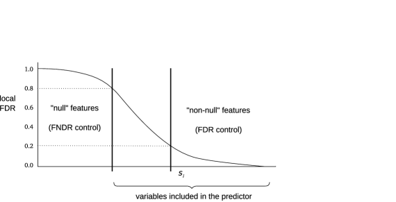
Figure 1: Local false discovery rates as a function of the summary score $S_{i}$. There are three distinct areas: an acceptance and a rejection zone, which are separated by a “buffer zone” in the middle. Note that the features to be included in the classifier by FNDR control of the null genes form a superset of the differentially expressed genes controlled by FDR.

This subtle but important distinction is best illustrated by referring to Figure 1, which plots the local FDR $\mathrm{fdr}(S_{i})=\operatorname{Prob}(\mbox{``null''}|S_{i})$ computed for (and from) the statistic $S_{i}$ of feature $i$. In a list of differentially expressed genes we decide to include, say, genes $i$ with $\mathrm{fdr}(S_{i})<0.2$. A similar constraint on the local false nondiscovery rate, $\mathrm{fndr}(S_{i})<0.2$, gives a confidence set of the null genes. The local false discovery and local false nondiscovery rates add up to one, $\mathrm{fndr}(S_{i})=1-\mathrm{fdr}(S_{i})$. Hence, the set of features to be retained in the classifier have local false discovery rates smaller than 0.8—instead of 0.2. Thus, the features included in the predictor form a superset of the differentially expressed variables. A similar argument applies when using distribution-based Fdr ($q$-values) and Fndr values.

=230pt $\bolds{S_{i}=}$ $\bolds{K}$ arbitrary $\bolds{K=2}$ Correlation present: $\sum_{j=1}^{K}(\tau^{\mathit{adj}}_{i,j})^{2}$ $2(\tau^{\mathit{adj}}_{i})^{2}$ No correlation ($\mathbf{P}=\mathbf{I}$): $\sum_{j=1}^{K}\tau_{i,j}^{2}$ $2\tau_{i}^{2}$

Table 1: The general feature selection score $S_{i}$ and special cases thereof

In short, our proposal is to identify the null features by controlling (local) FNDR, and subsequently using all features except the identified null set in prediction. For estimating FDR quantities, we use the semiparametric approach outlined in Strimmer (2008). Note that this and other FDR procedures assume that there are enough null features so that the null model can be properly estimated [Efron (2004)].

4 Special cases

4.1 Two groups

For $K=2$ the cat score $\bolds{\tau}^{\mathit{adj}}_{k}$ between the group centroid and the pooled mean reduces to the cat score between the two means:

$$\bolds{\tau}^{\mathit{adj}}_{1} = \mathbf{P}^{-1/2}\times\biggl{\{}\biggl{(}\frac{1}{n_{1}}-\frac{1}{n_{1}+n_{2}}\biggr{)}\mathbf{V}\biggr{\}}^{-1/2}\biggl{(}\bolds{\mu}_{1}-\biggl{(}\frac{n_{1}}{n}\bolds{\mu}_{1}+\frac{n_{2}}{n}\bolds{\mu}_{2}\biggr{)}\biggr{)}$$

$$= \mathbf{P}^{-1/2}\times\biggl{\{}\biggl{(}\frac{1}{n_{1}}+\frac{1}{n_{2}}\biggr{)}\mathbf{V}\biggr{\}}^{-1/2}(\bolds{\mu}_{1}-\bolds{\mu}_{2}).$$

Note that $\bolds{\tau}^{\mathit{adj}}_{1}=-\bolds{\tau}^{\mathit{adj}}_{2}$. The feature selection score $S_{i}$ reduces to the squared cat score between the two means; cf. Table 1. Likewise, for $K=2$ the difference $\Delta_{1}^{\mathrm{LDA}}(\mathbf{x})-\Delta_{2}^{\mathrm{LDA}}(\mathbf{x})$ reduces to $\bolds{\omega}^{T}\bolds{\delta}(\mathbf{x})+\log(\frac{\pi_{1}}{\pi_{2}})$ with $\bolds{\omega}=\mathbf{P}^{-1/2}\mathbf{V}^{-1/2}(\bolds{\mu}_{1}-\bolds{\mu}_{2})$ and $\bolds{\delta}(\mathbf{x})=\mathbf{P}^{-1/2}\mathbf{V}^{-1/2}(\mathbf{x}-\frac{\bolds{\mu}_{1}+\bolds{\mu}_{2}}{2})$.

For extensive discussion of the two group case, including comparison of gene rankings with many other test statistics, we refer to Zuber and Strimmer (2009).

4.2 Vanishing correlation

In case of no correlation ($\mathbf{P}=\mathbf{I}$), the cat scores reduce (by construction) to standard $t$-scores between the two centroids of interest, either between the group and the pooled mean (general $K$) or between the two groups ($K=2$). The gene summary $S_{i}$ reduces to the sum of the respective squared $t$-scores (Table 1). The discriminant function reduces to the standard form of diagonal discriminant analysis. The pooled centroids formulation of LDA reduces to that of PAM (except for the shrinkage of the means present in PAM but not in our approach).

5 Remarks

Remark A ((Definition of feature weights)).

The definition of feature weights according to equation (3) is most natural. Other ways of splitting up the product $\bolds{\omega}_{k}^{T}\bolds{\delta}_{k}(\mathbf{x})$ lead to various inconsistencies. For example, instead of using $\bolds{\omega}_{k}=\bolds{\Sigma}^{-1/2}(\bolds{\mu}_{k}-\bolds{\mu}_{\mathrm{pool}})$, it has been suggested to consider $\bolds{\Sigma}^{-1}(\bolds{\mu}_{k}-\bolds{\mu}_{\mathrm{pool}})$, for example, in Witten and Tibshirani (2009), page 627. However, this choice implies that for the case of no correlation variable selection would be based on $\mathbf{V}^{-1}(\bolds{\mu}_{k}-\bolds{\mu}_{\mathrm{pool}})$ rather than on $t$-scores.

Furthermore, dividing the inverse correlation $\mathbf{P}^{-1}$ equally between equations (3) and (4) greatly simplifies interpretation: feature selection takes place on the level of centered, scaled as well as decorrelated predictors $\bolds{\delta}_{k}(\mathbf{x})$. Note that this interpretation is not hampered by the fact that the decorrelation involves all features, because typically there is no substantial correlation between nonnull and null features, so that the overall correlation matrix decomposes into correlation within null and within nonnull variables.

Remark B ((Grouping of features)).

Using cat scores for feature selection also greatly facilitates the grouping of features. Specifically, adding the squared cat scores of each feature contained in a given set (e.g., gene sets specified by biochemical pathways) leads to Hotelling’s $T^{2}$; see Zuber and Strimmer (2009). Note that if another decomposition than that of equation (3) and (4) was used, the connection of cat scores with Hotelling’s $T^{2}$ would be lost.

Remark C ((FDR methods for feature selection)).

The usefulness of false discovery rates for feature selection in prediction is disputed, for example, in Donoho and Jin (2008). What we show here is that the unfavorable performance is due to naive application of FDR, leading to the elimination of too many predictors. If instead FNDR is controlled to determine the null-features to be excluded from the discriminant function, then much more efficient prediction rules are obtained.

Remark D ((Fast computation of matrix square root)).

The inverse square root of the correlation matrix, required in equations (1) and (3.1), can be computed very efficiently for the James–Stein shrinkage estimator; see Zuber and Strimmer (2009) for details.

Remark E ((Normalizing the null model)).

Estimating false discovery rates using summary scores $S_{i}$ (6) assumes as null model a $\chi^{2}$-distribution with unknown parameters. To employ standard FDR software, we apply the cube-root transformation, which provides a normalizing transform for the $\chi^{2}$-distribution [Wilson and Hilferty (1931)].

6 Results

We now illustrate our shrinkage DDA and LDA approaches with variable selection using cat scores and FNDR control by analyzing a number of reference data examples, and compare our results with that of competing approaches. We also investigate the performance of FNDR feature selection in comparison with that of “higher criticism” [Donoho and Jin (2008)].

6.1 Singh et al. (2002) gene expression data

First, we investigated the prostate cancer data set of Singh et al. (2002). This consists of gene expression measurements of $p=6033$ genes for $n=102$ patients, of which 52 are cancer patients and 50 are healthy (thus, $K=2$). To facilitate cross-comparison, we analyzed the data exactly in form as used in Efron (2008a). Our results are summarized in Table 2, and corresponding violin plots [Hintze and Nelson (1998)] are shown in Figure 2.

=220pt Method Prediction Error Features Ebay 0.0920 (0.0000) 000–051 DDA-FDR 0.1682 (0.0093) 000–053 LDA-FDR 0.0989 (0.0056) 000–062 LDA-FNDR 0.0550 (0.0048) 000–131 DDA-FNDR 0.0640 (0.0049) 000–166 PAM 0.0859 (0.0063) 172–482 DDA-ALL 0.3327 (0.0099) 00–6033 []The prediction error of Ebay is taken from Efron (2008a).

Table 2: Prediction errors and number of selected features for Singh et al. (2002) gene expression data. The number in the round brackets is the estimated standard error

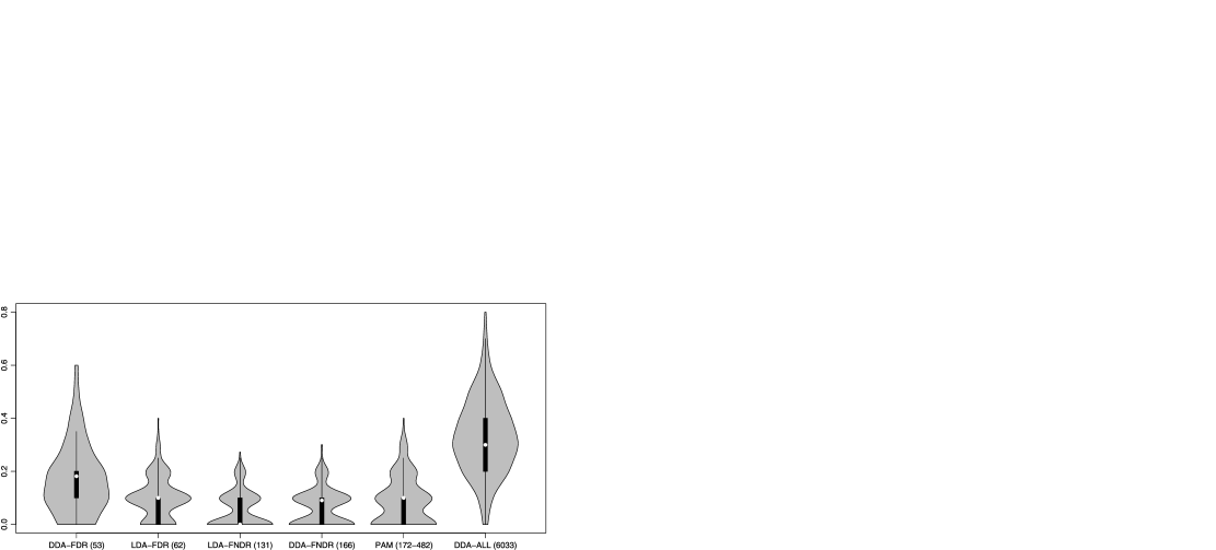
Figure 2: Violin plots of prediction error rates of various classification methods for the Singh et al. (2002) data. The violin plot is a generalization of the box plot, showing the median and upper and lower quartiles, as well as the density. Underlying each plot are 200 estimates of prediction error computed from the 200 splits arising from balanced 10-fold cross-validation with 20 repetitions. The number in round brackets indicates the number of selected features. See also Table 2.

Initially, we assumed zero correlation and applied the shrinkage DDA method. By controlling the local FNDR to be smaller or equal than 0.2, we determined that 5867 genes were null genes, hence, that 166 genes needed to be included in the prediction rule. For comparison, a local FDR cutoff on the same level yielded only 53 genes, lacking the 103 genes in the “buffer zone” between the two cutoffs (cf. Figure 1). Note that we recommend using the larger FNDR-based feature set, not just the 53 genes considered to be differentially expressed.

We estimated the prediction error of the resulting classification rule using balanced 10-fold cross-validation with 20 repetitions. For each of the in total 200 splits we trained a new prediction rule and estimated new feature rankings and FDR statistics, thereby including the selection process in the error estimate to avoid overoptimistic results [Ambroise and McLachlan (2002)]. The number of selected features shown in Table 2 is based on the complete data. However, for estimation of prediction error for each of the splits a new set of features was determined.

For the FNDR-based cutoff with 166 included features, we obtained an estimate of the prediction error of 0.0640, whereas for the naive FDR cutoff resulting in 53 predictors, the error is much higher (0.1682). For comparison, we also computed the error using all 6033 features, yielding a massive 0.3327. The PAM program selected between 172 and 482 genes for inclusion in its predictor with error rate 0.0859 (note that the number of selected features by the PAM algorithm is highly variable and differs from run to run even for the same data set). According to Efron (2008a), the Ebay approach used 51 genes for prediction with error rate 0.092.

If correlation was taken into account, that is, if the order of ranking was determined by cat rather than $t$-scores, interestingly both the number of differentially expressed genes and of the null genes increases, implying that the “buffer zone” shown in Figure 1 becomes smaller. Thus, the LDA classifier with FNDR cutoff contained for this data fewer predictors (131) but at the same time nevertheless achieved the smallest overall prediction error (Figure 2).

6.2 Performance for multiclass reference data sets

=318pt Data Method Prediction error Features DE Lymphoma DDA-FNDR 0.0517 (0.0062) 000–00162 00 ($K=3$, $n=62$, LDA-FNDR 0.0036 (0.0018) 000–00392 55    $p=4026$) PAM 0.0254 (0.0045) 2796–3201 SRBCT DDA-FNDR 0.0007 (0.0007) 0000–0090 62 ($K=4$, $n=63$, LDA-FNDR 0.0000 (0.0000) 0000–0089 76    $p=2308$) PAM 0.0145 (0.0034) 000039–87 Brain DDA-FNDR 0.1892 (0.0146) 000–00033 08 ($K=5$, $n=42$, LDA-FNDR 0.1525 (0.0120) 0000–0102 23    $p=5597$) PAM 0.1939 (0.0112) 0197–5597 []The last column (DE) shows the number of differentially expressed genes, which equals the number of significant features if FDR rather than FNDR is used as criterion.

Table 3: Estimated prediction errors for several multiclass reference data sets

For extended comparison we applied our approach to a number of further reference data sets. In particular, we analyzed gene expression data for lymphoma [Alizadeh et al. (2000)], small round blue cell tumors (SRBCT) [Khan et al. (2001)] and brain cancer [Pomeroy et al. (2002)]. The data sets have in common that all contain more than two classes, thus allowing to study the multi-class summary statistic (6). A summary of the results obtained by shrinkage LDA/DDA and FNDR feature selection and by PAM is given in Table 3.

The Khan et al. (2001) data are very easy to classify. All methods performed equally well on this data, with no substantial difference between the LDA and DDA approaches.

For the lymphoma data set the PAM approach failed to identify a compact set of predictive features. In contrast, the FNDR approach selects a comparatively small number of genes both in the LDA and DDA case. Intriguingly, for this data there were no differentially expressed genes, if correlation is ignored, yet the FNDR criterion yielded 162 nonnull features.

The brain data set is the largest and most difficult data set. Again, the PAM approach failed to determine a stable set of features, whereas FNDR control yielded a compact set of informative predictors. Here, as well as for the lymphoma data, the LDA approach clearly outperformed the DDA approaches in terms of prediction error.

6.3 Comparison with “higher criticism” feature selection

Using the data examples above, we demonstrated that feature selection based on simple FDR cutoffs is not sufficient for prediction. In particular, if features are weak and sparse, it may easily happen that no predictor has sufficiently small false discovery rate to be called significant (cf. the lymphoma data).

=305pt Data Method Prediction error Features local FDR Prostate DDA-HC 0.0707 (0.0055) 129 0.69 LDA-HC 0.0497 (0.0045) 116 0.73 Lymphoma DDA-HC 0.0185 (0.0038) 179 1.00 LDA-HC 0.0000 (0.0000) 345 0.78 SRBCT DDA-HC 0.0035 (0.0016) 138 1.00 LDA-HC 0.0007 (0.0007) 174 1.00 Brain DDA-HC 0.1572 (0.0118) 033 0.77 LDA-HC 0.1417 (0.0108) 131 1.00 []The last column (local FDR) shows the local FDR of the least significant feature.

Table 4: Estimated prediction errors employing higher criticism as feature selection criterion

In such a setting Donoho and Jin (2008) suggest as alternative to FDR-based thresholding the “higher criticism” (HC) approach. The HC criterion is based on $p$-values. For each feature, the $p$-value is centered and standardized using the estimated mean and variance of the corresponding order statistic. The optimal threshold is determined as the maximum of the absolute HC scores within a fraction (say, 10%) of the top ranking features [Donoho and Jin (2008)].

Our feature selection approach based on FNDR control shares with HC that we aim to overcome the limitations resulting from naive application of FDR-based feature selection. For this reason, it is instructive to investigate our shrinkage prediction rule in combination with the HC thresholding procedure. The $p$-values underlying the HC objective function were obtained by fitting a two-component mixture model, so that the same empirical null model was used as in the FDR analysis.

The results are given in Table 4. Again, in all cases the LDA approach using cat scores for feature selection leads to smaller prediction error than employing DDA and $t$-scores. Remarkably, the performance of the FNDR and HC approach are on an equal level, implying that efficient feature selection is indeed possible within the FDR framework. The set of features selected by HC is, on average, a bit smaller than that chosen by FNDR, and larger than the FDR-based set, which indicates that the HC threshold is typically situated in the “buffer zone” of Figure 1.

7 Discussion

7.1 Shrinkage discriminant analysis and feature selection

In this paper we have revisited high-dimensional shrinkage discriminant analysis and presented a very efficient procedure for prediction. Our approach contains three distinct elements:

• the use of James–Stein shrinkage for training the predictor,

• feature ranking based on cat scores, and

• feature selection based on FNDR thresholding.

Employing James–Stein shrinkage estimators is efficient both from a statistical as well as from a computational perspective. Note that shrinkage is used here only as a means to improve the estimated parameters, but not for model selection as in the approaches by Tibshirani et al. (2002) and Guo, Hastie and Tibshirani (2007).

The correlation-adjusted $t$-score (cat score) emerges as a natural gene ranking criterion in the presence of correlation among predictors [Zuber and Strimmer (2009)]. Here we have shown how to employ cat scores in the multi-class LDA setting and demonstrated on high-dimensional data that using cat scores rather than $t$-scores leads to a more effective choice of predictors. We note that the order of ranking induced by the cat and $t$-scores, respectively, may differ substantially. Hence, univariate thresholding procedures to select interesting features will differ, even if the testing procedures account for dependencies.

Finally, we propose feature selection by controlling FNDR rather than FDR and show that this is as efficient in terms of predictive accuracy as when “higher criticism” is employed. Moreover, we explain why variable selection based on FDR leads to inferior prediction rules.

7.2 Recommendations

For extremely high-dimensional data, estimating correlation is very difficult, hence, in this instance we recommend to conduct diagonal discriminant analysis [see also Bickel and Levina (2004)]. From our analysis it is clear the shrinkage DDA as proposed here, combined with variable selection by control of FNDR or HC, is most effective. In contrast to the PAM approach, no randomization procedures are involved and, hence, the prediction rule and the number of selected features are stable.

In all other cases we recommend a full shrinkage LDA analysis, with feature selection based on cat scores. While this approach is computationally more expensive than the shrinkage DDA approach, it has a significant impact on predictive accuracy. Typically, in comparison with DDA, taking account of correlation either leads to more compact feature sets or improved prediction error, or both. Furthermore, relative to competing full LDA approaches, such as Guo, Hastie and Tibshirani (2007), our procedure is computationally fast, due to the avoidance of computer-intensive procedures such as resampling.

Appendix A James–Stein shrinkage estimators for training the LDA predictor

For “small $n$, large $p$” inference of the LDA predictor function (1) and (2) and the cat score (3.1) we rely on three different James–Stein-type estimators.

The correlation matrix is estimated by shrinking empirical correlations $r_{ij}$ toward zero,

$$r_{ij}^{\mathrm{shrink}}=(1-\hat{\lambda}_{1})r_{ij},$$

with estimated intensity

$$\hat{\lambda}_{1}=\min\biggl{(}1,\frac{\sum_{i\neq j}\widehat{\operatorname{Var}}(r_{ij})}{\sum_{i\neq j}r_{ij}^{2}}\biggr{)}$$

[Schäfer and Strimmer (2005)].

The variances are estimated by shrinking the empirical estimates $v_{i}$ toward their median,

$$v_{i}^{\mathrm{shrink}}=\hat{\lambda}_{2}v_{\mathrm{median}}+(1-\hat{\lambda}_{2})v_{i},$$

using

$$\hat{\lambda}_{2}=\min\biggl{(}1,\frac{\sum_{i=1}^{p}\widehat{\operatorname{Var}}(v_{i})}{\sum_{i=1}^{p}(v_{i}-v_{\mathrm{median}})^{2}}\biggr{)}$$

[Opgen-Rhein and Strimmer (2007)].

The class frequencies are estimated following Hausser and Strimmer (2009) by

$$\hat{\pi}_{j}^{\mathrm{shrink}}=\hat{\lambda}_{3}\frac{1}{K}+(1-\hat{\lambda}_{3})\frac{n_{j}}{n},$$

using

$$\hat{\lambda}_{3}=\frac{1-\sum^{K}_{j=1}(n_{j}/n)^{2}}{(n-1)\sum^{K}_{j=1}(1/K-n_{j}/n)^{2}}.$$

Appendix B Relationship to other DDA and LDA approaches

Our proposed shrinkage discriminant approach is closely linked to a number of recently proposed methods.

NSC

The NSC/PAM classification rule was first presented in Tibshirani et al. (2002) and later discussed in more statistical detail in Tibshirani et al. (2003). PAM is a DDA approach, so no gene-wise correlations are taken into account. Genes are ranked according to equation (7), and feature selection is determined by soft-thresholding, using prediction error estimated by cross-validation as optimality criterion.

Ebay

The “Ebay” approach of Efron (2008a) is also a DDA approach. Feature selection is based on an empirical Bayes model that links prediction error with false discovery rates. Thus, it is very similar to PAM but computationally and statistically more efficient. In addition, the “Ebay” algorithm provides correlation corrections of prediction errors; see Section 5 in Efron (2008b).

Clanc and MLDA

The “Clanc” algorithm is described in Dabney and Storey (2007) and the “modified LDA” (MLDA) in Xu, Brock and Parrish (2009). Both methods are based on the LDA framework, and both use James–Stein shrinkage to estimate the pooled covariance matrix. MLDA uses standard $t$-scores for feature selection, whereas Clanc employs a greedy algorithm search to find optimal subsets of features based on a multivariate criterion.

SCRDA

The “shrunken centroids regularized discriminant analysis”(SCRDA) procedure is described in Guo, Hastie and Tibshirani (2007) and uses a similar soft-thresholding procedure for variable selection as PAM. The covariance matrix is estimated by a ridge estimator. Regularization and feature selection parameters are simultaneously determined by cross-validation. The main issues with SCRDA are the computational expense and problems in finding unique parameters [Guo, Hastie and Tibshirani (2007)].

Appendix C Computer implementation

We have implemented the proposed shrinkage discriminant procedures (both DDA and LDA) and the associated FNDR and higher criticism variable selection in the R package “sda,” which is freely available under the terms of the GNU General Public License (version 3 or later) from CRAN (http://cran.r-project.org/web/packages/sda/).

References

- Ackermann and Strimmer (2009) Ackermann, M. and Strimmer, K. (2009). A general modular framework for gene set enrichment. BMC Bioinformatics 10 47.
- Alizadeh et al. (2000) Alizadeh, A. A., Eisen, M. B., Davis, R. E., Ma, C., Lossos, I. S., Rosenwald, A., Boldrick, J. C., Sabet, H., Tran, T., Yu, X., Powell, J. I., Yang, L., Marti, G. E., Moore, T., Hudson, J., Lu, L., Lewis, D. B., Tibshirani, R., Sherlock, G., Chan, W. C., Greiner, T. C., Weisenburger, D. D., Armitage, J. O., Warnke, R., Levy, R., Wilson, W., Grever, M. R., Byrd, J. C., Botstein, D., Brown, P. O. and Staudt, L. M. (2000). Distinct types of diffuse large B-cell lymphoma identified by gene expression profiling. Nature 403 503–511.
- Ambroise and McLachlan (2002) Ambroise, C. and McLachlan, G. J. (2002). Selection bias in gene extraction on the basis of microarray gene-expression data. Proc. Natl. Acad. Sci. USA 99 6562–6566.
- Bickel and Levina (2004) Bickel, P. J. and Levina, E. (2004). Some theory for Fisher’s linear discriminant function, ‘naive Bayes,’ and some alternatives when there are many more variables than observations. Bernoulli 10 989–1010. \MR2108040
- Dabney and Storey (2007) Dabney, A. R. and Storey, J. D. (2007). Optimality driven nearest centroid classification from genomic data. PLoS ONE 2 e1002.
- Donoho and Jin (2008) Donoho, D. and Jin, J. (2008). Higher criticism thresholding: Optimal feature selection when useful features are rare and weak. Proc. Natl. Acad. Sci. USA 105 14790–15795.
- Efron (1975) Efron, B. (1975). The efficiency of logistic regression compared to normal discriminant analysis. J. Amer. Statist. Assoc. 70 892–896. \MR0391403
- Efron (2004) Efron, B. (2004). Large-scale simultaneous hypothesis testing: The choice of a null hypothesis. J. Amer. Statist. Assoc. 99 96–104. \MR2054289
- Efron (2008a) Efron, B. (2008a). Empirical Bayes estimates for large-scale prediction problems. Technical report, Dept. Statistics, Stanford Univ.
- Efron (2008b) Efron, B. (2008b). Microarrays, empirical Bayes, and the two-groups model. Statist. Sci. 23 1–22. \MR2431866
- Fan and Fan (2008) Fan, J. and Fan, Y. (2008). High-dimensional classification using features annealed independence rules. Ann. Statist. 36 2605–2637. \MR2485009
- Friedman (1989) Friedman, J. H. (1989). Regularized discriminant analysis. J. Amer. Statist. Assoc. 84 165–175. \MR0999675
- Guo, Hastie and Tibshirani (2007) Guo, Y., Hastie, T. and Tibshirani, T. (2007). Regularized discriminant analysis and its application in microarrays. Biostatistics 8 86–100.
- Hand (2006) Hand, D. J. (2006). Classifier technology and the illusion of progress. Statist. Sci. 21 1–14. \MR2275965
- Hausser and Strimmer (2009) Hausser, J. and Strimmer, K. (2009). Entropy inference and the James–Stein estimator, with application to nonlinear gene association networks. J. Mach. Learn. Res. 10 1469–1484.
- Hintze and Nelson (1998) Hintze, J. L. and Nelson, R. D. (1998). Violin plots: A box plot-density trace synergism. Amer. Statist. 52 181–184.
- Khan et al. (2001) Khan, J., Wei, J. S., Ringner, M., Saal, L. H., Ladanyi, M., Westermann, F., Berthold, F., Schwab, M., Antonescu, C. R., Peterson, C. and Meltzer, P. S. (2001). Classification and diagnostic prediction of cancers using gene expression profiling and artificial neural networks. Nature Med. 7 673–679.