A bouncing ball model with two nonlinearities: a prototype for Fermi acceleration

Abstract

Some dynamical properties of a bouncing ball model under the presence of an external force modeled by two nonlinear terms are studied. The description of the model is made by use of a two dimensional nonlinear measure preserving map on the variables velocity of the particle and time. We show that raising the straight of a control parameter which controls one of the nonlinearities, the positive Lyapunov exponent decreases in the average and suffers abrupt changes. We also show that for a specific range of control parameters, the model exhibits the phenomenon of Fermi acceleration. The explanation of both behaviours is given in terms of the shape of the external force and due to a discontinuity of the moving wall’s velocity.

1 Introduction

The bouncing ball model consists of a classical particle of mass $m$ which is confined to bounce between two infinitely heavy and rigid walls [1]. One of the walls is assumed to be fixed while the other one moves in time according to a periodic function. This model, also known as the Fermi-Ulam model (FUM), is a simple dynamical system that can be modeled using the formalism of discrete mappings. Moreover, many tools developed to characterise such a model show to have great applicability in more complex mappings. Considering the FUM, many results are known in the literature. Particularly for the particle suffering elastic collisions with either walls, it is known that the phase space of the model is of mixed kind [2] in the sense that depending on the combination of both the control parameters and initial conditions, invariant spanning curves limiting the size of chaotic seas and Kolmogorov-Arnold-Moser (KAM) islands can all be observed. The presence of the invariant spanning curves yields in a limit for the energy gain of a bouncing particle, thus the Fermi acceleration (unlimited energy gain of the particle) is not observed. A similar version of the model, called as bouncer [3], consists of a classical particle, in the presence of a constant gravitational field, suffering elastic collisions with a periodically moving platform. The returning mechanism of the bouncer model, a mechanism that injects the particle for a next collision with the moving wall, is rather distinct of the FUM. In the bouncer, it is due only to the gravitational field while in the FUM it is given by a collision with a fixed wall. These differences yield in a profound consequence for the dynamics of a bouncing particle. Depending on the control parameter, the unlimited energy gain is observed in the bouncer model, a phenomenon that is not present in FUM with periodic and smooth oscillations. The differences were clarified by Lichtenberg, Lieberman and Cohen [4]. Hybrid versions of the FUM and bouncer were recently studied [5, 6] as well as a stochastic version of the FUM [7].

There are also many important results concerning the inclusion of damping forces on both the models (see for example Ref. [8] for a short review). One of them is the presence of a drag force [9], so that the particle is moving inside a gas with the dissipation acting on the particle along its trajectory. The dynamics of the problem is, generally, given by a nonlinear mapping that is obtained via the solution of Newton’s law. A different kind of dissipation can be introduced via inelastic hits of the particle with the walls. Thus, there is a restitution coefficient that makes the particle experiences a fractional loss of energy upon collisions. Despite both kinds of damping often occur in nature, they have profound and different consequences in the dynamics of the models. As an example, in Refs. [10, 11] and considering inelastic collisions, Tsang and Lieberman considered the simplified FUM (both the walls are fixed but the particle changes energy and momentum upon collisions with one of the wall as if the wall were moving) with inelastic impacts. They have evidenced contraction on the phase space and in particular, observed the presence of a strange attractor. Recently, a rather similar version of the dissipative model [12], confirmed the property of area contraction and in addition, a boundary crisis was characterised. Additionally, a family of boundary crisis was observed when collisions with the two walls are inelastic [13]. The bouncer model was also considered under inelastic collisions. For example, in [14] Holmes discusses the appearances of horseshoes in the inelastic bouncer and gave an illustration of a homoclinic orbit in such a model. After that, Everson [15] presents and discusses with many numerical simulations the appearance of period doubling cascade in the damping bouncer model. Period doubling cascade was also observed in [16] for the completely inelastic collisions. The presence of frictional force however was considered by Luna-Acosta [17] and Naylor, Sanchéz and Swift [18] in the bouncer model. They too observed period doubling cascades and in special Luna-Acosta [17] has achieved analytically dimensional reduction for the limit of high dissipation.

In this letter, we study a non dissipative version of a bouncing ball model seeking to understand and describe some of its dynamical properties considering however that the motion of the moving wall is given via a crank-connecting rod scheme. For such a scheme, it is known that there are two nonlinearities present in the model and each of them play important rules in the dynamics. Depending on certain ranges of control parameters, there can be profound consequences on the dynamics of the system. Particularly, when one of the two control parameters is raised, the positive Lyapunov exponent experiences a drastic reduction. It is also important to say that the particle is in the total absence of any external field. Other important result for this model is that it yields, for specific control parameter values, the phenomenon of Fermi acceleration (unlimited energy growth). The phenomenon is characterised, for the first time in the present model, in terms of a discontinuity of the derivative of the wall’s position with respect to the time, thus leading the particle to acquire unlimited energy gain.

This paper is organised as follows. In section 2 we present the model and the expressions of the mapping that fully describes the dynamics of the system. Section 2 is also devoted to a discussion of the numerical results and the behaviour of the positive Lyapunov exponent. In section 3 we propose a simplified version of the model and study the behaviour of the average velocity as function of a control parameter. We show that Fermi acceleration emerges naturally from the deterministic dynamics of the model for specific control parameter values. Final remarks and conclusions are drawn in section 4.

2 The model and the mapping

The model is described using a two dimensional mapping for the variables $(v_{n},t_{n})$, where $v_{n}$ and $t_{n}$ are the corresponding velocity of the particle and time immediately after the n^th collision with the moving wall. We assume that one wall is fixed at $x=l$ and that the motion of the moving wall is given by $s(t)=R\cos(wt)+\sqrt{L^{2}-R^{2}\sin^{2}(wt)}$ (we stress the term $wt$ in the equation of $s(t)$ is represented by the variable $\phi$ in Fig. 1), where $R$ denotes the radii of the crank, $L$ is the length of the connecting rod and $w$ is the corresponding frequency of oscillation. Figure 1 illustrates the model under consideration. We stress the equation for $s(t)$ is easily obtained from the condition of $R\sin(\phi)=L\sin(\psi)$, as can be seen in Fig. 1.

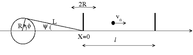
Figure 1: Illustration of the model under consideration.

Before we write the equations of the mapping, let us first discuss the initial conditions. We assume that, at a time $t=t_{n}$, the particle is at the position $x_{p}(t_{n})=s(t_{n})$ with velocity $v=v_{n}>0$. Thus such an initial condition can be considered as if the dynamics were already running in the system along the time. We emphasise that two different kinds of collisions can be observed namely: (i) multiple hits with the moving wall and (ii) a single hit with the moving wall. In case (i), the particle suffers a collision with the moving wall but then, before it leaves the collision zone, which is defined as $x\in[-R,R]$, the particle experiences a second and then successive impact with the moving wall. Such kind of collisions becomes rare in the limit of high energy but they are quite often to be observed in the regime of low energy. It is also easy to see that there are too many control parameters in the model, 4 in total, namely $R$, $L$, $l$ and $w$ and that the dynamics of the system does not depend on all of them. It is convenient to define dimensionless and more appropriated variables. We define $\epsilon=R/l$, $r=R/L$, $V_{n}=v_{n}/(wl)$ and measure the time in terms of the number of oscillations of the moving wall $\phi_{n}=wt_{n}$. For the dimensionless variables, we consider that the range for $\epsilon$ is $\epsilon\in[0,1]$ and for $r$ is $r\in[0,1]$. The limit of $r\rightarrow 0$ corresponds to $L\rightarrow\infty$ and $r\rightarrow 1$ is obtained for $L\rightarrow R^{+}$. With this new set of variables, the mapping that describes the dynamics of the system is written as

$$T:\left\{\begin{array}[]{ll}\phi_{n+1}=[\phi_{n}+\Delta T_{n}]~{}~{}{\rm mod(2\pi)}\\ V_{n+1}=V_{n}^{*}-2\epsilon\sin(\phi_{n+1})\left[1+{{r\cos(\phi_{n+1})}\over{\sqrt{1-r^{2}\sin^{2}(\phi_{n+1})}}}\right]\\ \end{array}\right.,$$ (1)

where the expressions of $V_{n}^{*}$ and $\Delta T_{n}$ depend on the kind of collision. For case (i), which corresponds to the multiple hits with the moving wall, the corresponding expressions are $V_{n}^{*}=-V_{n}$ and $\Delta T_{n}=\phi_{c}$ with $\phi_{c}$ obtained by the solution of $G(\phi_{c})=0$ with $G(\phi_{c})$ given by

$$G(\phi_{c}) = \epsilon\cos(\phi_{n}+\phi_{c})-\epsilon\cos(\phi_{n})-V_{n}\phi_{c}+{{\epsilon}\over{r}}\sqrt{1-r^{2}\sin^{2}(\phi_{n}+\phi_{c})}-$$

$$- {{\epsilon}\over{r}}\sqrt{1-r^{2}\sin^{2}(\phi_{n})}~{}.$$

A solution of the function $G(\phi_{c})$ for $\phi_{c}\in(0,2\pi]$ corresponds to a collision of the particle with the moving wall and it is obtained numerically.

Let us now consider the case where the particle leaves the collision zone, i.e. case (ii). The corresponding expressions are $V_{n}^{*}=V_{n}$, $\Delta T_{n}=\phi_{T}+\phi_{c}$ where $\phi_{T}$ corresponds to the elapsed time the particle spends travelling from the last hit with the moving wall, up to suffering an elastic reflection with the static wall and be reflected backwards, therefore until the entrance of the moving wall. Thus, $\phi_{T}$ is given by

$$\phi_{T}={{2+\left({{\epsilon}\over{r}}-{{\epsilon}\over{r}}\sqrt{1-r^{2}\sin^{2}(\phi_{n})}\right)-\epsilon\cos(\phi_{n})-\epsilon}\over{V_{n}}}~{}.$$ (3)

The term $\phi_{c}$ is numerically obtained from $F(\phi_{c})=0$ for $\phi_{c}\in[0,2\pi)$ where the function $F(\phi_{c})$ is given by

$$F(\phi_{c})=\epsilon\cos(\phi_{n}+\phi_{T}+\phi_{c})+{{\epsilon}\over{r}}\sqrt{1-r^{2}\sin^{2}(\phi_{n}+\phi_{T}+\phi_{c})}-{{\epsilon}\over{r}}-\epsilon+V_{n}\phi_{c}~{}.$$ (4)

After some straightforward algebra, it is easy to show that the mapping (1) preserves the following phase space measure

$$d\mu=\left[V+\epsilon\sin(\phi)\left(1+{{r\cos(\phi)}\over{\sqrt{1-r^{2}\sin^{2}(\phi)}}}\right)\right]dVd\phi~{}.$$ (5)

We stress that in the limit of $r\rightarrow 0$, the results for the one-dimensional Fermi accelerator model are all recovered [5, 19].

Figure 2 shows

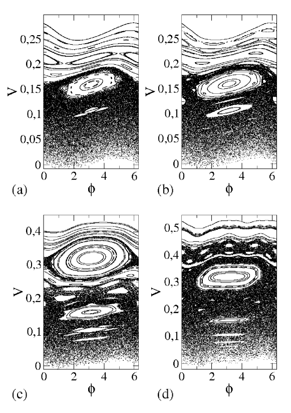
Figure 2: Phase space generated from mapping (1) and control parameter $\epsilon=0.01$ and: (a) $r=0.1$, (b) $r=0.3$, (c) $r=0.6$ and (d) $r=0.9$.

the corresponding phase space obtained via iteration of mapping (1) for the control parameter $\epsilon=0.01$ and: (a) $r=0.1$, (b) $r=0.3$, (c) $r=0.6$ and (d) $r=0.9$. We can clearly see that the shape of the phase space changes as the control parameter $r$ varies. On the other hand, the mixed form is preserved in the sense that a large chaotic sea, which surrounds KAM islands, is limited by a set of invariant spanning curves. One can also note that the position of the lowest invariant spanning curve raises as the control parameter $r$ increases. In our simulations we will consider values for $r$ that may approaches the unity, moreover in the range of $r\in[0,1]$. However for a real experimental system, in which damping forces can not be neglected, such values for $r$ have no much interest. This is mainly because the damping force can acquires larger values as compared to the component of the force with respect to the motion (for instance, it happens for large values of the angle $\psi$) and therefore, lead the system to reach the rest.

The two natural questions that we are interested in concern on the properties of the chaotic sea (see Fig. 2), like the positive Lyapunov exponent and the average velocity of the particle. Our main goal is to describe their behaviour as function of the control parameter $r$. We think this study is of interest because the control parameter $r$ directly controls the straight of a nonlinearity of the model. For small values of $r$, results of the FUM should be obtained. Moreover, we expect that the results obtained for $r\rightarrow 1$ contribute towards a better understanding of this model for such a range of $r$ and, in particular as we will see in Sec. 3, in a description of the phenomenon of Fermi acceleration. The behaviour of the Lyapunov exponent is described in this section while the average velocity is discussed in section 3.

We concentrate to investigate the behaviour of the positive Lyapunov exponent for the chaotic sea. It is well known that the Lyapunov exponent is commonly used as a tool to characterise sensitivity to initial conditions. Figure 3

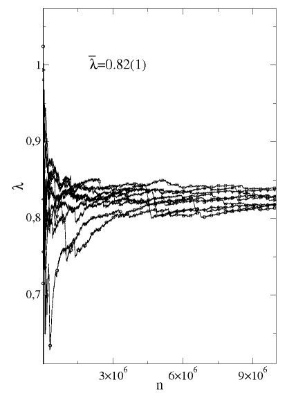
Figure 3: Positive Lyapunov exponent for 10 different initial conditions randomly chosen along the chaotic sea in the low energy regime. The control parameters used were $\epsilon=0.01$ and $r=0.1$.

shows the asymptotic convergence of the positive Lyapunov exponent for the control parameters $\epsilon=0.01$ and $r=0.1$. The ensemble average of $10$ different initial conditions randomly chosen along the chaotic sea gives $\bar{\lambda}=0.82\pm 0.01$, where the error $0.01$ denotes the standard deviation of the ten samples. Each initial condition was iterated up to $10^{7}$ collisions with the moving wall. The method used to obtain the Lyapunov exponents is described in the Appendix.

Let us discuss the behaviour of the positive Lyapunov exponent as function of $r$. Figure 4 shows

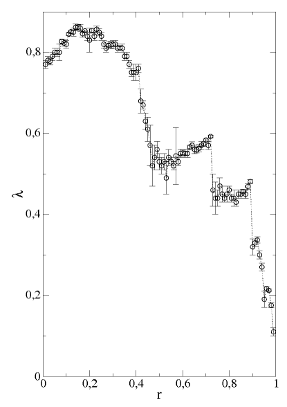
Figure 4: Positive Lyapunov exponent as function of $r$ for a fixed $\epsilon=0.01$.

the behaviour of $\lambda\times r$. We can see that, in the limit of $r\rightarrow 0$, the positive Lyapunov exponent recovers the value of the one-dimensional Fermi accelerator model [5, 19]. The positive Lyapunov exponent then grows slightly, having a maximum value around $r=0.15$ and then decreases almost monotonically until around $r=0.5$. Then it starts grow again until $r\approx 0.7$ when it suddenly decreases. Other abrupt change is observed for $r\approx 0.89$. Thus, the two main questions that arise from Fig. 4 are: (i) why does the positive Lyapunov exponent decreases in the average, instead of growth, as $r$ raises? (ii) what is the explanation of the abrupt changes in $\lambda$?

The answer for question (i) comes from the shape of the function that describes the motion of the moving wall. Figure 5 shows

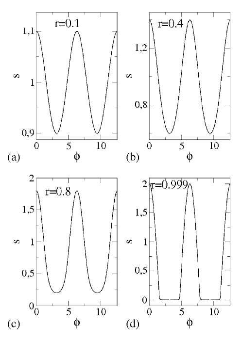
Figure 5: Plot of $S(\phi)$ for two periods in $\phi$ considering the control parameters $\epsilon=0.01$ and: (a) $r=0.1$, (b) $r=0.4$, (c) $r=0.8$ and (d) $r=0.999$.

four different plots of $S(\phi)=r\cos(\phi)+\sqrt{1-r^{2}\sin^{2}(\phi)}$ (for sake of clarity, we show two periods in $\phi$ for $S(\phi)$), which describes the motion of the moving wall for four different values of $r$ namely: (a) $r=0.1$, (b) $r=0.4$, (c) $r=0.8$ and (d) $r=0.999$. For $r=0.1$, the function looks like a cosine function but as $r$ increases, the shape changes substantially. It thus become to have two regimes of variation where one of them is characterised by a constant plateau in the limit of $r\rightarrow 1$, as can be seen in the range of $\phi\in(\pi/2,3\pi/2)$ and a regime of fast variation, which is given by the complementary values of $\phi$. In the limit case of $r=1$, the function $S(\phi)$ has indeed discontinuities in its derivative for two values of $\phi$, namely $\phi=\pi/2$ and $\phi=3\pi/2$. As we will see in the next section, the discontinuities for $S(\phi)$ yield a profound consequence in the dynamics of the system thus leading the particle to exhibit unlimited energy growth. The large plateaus imply that the particle, when suffers collisions with the moving wall does not change substantially its velocity value since such plateaus lead in an “almost” null velocity for the moving wall. Thus the time that the particle spends until a next hit with the moving wall is almost the same as it spent in the previous collisions. It then implies that the particle, in a chaotic orbit, can experience many more collisions with the moving wall without substantially changing its energy as it would experiences if the plateaus were absent. Then, the form of $S(\phi)$ for large values of $r$ yields in reducing the chaoticity of the system in the average.

We will now discuss a possible answer for question (ii), i.e., the explanation of the sudden changes in $\lambda$. They are basically related to the destruction of the lowest energy invariant spanning curve together with a destruction of small chaotic layers. Considering the case of low energy and for $r=0.69$, the system has a large chaotic sea (the black region of Fig. 6(c)) which shares boundary with a thin chaotic layer (the red region of Fig. 6(c)), as can be seen in Fig. 6.

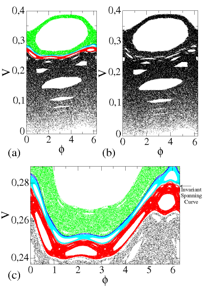
Figure 6: (a) Illustration of chaotic behaviour generated by $5$ different initial conditions for the control parameters $\epsilon=0.01$ and $r=0.69$. (b) Iteration of a single initial condition, evidencing the chaotic behaviour, for $\epsilon=0.01$ and $r=0.72$. (c) Zoom in of part (a) where it is easy to see an invariant spanning curve and chaotic layers.

Above this chaotic layer, there is an invariant spanning curve (brown curve of Fig. 6(c)). Above yet of such curve we can see two thin chaotic layers (light blue and dark blue) and a relatively large chaotic sea (green region) surrounding a KAM island (see for instance Fig. 2(c)). Each of these chaotic regions were characterised in terms of Lyapunov exponents. Their corresponding values were: for the black region we obtained $\lambda_{\rm b}=0.574(6)$; for the red region $\lambda_{\rm r}=0.072(1)$; for the light blue $\lambda_{\rm lb}=0.0110(4)$; for the dark blue $\lambda_{\rm db}=0.0152(2)$ and for the green region $\lambda_{\rm g}=0.218(1)$. For $r=0.72$, which is quite close to $r=0.69$, those regions shown in Fig. 6(a) were all merged into a single and large chaotic sea characterised by a positive Lyapunov exponent $\lambda=0.46(5)$. The merged regions are shown in Fig. 6(b). After the destruction of the thin structures shown in Fig. 6(a), the chaotic sea in the low energy region can spreads over a larger accessible region of the phase space. So we can consider that, after the transition, the positive Lyapunov exponent could be obtained by an average of the previous values for the corresponding chaotic regions therefore taking into account the fraction of area occupied individually by each region. To check whether this supposition is correct, we have obtained the fraction of each chaotic region previous to the control parameter variation i.e. for $r=0.69$. We have defined a grid of $84$ initial conditions for the $\phi$-axis, limited to the interval $\phi\in[0,2\pi)$, and $127$ for the $V$-axis considering the interval $V\in[0,0.38813]$. The value $0.38813$ corresponds to the higher value of the velocity obtained for the chaotic sea shown in the green region of Fig. 6(c). Thus in the total, we considered $10668$ different initial conditions. Each of them were evolved in time for $n=10^{7}$ collisions with the moving wall and their Lyapunov exponents evaluated. The obtained value was compared to the Lyapunov exponent of the chaotic regions so that we were able to compare the corresponding fraction of initial conditions which belongs to one region or to another one. Applying this procedure for all the chaotic regions shown in Fig. 6(c), we found that the black chaotic sea fills a fraction of $P_{\rm b}=0.8261$ of the entire chaotic region. The red region corresponds to $P_{\rm r}=0.0279$, when the light blue has a fraction of $P_{\rm lb}=0.0103$, the dark blue is $P_{\rm db}=0.0038$ and finally the green region corresponds to a fraction of $P_{\rm g}=0.1319$. After the transition, we could assume that the positive Lyapunov exponent is obtained by

$${\bar{\lambda}}=\lambda_{\rm b}P_{\rm b}+\lambda_{\rm r}P_{\rm r}+\lambda_{\rm lb}P_{\rm lb}+\lambda_{\rm db}P_{\rm db}+\lambda_{\rm g}P_{\rm g}~{}.$$ (6)

Evaluating Eq. (6) we found ${\bar{\lambda}}=0.50$ which is a rather acceptable value as compared to the value obtained via numerical simulation of the chaotic sea after the destruction $\lambda=0.46(5)$.

The abrupt change in $\lambda$ around the value of $r\approx 0.89$ is explained by using the same arguments. We stress that similar results were observed in a rather distinct model [20].

3 A simplified version of the model and Fermi acceleration

Other important conclusion that arises from the shape of the function $S(\phi)$ is related to the energy gain of the bouncing particle. As $r$ approaches the unity, the variation of the moving wall position becomes more fast for specific ranges of $\phi$. It implies that the particle can acquires, for specific ranges of $\phi$, large values of velocity upon collisions with the moving wall for those regions of fast variation of $S(\phi)$. Such a result can be seen in Fig. 2 by the position of the lowest energy invariant spanning curve which assume higher values as the control parameter $r$ raises. To illustrate such an argument more clearly, it is important to look at the behaviour of the average velocity for sufficiently long time. To do this, we will make use of a simplification in the mapping (1) with the main goal of speeding up our numerical simulations and avoid solving the equations $G(\phi_{c})=0$ and $F(\phi_{c})=0$. This simplification, which is commonly used in the literature (see Refs. [1, 5, 7, 21, 22, 23]), consists in assume that both walls are fixed. However, when the particle hits one of them, it exchanges energy and momentum as if the wall were moving. This procedure retains the nonlinearity of the problem and yields a huge advantage of avoid solving transcendental equations. The mapping is then given by

$$T:\left\{\begin{array}[]{ll}\phi_{n+1}=[\phi_{n}+{{2}\over{V_{n}}}]~{}~{}{\rm mod(2\pi)}\\ V_{n+1}=\left|V_{n}-2\epsilon\sin(\phi_{n+1})\left[1+{{r\cos(\phi_{n+1})}\over{\sqrt{1-r^{2}\sin^{2}(\phi_{n+1})}}}\right]\right|\\ \end{array}\right..$$ (7)

Although this simplification brings the advantage of allowing very fast simulations as compared to those of the complete version, it also gives rise to a problem that we need to avoid. In the complete model, depending on the combination of both velocity and phase of the moving wall, it is possible for the particle, after suffering a collision with the time varying wall, to suffer a second successive collision before exiting the collision area, as well as possibly having a negative velocity following the first such a collision. In the simplified model, non-positive velocities are forbidden because they are equivalent to the particle travelling beyond the wall. In order to avoid such problems, if after the collision the particle has a negative velocity, we inject it back with the same modulus of velocity. Such a procedure is effected perfectly by the use of a modulus function. Note that the velocity of the particle is reversed by the modulus function only if, after the collision, the particle remains travelling in the negative direction. The modulus function has no effect on the motion of the particle if it moves in the positive direction after the collision. We stress that this approximation is valid only for small values of $\epsilon$.

We now discuss the procedure used to obtain the average velocity of the particle. Firstly we obtain the average velocity proceeding with an average over the orbit, i.e.

$$V_{i}={{1}\over{n}}\sum_{j=1}^{n}V_{i,j}~{},$$ (8)

where $j$ denotes the number of collisions. The second average is made in an ensemble of $M=10^{3}$ different initial conditions so that the average value is defined as

$${\bar{V}}={{1}\over{M}}\sum_{i=1}^{M}V_{i}~{},$$ (9)

with $i$ corresponding to a sample in an ensemble of $M$ different initial conditions.

Figure 7(a) shows

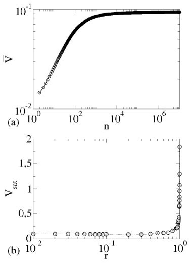
Figure 7: (a) Behaviour of ${\bar{V}}\times n$ for the control parameters $r=0.01$ and $\epsilon=0.01$. (b) Plot of $V_{\rm sat}\times r$ for a fixed $\epsilon=0.01$.

the behaviour of ${\bar{V}}\times n$ for the control parameters $\epsilon=0.01$ and $r=0.01$ considering $n=10^{7}$ iterations. We can see that the velocity of the particle grows for short iterations and then suddenly it bends towards a regime of saturation for sufficiently long time. Moreover, we are interested in the behaviour of the asymptotic values of ${\bar{V}}$. Figure 7(b) shows the behaviour of ${\bar{V}}$ for long iterations, which we will referr to it as $V_{\rm sat}$. The behaviour of $V_{\rm sat}$ can be described for two different ranges of $r$. The first range is for $r<0.9$ where we can see that $V_{\rm sat}$ is almost constant for the region of $r\in[0,0.9)$. The second range of $r$ is considered for $r\geq 0.9$. It is important to say that, when $r=1$ the expression of the “moving wall” velocity presents discontinuities for $\phi=\pi/2$ and $\phi=3\pi/2$. Thus, it is convenient to define a new parameter $\mu=1-r$ and then study the behaviour of $V_{\rm sat}$ as a function of $\mu$. This new control parameter has a practical application because it brings the criticality of the model to $\mu=0$. Figure 8 shows

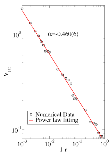
Figure 8: Plot of $V_{\rm sat}\times\mu$ for a fixed $\epsilon=0.01$. A power law fitting gives that $\alpha=-0.460(6)\cong-0.5$.

the behaviour of $V_{\rm sat}\times\mu$ for a fixed control parameter $\epsilon=0.01$. We can describe such a behaviour according to

$$V_{\rm sat}\propto\mu^{\alpha}~{}.$$ (10)

After fitting a power law in Fig. 8, we obtain $\alpha=-0.460(6)\cong-0.5$. This kind of behaviour for $V_{\rm sat}$ confirms that, in the limit of $r\rightarrow 1$, the present model shows the phenomenon of Fermi acceleration. This result has a clear explanation in terms of the KAM theorem. As it was discussed by Lichtenberg, Lieberman and Cohen [4], if the expression of the periodic wall’s velocity has a sufficient number of continuous derivatives, then it is possible to obtain invariant spanning curves separating different portions of the phase space. Particularly they are useful to prevent unlimited energy growth for a bouncing particle. Moreover, it was estimated by Moser [24] that three continuous derivatives for the moving wall velocity is a sufficient condition for the existence of KAM surfaces (by instance, invariant spanning curves). However, in the present model and considering the limit of $r\rightarrow 1$, the expression of the velocity shows discontinuities for $\phi=\pi/2$ and $\phi=3\pi/2$, so that the invariant spanning curves are not observed for $r=1$ and consequently, Fermi acceleration is present.

4 Conclusions

In summary, we have studied a non dissipative version of a classical bouncing ball model under the presence of two nonlinearities. Our results show that, as one of the two control parameters varies, the positive Lyapunov exponent diminish in the average and experiences sudden changes. We have explained such a behaviour by the shape of the moving wall and due to the destruction of invariant spanning curves and thin chaotic layers. We have also shown that in the limit of $r\rightarrow 1$, the present model exhibits unlimited energy growth. This phenomenon was explained by using a discontinuity of the moving wall’s velocity.

Appendix

In this section, we briefly discuss the procedure used to obtain the Lyapunov exponents. In effect, the procedure consists in evolving the system over a long time from two slightly different initial conditions. If the two trajectories diverge exponentially in time the orbit is called chaotic, and the Lyapunov exponent obtained is positive. If the Lyapunov exponent is negative, the orbit may be either periodic or quasi-periodic. Let us now describe the procedure used to obtain the Lyapunov exponents numerically. They are defined as [25]

$$\lambda_{j}=\lim_{n\rightarrow\infty}\ln{|\Lambda_{j}|},~{}~{}~{}~{}~{}~{}~{}j=1,2,$$

where $\Lambda_{j}$ are the eigenvalues of $M=\prod_{k=1}^{n}J_{k}(V_{k},\phi_{k})$ and $J_{k}$ is the Jacobian matrix evaluated over the orbit $(V_{k},\phi_{k})$. The Jacobian matrix is defined as

$$J=\left(\begin{array}[]{ll}{{\partial V_{n+1}}\over{\partial V_{n}}}&{{\partial V_{n+1}}\over{\partial\phi_{n}}}\\ {{\partial\phi_{n+1}}\over{\partial V_{n}}}&{{\partial\phi_{n+1}}\over{\partial\phi_{n}}}\\ \end{array}\right).$$

In order to evaluate the eigenvalues of $M$, we use the fact that $J$ can be written as a product of $J=\Theta T$, where $\Theta$ is an orthogonal matrix and $T$ is a right upper triangular one. We now define the elements of these matrices as

$$\Theta=\left(\begin{array}[]{ll}\cos(\theta)&-\sin(\theta)\\ \sin(\theta)&~{}~{}\cos(\theta)\\ \end{array}\right),~{}~{}T=\left(\begin{array}[]{ll}T_{11}&T_{12}\\ 0&T_{22}\\ \end{array}\right).$$

Since $M$ is defined as $M=J_{n}J_{n-1}\ldots J_{2}J_{1}$, we can introduce the identity operator, rewrite $M$ as $M=J_{n}J_{n-1}\ldots J_{2}\Theta_{1}\Theta_{1}^{-1}J_{1}$, and define $\Theta_{1}^{-1}J_{1}=T_{1}$. The product $J_{2}\Theta_{1}$ defines a new matrix $J_{2}^{*}$. In a following step, we may write $M$ as $M=J_{n}J_{n-1}\ldots J_{3}\Theta_{2}\Theta_{2}^{-1}J_{2}^{*}T_{1}$. The same procedure yields $T_{2}=\Theta_{2}^{-1}J_{2}^{*}$. The problem is thus reduced to the evaluation of the diagonal elements of $T_{i}:T_{11}^{i},T_{22}^{i}$. Using the $\Theta$ and $T$ matrices, we find the eigenvalues of $M$, given by

$$T_{11}={{j_{11}^{2}+j_{21}^{2}}\over{\sqrt{j_{11}^{2}+j_{21}^{2}}}},~{}~{}T_{22}={{j_{11}j_{22}-j_{12}j_{21}}\over{\sqrt{j_{11}^{2}+j_{21}^{2}}}}.$$

We can then evaluate the Lyapunov exponent using the relation

$$\lambda_{j}=\lim_{n\rightarrow\infty}\sum_{k=1}^{n}{1\over{n}}\ln{|T^{k}_{jj}|},~{}~{}~{}~{}~{}~{}~{}j=1,2.$$

It is interesting to observe that $\lambda_{1}=-\lambda_{2}$, because the map is measure-preserving.

References

References

- [1] Lichtenberg A J, Lieberman M A 1992 Regular and Chaotic Dynamics, Applied Mathematical Sciences vol 38 (New York: Springer-Verlag)
- [2] Lieberman M A, Lichtenberg A J 1972 Phys. Rev. A 5 1852
- [3] Pustylnikov L D, 1977 Trudy Moskov. Mat. Obsc. 34 1
- [4] Lichtenberg A J, Lieberman M A, Cohen R H 1980 Physica D 1 291
- [5] Leonel E D, McClintock P V E 2005 J. Phys. A: Math. Gen. 38 823
- [6] Ladeira D G, Leonel E D 2007 Chaos 17 023229
- [7] Karlis A K, Papachristou P K, Diakonos F K, Constantoudis V, Schmelcher P 2006 Phys. Rev. Lett. 97 194102; 2007 Phys. Rev. E 76 016214
- [8] Leonel E D, McClintock P V E 2006 J. Phys. A: Math. Gen. 39 11399
- [9] Leonel E D, McClintock P V E 2006 Phys. Rev. E 73 066223
- [10] Tsang K Y, Lieberman M A 1986 Physica D 21 401
- [11] Lieberman M A, Tsang K Y 1985 Phys. Rev. Lett. 5 908
- [12] Leonel E D, McClintock P V E 2005 J. Phys. A: Math. Gen. 38 L425
- [13] Leonel E D, Egydio de Carvalho R 2007 Phys. Lett. A 364 475
- [14] Holmes P J 1982 J. Sound and Vibr. 84 173
- [15] Everson R M 1986 Physica D 19 355
- [16] Luck J M, Mehta A 1993 Phys. Rev. E 48 3988
- [17] Luna-Acosta G A 1990 Phys. Rev. A 42 7155
- [18] Naylor M A, Sánchez P, Swift M R 2002 Phys. Rev. E 66 57201
- [19] Leonel E D, da Silva J K L, Kamphorst S O 2004 Physica A 331 435
- [20] Leonel E D, da Silva J K L 2003 Physica A 323 181
- [21] Leonel E D, McClintock P V E, da Silva J K L 2004 Phys. Rev. Lett. 93 014101
- [22] Ladeira D G, da Silva J K L 2006 Phys. Rev. E 73 026201
- [23] da Silva J K L, Ladeira D G, Leonel E D, McClintock P V E, Kamphorst S O 2006 Braz. J. Phys 36 700
- [24] Moser J 1973 Stable and Random Motions in Dynamical Systems, Ann. of Math. vol 77 (Princeton: Princeton Univ. Press.)
- [25] Eckmann J P, Ruelle D 1985 Rev. Mod. Phys. 57 617