Abstract

We present a detailed review of scaling behavior in the magnetically underdoped cuprate superconductors (hole dopings less than $0.20$) and show that it reflects the presence of two coupled components throughout this doping regime: a non-Landau Fermi liquid and a spin liquid whose behavior maps onto the theoretical Monte Carlo calculations of the 2D Heisenberg model of localized Cu spins for most of its temperature domain. We use this mapping to extract the doping dependence of the strength, $f(x)$ of the spin liquid component and the effective interaction, $J_{eff}(x)$ between the remnant localized spins that compose it; we find both decrease linearly with x as the doping level increases. We discuss the physical origin of pseudogap behavior and conclude that it is consistent with scenarios in which the both the large energy gaps found in the normal state and their subsequent superconductivity are brought about by the coupling between the Fermi liquid quasiparticles and the spin liquid excitations, and that differences in this coupling between the 1-2-3 and 2-1-4 materials can explain the measured differences in their superconducting transition temperatures and other properties.

1 Introduction

Explaining the anomalous normal state properties of the so-called pseudogap regime of the underdoped cuprate superconductors is widely regarded as an essential step toward understanding the basic physics of these materials and unlocking the mechanism of their superconductivity[1]. Perhaps the most striking aspect of these is the universal, or scaling, behavior, first identified in measurements of their temperature-dependent uniform magnetic susceptibility[2], and since found in Knight shift, transport, and entropy measurements. In the present article we present a detailed review of scaling behavior in the underdoped cuprates that extends previous analyses of its manifestations in both static and low frequency dynamic behavior as well as that seen in inelastic neutron scattering (INS) experiments. Our review updates our earlier analysis[3] and the results presented in Norman et al.[1], and complements the recent review of gap behavior presented in Hüfner et al.[4].

We find that from zero hole doping until planar doping levels of $\sim 0.2$ are reached, the scaling behavior seen by probes of magnetic behavior reflects the presence of a spin liquid whose behavior maps onto the theoretical Monte Carlo calculations of the 2D Heisenberg model of localized $Cu$ spins[5] for most of its temperature domain. We use this to extract the doping dependence of the strength, $f(x)$ of the spin liquid component and the effective interaction, $J_{eff}(x)$ between the remnant localized spins that compose it; for $x<0.18$, $f(x)=1-[x/0.20]$ for both the 2-1-4 and 1-2-3 materials, while, to first approximation, $J_{eff}(x)=Jf(x)$, where $J$ is their interaction at zero doping level. A careful analysis of the NMR experiments on both classes of materials makes it possible to identify a quantum critical point at a doping level, $x=0.05$ that represents a phase transition from short range to long range order in the spin liquid. It leads to dynamic $z=1$ scaling behavior for a wide range of doping levels that extends up to $T^{m}$, the temperature at which the static susceptibility is maximum, corresponding to an antiferromagnetic correlation length of order unity. We find that the extent of this scaling behavior is different for the 2-1-4 and 1-2-3 materials: for the former it persists down to temperatures of order the superconducting transition temperature; for the latter it cuts-off at $T^{*}$, a temperature that it considerably greater than $T_{c}$ over most of the doping range.

In addition to the spin liquid, whose properties dominate the low frequency magnetic response, bulk susceptibility measurements reveal the presence of a second component, a Fermi liquid that makes a temperature independent, but doping dependent contribution to this quantity for temperatures greater than $T^{*}$ and doping levels of $0.05$ upwards. We present a simple interpretation of the two fluid description of these coupled liquids[3] in terms of the incomplete hybridization of the Cu $d$ and O $p$ bands; the spin liquid corresponds to the unhybridized $d-d$ component, while the Fermi liquid has a large Fermi surface as a result of the $d-p$ hybridization. We derive the strength of the Fermi liquid component, which goes as $[1-f(x)]$ and so is proportional to $x$, and show how the presence of the spin liquid is incompatible with the single band Hubbard and Zhang-Rice approximations.

We conclude that experiment has now provided the answer to the question of the physical mechanism responsible for the remarkable pseudogap behavior seen in the underdoped 1-2-3 materials ($x<0.20$, say). When the present analysis is combined with the recent ARPES experiments[6] and the STM measurements of the Davis[7] and Yazdani[8] groups, a simple physical picture emerges. In the ”normal state”, for temperatures above $T^{*}\simeq T^{m}/3$, one has two quasi-independent components: a spin liquid of localized Cu spins described by the 2D Heisenberg model, whose strength and effective interaction become weaker as the doping level increases; and a (non-Landau) Fermi liquid with a large Fermi surface whose strength increases with doping and whose transport properties are determined primarily by its coupling to the spin liquid. At $T^{*}$ the system makes a transition to a remarkable new quantum state of matter: a state that possesses a single d-wave like gap, with a maximum gap value of order $4T^{*}$ , that only becomes superconducting at the typically much lower superconducting transition temperature, $T_{c}$. The physical mechanism for the transition at $T^{*}$ (and subsequently at $T_{c}$) in the 1-2-3 materials is magnetic because the scale of $T^{*}$ and the gap is set by the effective interaction between the localized spins in the spin liquid. Matters are somewhat different for the 2-1-4 materials and we speculate as to why this is the case.

Our review is organized as follows. In Section 2 we review the literature on experimental measurements and corresponding analyses that indicate universal scaling behavior. In Section 3 we introduce the phenomenological two-fluid model and use it to analyze existing magnetic and thermodynamic measurements on the bulk spin susceptibility, the entropy, and the spin fluctuation spectrum revealed in nuclear magnetic resonance and inelastic neutron scattering experiments. In Section 4 we present our conclusions concerning the interaction between the Fermi liquid quasiparticles and the spin liquid excitations, discuss the similarities and differences between the 2-1-4 and 1-2-3 materials, and consider the constraints imposed by experiment on microscopic theories of their high-temperature superconductivity. We present our conclusions in Section 5.

2 An overview of experiments suggesting universal behavior

The observation of scaling in the cuprates is not new[9]. Not long after the discovery of the cuprate superconductors[10], universal behavior was identified in the magnetic properties of the 2-1-4 materials by Johnston[2] through an analysis of his measurements of the bulk spin susceptibility; his analysis was later confirmed by Nakano et al.[11] and Oda et al.[12]. The Johnston-Nakano scaling analysis was subsequently extended by Wuyts et al.[13] to the Knight shift measurements of Alloul et al.[14] in the 1-2-3 family; more recently it has been shown to be applicable to the 1-2-4 and several other members of the 1-2-3 family by Curro et al.[15] and the authors[3]. A number of other experiments also indicate scaling and data collapse. These include electronic heat capacity measurements[16, 17] for which an analysis of the magnetic entropy found scaling behavior, quantum critical (QC) scaling behavior in NMR copper nuclear spin-lattice relaxation rates[18], limits on the $T$-linear behavior of resistivity[19, 13], scaling of Hall resistivity[20, 21, 13, 22], $\omega/T$ scaling in inelastic neutron scattering[23, 24, 25, 26], and finite-size scaling in the insulating cuprates[27]. Recently, scaling behavior has been discovered in the doping-dependence of ARPES (angle-resolved photoemission) and STM experiments on the 2-2-1-2 members of the 1-2-3 family; similar characteristic temperatures set the scale for the appearance of Fermi arcs[6], and ”normal state” gap behavior[28].

In this section we review the above experiments and find that the characteristic scaling temperature first identified by Johnston, the temperature, $T^{m}(x)$, at which the temperature and doping dependent bulk magnetic susceptibility reaches its maximum value, provides the common thread that links these together.

2.1 Direct measurements of the magnetic susceptibility

The scaling behavior of the temperature dependent bulk spin susceptibility, $\chi(T)$, was discovered empirically by Johnston[2], who showed that an excellent collapse (Fig.1) of his experimental data on five samples of La_2-zSr_zCuO_4-y, in which the doping level $x=z-2y$ ranged from $x=0$ to $x=0.2$, could be obtained if $\chi(x,T)$ had the following scaling form:

$$\chi(x,T)=\chi_{0}(x)+[\chi^{m}(x)-\chi_{0}(x))]F(T/T^{m}(x)),$$ (1)

where $x$ is the doping level, $\chi_{0}(x)$ is a doping-dependent, temperature independent term, $\chi^{m}(x)=\chi(x,T^{m}(x))$ is the maximum value of $\chi$ for a given doping level, and $T^{m}(x)$ is the doping-dependent temperature at which $\chi(T)$ is maximum. Johnston concluded that the scaling parameter $T^{m}$ depends only on the hole doping level, $x$, in the plane and that the scaling function $F(T/T^{m})$ is the same as that calculated for the 2D Heisenberg model in its spin liquid regime (i.e. at temperatures above the Neél ordering temperature). In this model $T^{m}=0.93J$, where $J$ is the nearest neighbor exchange coupling between localized Cu spins. The temperature independent $\chi_{0}(x)$ was assumed to include $x$-independent core and Van Vleck contributions to $\chi$, and an $x$-dependent Fermi liquid contribution that grew somewhat slower than linearly with increased doping $x$.

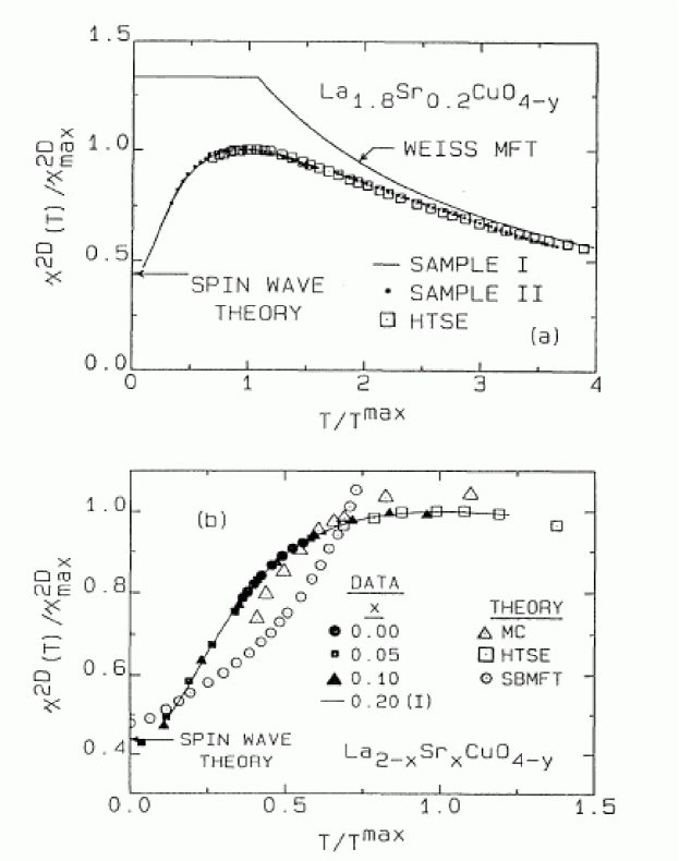
Figure 1: Cu²⁺ sublattice susceptibility $\chi^{2D}(T)/\chi^{2D}_{max}$ vs $T/T^{max}$ for five different samples of La_2-zSr_zCuO_4-y with effective doping levels $x=z-2y=0.0$, $x=0.05$, $x=0.1$, $x=0.13$, and $x=0.2$, compared with theoretical 2D Heisenberg calculations and the Weiss molecular-field (MFT) prediction. Reproduced with permission from [2].

To explain the scaling behavior of Eq.(1), Johnston[2] introduced a doping-dependent 2D Heisenberg exchange constant, $J(x)$, and the ratio

$$R(x)=\frac{\chi^{m}(x)}{\chi^{m}_{calc}(x)}\,,$$ (2)

where $\chi^{m}_{calc}(x)$ is the result obtained for the 2D Heisenberg model for a given $J(x)$. He found that $R(x)$ gradually decreases from $R(x=0)=1$ to $R(x=0.2)\simeq 0$ (Fig.2).

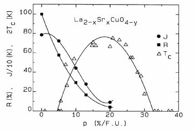
Figure 2: Effective intralayer Cu-Cu exchange constant $J$ and the ratio $R=\chi^{2D}_{max}/\chi^{2Dcalc}_{max}$ vs. hole doping $p=x$. $T_{c}(p)$ is shown for comparison. The solid curves are guides to the eye. Reproduced with permission from [2].

Oda et al.[12] confirmed Johnston’s scaling law for the bulk spin susceptibility in Sr- and Ba-doped La₂CuO₄, and extended its applicability to the 2212 family of cuprates, Bi₂Sr_3-yCa_y-xCu₂O₈. The experimental results for both families displayed excellent data collapse to the theoretical 2D Heisenberg curve. Like Johnston, Oda et al. found that the weight of the Heisenberg-like contribution decreases with hole doping. To account for this decrease, Oda et al. introduced an effective magnetic moment,

$$\mu_{eff}=g\sqrt{s(s+1)}.$$ (3)

$g$ is defined in terms of $T^{m}(x)$ and $\chi^{m}(x)$ as

$$g^{2}(x)=11.6k_{B}\frac{T^{m}(x)\chi^{m}(x)}{N\mu_{B}^{2}}\,.$$ (4)

They found that both $T^{m}(x)$ and $g(x)$ decrease linearly with doping,

$$g(x)=2.2(1-4.5x)\propto T^{m}(x).$$ (5)

The magnitude of $g(x)$ is that expected from the sum rule for a homogeneous material,

$$\int_{0}^{\infty}\frac{d\omega}{2\pi}\,\int\frac{d^{3}q}{(2\pi\hbar)^{3}}(\chi(\omega,\bm{q},x)-\chi_{0}(x))=g^{2}(x)\frac{s(s+1)}{3}\,,$$ (6)

but we caution the reader that homogeneity may not be present in the underdoped regime.

Both the doping dependence of the $x$-dependent Fermi liquid part and the temperature dependent spin liquid component were found by Oda et al. to be in good agreement with earlier results of Johnston[2]; like Johnston they found that the temperature-dependent scaling part of the bulk spin susceptibility disappears at some critical doping value; according to Eq.(5), that is $x\simeq 0.22$.

Another early study of bulk susceptibility in La_2-xSr_xCuO₄ was performed by Yoshizaki et al. [29], who give a plot of $T^{m}(x)\simeq 1000K(1-4.5x)$, without attempting Johnston scaling. Since $1000K$ does not match the value of the exchange coupling $J$ in the insulator, Yoshizaki et al. found a jump in $T^{m}(x)$ at the MI boundary.

Further confirmation of Johnston scaling of the form Eq.(1) for the bulk spin susceptibility in the 2-1-4 family was obtained by Nakano et al. [11] (Fig. 3), who demonstrated an excellent data collapse for a number of samples of La_2-xSr_xCuO₄, both in the underdoped region and that close to and beyond optimal doping. Nakano et al. arrived at their scaling law by assuming the presence of additional temperature-dependent terms: an impurity Curie term $C/T$ and a linear term $B(T-T_{a})$ in the underdoped and overdoped regimes. They did not attempt to fit the 2D Heisenberg model calculations; an empirical scaling data collapse was constructed instead, with results that were in agreement with Oda et al.[12].

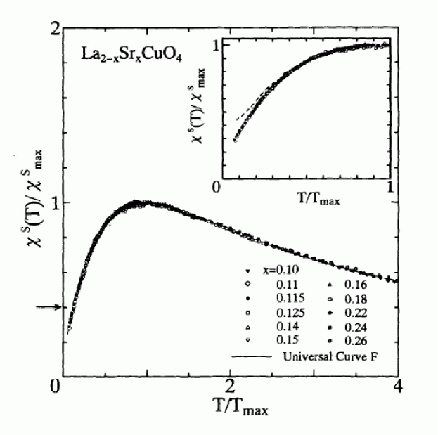
Figure 3: $\chi^{S}(T)/\chi^{S}_{max}$ versus $T/T_{max}$ for the superconducting samples of La_2-xSr_xCuO₄. The arrow shows the value of $\chi^{S}(T=0)/\chi^{S}_{max}$ predicted by the 2D Heisenberg model calculations. The solid line is the universal curve. The inset shows that the universal curve decreases more rapidly for $T\ll T_{max}$ than that obtained by Johnston[2] (dashed line). Reproduced with permission from [11]

An alternative form of scaling for the bulk spin susceptibility was proposed by Levin and Quader[30]. Similar to the studies reviewed above, they suggested separation of the bulk spin susceptibility in two components, the temperature-independent Fermi liquid component and the scaling component. However, in their model the scaling component originates from the contribution of a separate itinerant band. Levin and Quader[30] took the 2D density of states in the following form:

$$\nu(\epsilon)=\nu_{\xi}+\nu_{\eta}\theta(-\epsilon),$$ (7)

where the index $\xi$ corresponds to a large hole band, which produces the usual Fermi liquid term in the bulk spin susceptibility. The chemical potential $\mu$ lies very close to the top of the second band $\eta$ and enters that band at $x=x_{0}$. The contribution of the band $\eta$ to the bulk spin susceptibility becomes temperature-dependent due to thermally activated carriers and is a universal function $\chi_{\eta}(\Gamma(x-x_{0})/T)$, where $\Gamma\propto\nu_{\xi}^{-1}$ is a Fermi liquid parameter. The parameter $\Gamma(x-x_{0})$ is thus an analog of $T^{m}(x)$. The two-band model produced a reasonably successful data fit for the bulk susceptibility in TlSr₂(Lu_1-xCa_x)Cu₂O_y for both the underdoped and the overdoped regimes.

To summarize, the various independent measurements of the bulk susceptibility in the 2-1-4 and 1-2-3 materials can now be seen to be consistent with one another and with the picture first set forth by Johnston: that in the underdoped regime, for dopings between $x\sim 0.06$ and $\sim 0.22$, and $T>T^{m}/3$, one has two independent contributions to the bulk spin susceptibility. One comes from a 2D Heisenberg spin liquid with a doping-dependent effective interaction, $J_{eff}(x)\sim T^{m}(x)$; the second represents a Fermi liquid contribution whose strength increases as the doping level is increased. As we shall see, the fall-off of the rescaled spin susceptibility below the Heisenberg spin liquid value at $T\sim T^{m}/3$ appears to be a universal property of the spin liquid in the cuprates.

2.2 Measurements of the bulk susceptibility using the NMR Knight shift

The Knight shift seen in NMR experiments is a measurement of the bulk spin susceptibility at a particular nuclear site[31], so that measurements of the Knight shift for different nuclei serve to supplement direct measurements of the bulk susceptibility. Most of the early analysis of the NMR data used a single-component Mila-Rice-Shastry (MRS) description[32] for which the justification was the observation by Alloul et al.[14] and Takigawa et al.[33] that the ${}^{63}Cu$, ${}^{17}O$ and ${}^{89}Y$ Knight shifts in YBa₂Cu₃O₇ and YBa₂Cu₃O_6.63 have the same anomalous temperature dependence (Fig.4). MRS proposed a hyperfine Hamiltonian that described the coupling of a single magnetic component formed by the system of planar Cu²⁺ spins and holes mainly residing on the planar copper sites to the various nuclei. Most earlier Knight shift experiments[33, 34] confirmed this one-component Zhang-Rice[35] singlet picture, which is basically correct for the parent insulator. However, as first noted by Walstedt et al.[36] in connection with spin-lattice relaxation rate measurements, and discussed in detail below, the single component description turns out to lead to a number of contradictions in the doped materials, and requires modification.

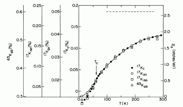
Figure 4: The experimental planar Cu and O Knight shifts in YBa₂Cu₃O_6.63 plotted vs the temperature $T$. The values for the static planar susceptibility $\chi_{0}(T)/\mu_{B}^{2}$ are given on the right-hand scale. Different Knight shifts and the static spin susceptibility have the same temperature dependence. Reproduced with permission from [34].

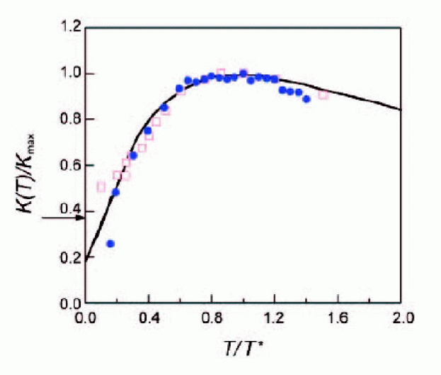
Figure 5: The spin shift in YBa₂Cu₄O₈ versus $T/T^{m}$, showing the applicability of Johnston/Nakano scaling and the relevance of the 2D Heisenberg model[15]. The solid line is taken from Ref. [11], the dotted green line is the calculated susceptibility of the spin-1/2 2D Heisenberg antiferromagnet[5] and the data points are taken from Ref.[37]. The arrow points to the zero-temperature prediction for the 2D Heisenberg antiferromagnet. Reproduced with permission from [15].

Just as was the case for the bulk spin susceptibility, the temperature-dependent Knight shift data for different doping levels and different families of cuprates displays Heisenberg model-type scaling. The ${}^{89}Y$ Knight shift data from Alloul et al.[14] for different doping levels in the 1-2-3 family has been scaled to a single curve with very good data collapse by Wuyts et al.[13], although no comparison to the 2D Heisenberg model or the Nakano et al.[11] bulk spin susceptibility scaling curve was provided. Recently Curro et al.[15] and the authors[3] have shown that the two are consistent; as may be seen in Fig.5, the NMR Knight shift follows very well the Johnston-Nakano bulk susceptibility scaling form and the Heisenberg model for the 1-2-4 member of the 1-2-3 family. Spin liquid scaling behavior determined by $T^{m}(x)$ has thus been shown to be universal in the cuprates.

What then is the direct experimental evidence from Knight shift measurements for the presence of two distinct components? One material for which a contradiction with the simple one component model was found is YBa₂Cu₄O₈, where a more precise measurement[38] of the copper Knight shift data in magnetic fields parallel to the c-axis, ${}^{63}K_{\parallel}$, found that it displays a rather unusual temperature dependence, one that is different from that seen for the bulk spin liquid susceptibility. A second example comes from quite recent measurements by Haase et al.[39] of the planar and apical oxygen Knight shifts for La_1.85Sr_0.15CuO₄. As we discuss in a later section, these indicate that while the temperature-dependent part of the Knight shift on different nuclei is indeed the same, there is a temperature-independent part of the Knight shift above the superconducting temperature, $T_{c}$, that is different for the planar copper and the planar and apical oxygen nuclei. The key signature of this effect, the deviation of various Knight shifts from the same temperature dependence at temperatures below $T_{c}$, is clearly visible in Fig.4. These contradictions suggest that the original MRS hyperfine Hamiltonian has to be modified to include these new effects, and that the one-component spin dynamics and the Zhang-Rice singlet picture[35] fails at moderate doping levels[36], a topic to which we return in Section 3.

2.3 Spin-lattice relaxation rates

In the MRS Hamiltonian that is described in detail in the following section, wave vector dependent form factors arise from the presence of a transferred hyperfine interaction between the Cu spins and the probe nucleus. For probe nuclei other than copper, these vanish at the commensurate wave vector $\bm{Q}=(\pi,\pi)$, so that, for example, an in-plane oxygen nucleus will feel little of a spin response that is peaked at the commensurate wave vector. (That this should be the case is obvious if one recalls that such oxygen are located midway between copper nuclei, and for an antiferromagnetic array of copper spins, the nearest neighbor spins would cancel one another out in their influence on the oxygen site.) The striking difference of the temperature dependence and magnitude of the spin-lattice relaxation on the ${}^{63}Cu$, ${}^{17}O$, and ${}^{89}Y$ nuclei led Millis, Monien, and Pines (MMP)[40] to the conclusion that a localized or nearly localized spin component of the dynamic magnetic response function must be strongly peaked at the commensurate wave vector, as might be expected if one were close to an antiferromagnetic instability.

Indeed, closer study shows that even a slight deviation from commensurability within the MMP approach based on the MRS one-component model will have a significant impact on oxygen relaxation rates that is not seen experimentally[40]. Thus, an incommensurate peak structure for $\chi^{\prime\prime}(\bm{q},\omega)$, such as has been inferred from inelastic neutron scattering (INS) experiments[41, 42] on the 2-1-4 materials, is inconsistent with this approach. One way to get around this difficulty is to introduce additional transferred hyperfine interactions[43]; a second way, proposed by Slichter[44, 45] , is to note that unlike NMR, INS is a global probe of spin excitations, so that a suitable domain structure (regions of commensurate near-antiferromagnetic behavior, separated by domain walls) would give rise to the apparent incommensuration inferred from the INS experiments. We adopt this explanation in what follows.

The spin fluctuation response function proposed by MMP was that appropriate to any spin liquid near a commensurate antiferromagnetic instability:

$$\chi_{SL}(\bm{q},\omega)=\frac{\chi_{\bm{Q}}}{1+\xi^{2}(\bm{q}-\bm{Q})^{2}-i\frac{\omega}{\omega_{SF}}\,}\,,$$ (8)

where the peak susceptibility takes the form,

$$\chi_{\bm{Q}}=\alpha\xi^{2},$$ (9)

with $\xi$ as the magnetic correlation length, and $\alpha(x)$ as a temperature-independent constant. The copper NMR ${}^{63}T_{1}$ and ${}^{63}T_{2G}$ relaxation rates provide a direct measure of the strength and character of the spin liquid response function, measuring as they do the momentum-integrated imaginary and real part of the spin response function, $\chi_{SL}(\bm{q},\omega)$[46]. One finds:

$$\frac{1}{{}^{63}T_{1}}\, \propto \frac{\alpha T}{\omega_{SF}}\,,$$ (10)

$$\frac{1}{{}^{63}T_{2G}}\, \propto \alpha\xi.$$ (11)

Imai et al.[18] in an early scaling analyses (Fig. 6) of the copper relaxation rates for the 2-1-4 family demonstrated experimentally the existence of a universal high temperature limit for ${}^{63}T_{1}$ that is temperature- and doping- independent:

$$\frac{1}{{}^{63}T_{1}(T,x)}=const,$$ (12)

which according to Eq.(10) means that at high temperatures the spin fluctuation energy, $\omega_{SF}$ must be proportional to T. This universal high-temperature behavior of ${}^{63}T_{1}$ was explained in terms of the QC (Quantum Critical)[46, 9] behavior seen in the sigma-model[47, 48] that, strictly speaking, is only applicable to the parent insulating compound. Indeed the empirical finding of a temperature- and doping independent ${}^{63}T_{1}$ in the 2-1-4 family of materials extends to temperatures much higher than those at which such a theoretical explanation would apply.

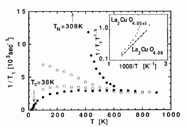
Figure 6: Temperature dependence of $1/^{63}T_{1}$ measured by NQR for La_2-xSr_xCuO₄ ($x=0$, $x=0.04$, $x=0.075$, $x=0.15$). The inset shows a semilogarithmic plot of $1/^{63}T_{1}T^{3/2}$ (in units of $sec^{-1}K^{-1.5}$) vs $1000/T$ for the clean sample of La₂CuO_4.00 and for La₂CuO_4.00+δ. The solid curve is the best fit to the theoretical prediction of 2D Heisenberg model. Reproduced with permission from [18]

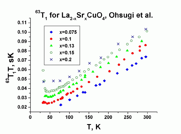
Figure 7: At high temperatures the dependence of ${}^{63}T_{1}T$ on temperature in La_2-xSr_xCuO₄[49] for different doping levels represents a set of parallel lines.

Two other high-temperature forms for the relaxation rates based on $z=1$ and $z=2$ dynamical scaling were therefore suggested[46, 9] on the basis of the non-linear sigma model[47, 48] and general scaling arguments, and verified experimentally. In $z=1$ scaling, $\omega_{SF}$ and $\xi$ are related by

$$\omega_{SF}\propto\Delta=\frac{c}{\xi}\,,$$ (13)

so the presence of $z=1$ QC scaling in the underdoped materials leads to the simple results:

$$\frac{{}^{63}T_{1}T}{{}^{63}T_{2G}}\,\propto\omega_{SF}\xi\propto c$$ (14)

On the other hand, for $z=2$ (mean field) scaling one has

$$\omega_{SF}=\frac{\Gamma}{\xi^{2}}\,,$$ (15)

so that if it is present one finds

$$\frac{{}^{63}T_{1}T}{{}^{63}T_{2G}^{2}}\,\propto\omega_{SF}\xi^{2}=\Gamma.$$ (16)

The NMR experimental results of Curro et al.[37] show that both forms of scaling are present in the material, YBa₂Cu₄O₈. At high temperatures, for $T>T^{m}\sim 500K$, Eq.(16) is valid and one has mean field behavior, while below $T^{m}$ the spin spectrum displays $z=1$ QC behavior down to a temperature $\sim 150K$, where the $T_{1}$ measurements suggest that a gap opens up in the spin liquid spectrum. We return to this finding below.

The relaxation rates for other nuclei, such as oxygen or yttrium, also display anomalous (i.e. non-Korringa) behavior, although in much milder form. A modified Korringa-type scaling for oxygen ${}^{17}T_{1}$ was suggested by MMP:

$${}^{17}T_{1}T\chi_{0}(T)=const.$$ (17)

Additional scaling forms have been proposed for the copper relaxation rates at lower temperatures. In particular, the authors[3] have observed recently that ${}^{63}T_{1}T$ reaches its universal high-temperature behavior with a different $x$-dependent offset (Fig.7),

$${}^{63}T_{1}T=BT+A(x),$$ (18)

where the constant $B$ is universal, while $A(x)$ changes linearly with doping, and its variation suggests the existence of a QC point in the spin liquid at $x_{0}\simeq 0.05$, where $A(x_{0})=0$. Eq.(18) shows excellent data collapse for the 2-1-4 and the 1-2-3 families.

An alternative form of scaling has been suggested to apply at moderate to low temperatures, $T<300K$, by Gor’kov and Teitel’baum (GT)[50] who found excellent data collapse (Fig.8) for the following scaling form:

$$\frac{1}{{}^{63}T_{1}}\,=\frac{1}{{}^{63}T_{1}(x)}\,+\frac{1}{{}^{63}\tilde{T}_{1}(T)}\,,$$ (19)

where $\tilde{T}_{1}(T)$ is a universal function for all high-T_c materials, while $\frac{1}{{}^{63}T_{1}(x)}\,$ varies with $x$. The suggested scaling form follows from the decomposition of relaxation rate into two different processes. The x-dependence of $1/^{63}T_{1}(x)$(Fig.9) looks rather unusual[50], since the proposed empirical disorder-driven relaxation rate, $1/^{63}T_{1}(x)$ decreases with increased doping $x$. The proposed GT scaling is assumed to be the result of intrinsic phase separation, and the pseudogap temperature $T^{*}(x)$ is proposed as a measure of the onset of such behavior.

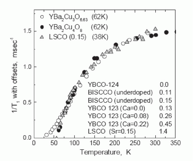
Figure 8: Temperature dependence of $1/^{63}T_{1}$ for YBa₂Cu₃O_6.63 overlaid with that for YBa₂Cu₄O₈ and La_1.85Sr_0.15CuO₄. In the lower right corner: the offset values for different compounds. Reproduced with permission from [50]

Figure 9: The offset $1/^{63}T_{1}(x)$ vs Sr content $x$ for LSCO (relative to that for YBa₂Cu₄O₈). The line is a visual guide. Reproduced with permission from [50].

2.4 Finite size effects

If scaling is present, it is natural to look for the possible presence of finite size effects, as Cho et al.[27] have done in the lightly doped La_2-xSr_xCuO₄ material. They found very good agreement with that expected for phase separation and domain formation on the insulating side of the Mott transition. However, there was no direct observation of the domain sizes of the different phases. According to finite-size scaling theory[51], the Neèl temperature for a domain of size $L$ takes the form,

$$1-\frac{T_{N}(L)}{T_{N}(L=\infty)}\,\propto L^{-1/\nu},$$ (20)

where $\nu=1/2$ in mean field theory. The experimental data can also be fit well by the expression

$$1-\frac{T_{N}(x)}{T_{N}(x=0)}\,\propto(x/x_{c})^{n},$$ (21)

with $n=1.90\pm 0.20\simeq 2$. Cho et al. conclude that

$$L(x)\propto\frac{1}{x}\,,$$ (22)

which means that the width of the domain wall is $x$ independent. They found that in the antiferromagnetic regime the scaling law takes the form:

$$\chi(x,T)=\chi(F(x)(T-T_{N}(x))),\ \ F(x)\propto\frac{1}{\left(x+\frac{C}{\xi_{0}(T_{N}(x))}\,\right)^{2}}\,.$$ (23)

Here $\xi_{0}(T)$ is the correlation length in the pure Heisenberg model,

$$\xi_{0}(T)=0.276a\exp{(2\pi\rho_{s}/k_{B}T)}\simeq 0.276a\exp{(J/k_{B}T)}.$$ (24)

2.5 Inelastic neutron scattering

Inelastic neutron scattering (INS) experiments enable one to explore the extent to which 2D Heisenberg model captures the momentum dependence and behavior at higher frequencies of the spin liquid as its properties are altered by doping. There is by now a vast body of literature that includes several recent reviews[52, 53, 54]. Our focus here is on the extent that the doped spin liquid continues to exhibit the quantum critical behavior inferred from the ultra low frequency dynamic properties measured in the NMR experiments described in the previous sections, and the ways in which departures from quantum critical behavior emerge as the frequency is increased into the multi-time range or one goes into the gapped normal or superconducting state. As we shall see, one of the most striking features that emerges with doping is the observation of peaks whose positions at lower frequencies reflect a doping-dependent incommensuration or discommensuration that indicates dynamic stripe formation; a second is the appearance of resonances and spin gaps in the normal state. Throughout this section we will be concerned, as we were in our discussion of NMR experiments, with possible universal behavior that is common to the 1-2-3 and 2-1-4 families.

2.5.1 $\omega/T$ scaling for the local spin susceptibility

Perhaps the most direct evidence of quantum critical scaling was provided by the INS measurements of the local (integrated) dynamic spin susceptibility. The remarkable results obtained in insulating and metallic low doped samples indicate the presence of the $\omega/T$ scaling expected in the vicinity of a $z=1$ quantum critical point.

Among early neutron scattering experiments that exhibit some form of scaling behavior those of particular interest are on lightly doped YBa₂Cu₃O_6+x by Birgeneau et al. [24], lightly doped La_2-xSr_xCuO₄ by Keimer et al. [23], and YBa₂Cu₃O_6.6 by Sternliebet al. [25]. Keimer et al.[23] and Birgeneau et al.[24] fit their experimental results for the local (integrated) spin susceptibility to the expression

$$\chi_{L}^{\prime\prime}(\omega)\equiv\int\frac{d^{2}q}{(2\pi)^{2}}\,\chi^{\prime\prime}(\bm{q},\omega)=C(\omega)tan^{-1}(a_{1}(\omega/T)+a_{2}(\omega/T)^{3}+\cdots)$$ (25)

The data collapse is good (Fig.10), but this form does not quite exhibit $\omega/T$ scaling because of the $T$-independent amplitude $C(\omega)$.

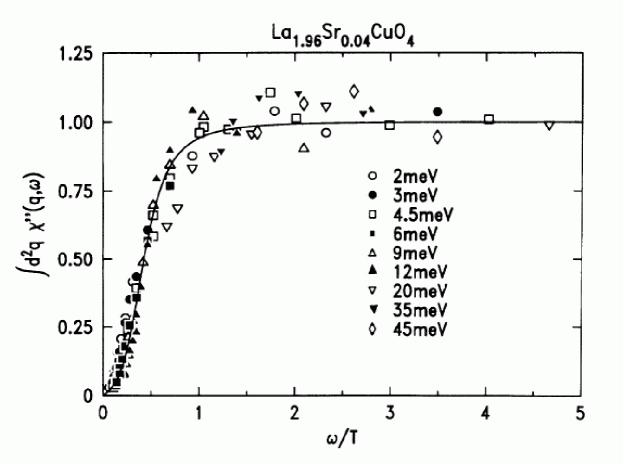
Figure 10: Normalized integrated spin susceptibility as a function of the scaling variable $\omega/T$. The solid line is the function $2/\pi\tan^{-1}[a_{1}\omega/T+a_{3}(\omega/T)^{3}]$ with $a_{1}=0.43$ and $a_{3}=10.5$. Reproduced with permission from [23].

Sternlieb et al. [25] subsequently found that true $\omega/T$ scaling exists for the local spin susceptibility in the underdoped material YBa₂Cu₃O_6.6. Their experimental results (Fig. 11) can be fit to the following simple scaling form:

$$\chi_{L}^{\prime\prime}(\omega,T)=A(x)\frac{\omega}{T}\,,$$ (26)

with a deviation from scaling that occurs at progressively lower temperatures, as the frequency $\omega$ increases.

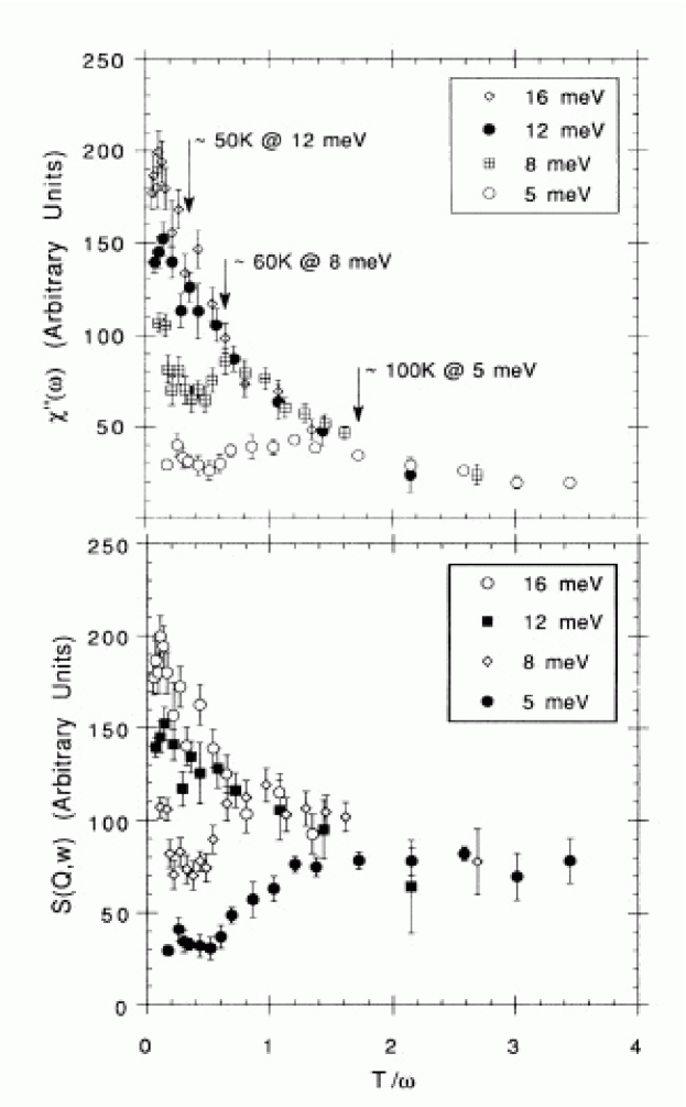
Figure 11: (top) The temperature dependence of the local dynamic spin susceptibility $\chi^{\prime\prime}(\omega)$ for a fixed energy transfers converges to a universal function of $T/\omega$ at high temperatures. The arrows show the temperature above which the scaling behavior occurs. (bottom) The corresponding scattering function $S(\omega)$ vs $T/\omega$. Reproduced with permission from [25].

In more recent experiments, Bao et al.[55] studied experimentally the destruction of 2D antiferromagnetic order in $Li$-doped La₂CuO₄. Since holes are loosely bound by $Li$ impurities, the doped material remains an insulator even when long-range order is destroyed at $x>0.03$. However, unlike the superconducting La_2-x(Sr,Ba)_xCuO₄, there are no additional complications due to the presence of mobile doped holes, making possible a cleaner measurement of the spin dynamics. Bao et al.[55] found a commensurate energy spectrum of spin excitations at $x>0.03$, where the long-range order is not present, and a characteristic quantum critical $\omega/T$ scaling for the local spin susceptibility (Fig. 12). The scaling function, however, is different from that obtained by Sternliebet. al.[25] In particular, Bao et al.[55] found significant deviations of the scaling function from linearity, with

$$\chi^{\prime\prime}_{L}(\omega,T)=\chi_{\pi}f(\omega/T),$$ (27)

and

$$f(x)=\frac{0.18x}{0.18^{2}+x^{2}}.$$ (28)

Below $T=50K$ this scaling changes to one with a constant energy scale $\Gamma_{0}=1meV$,

$$\chi^{\prime\prime}_{L}(\omega,T)=\chi_{\pi}g(\omega/\Gamma_{0}),$$ (29)

where

$$g(x)=\frac{x}{1+x^{2}}.$$ (30)

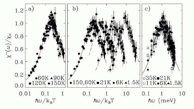
Figure 12: (a) $\omega/T$ scaling is valid for La₂Cu_0.94Li_0.06O₄ in the high temperature QC regime The solid line is the scaling function, Eq.(28). (b) $\omega/T$ scaling becomes invalid in the low temperature regime. (c) A new scaling for the low temperature regime, with a constant energy scale $\Gamma_{0}=1meV$. The solid line is the scaling function Eq.(30). Reproduced with permission from [55].

Stock et al.[56] recently confirmed the low-frequency $\omega/T$ scaling for $\chi^{\prime\prime}_{L}(\omega,T)$ in oxygen ordered ortho-II YBa₂Cu₃O_6.5 superconductor found earlier in this material in the oxygen-disordered state by Birgeneau et al.[24]. Stock et al. fit their expression to the form Eq.(25), with only a linear term in $\omega/T$ present. They find that the $\omega/T$ scaling breaks down at higher frequencies, $\omega>20meV$, since the amplitude $C(\omega)$ in Eq.(25) becomes temperature-dependent.

2.5.2 Temperature and frequency dependence of the correlation length

Keimer et al.[23] find evidence for finite size scaling, since a good fit to their experimental results can be obtained with the following expression for the correlation length:

$$\xi^{-1}(x,T)=\xi^{-1}(x,T=0)+\xi^{-1}(x=0,T),$$ (31)

with $\xi(x,T=0)\propto 1/x\propto L$, where $L$ is the size of the domain for finite size scaling.

Eq.(31) was later generalized to finite frequencies $\omega$ by Aeppli et al.[26], who fit their results for the correlation length in La_1.86Sr_0.14CuO₄ (Fig.13) to the following form:

$$\xi^{-1}(T,\omega)=\sqrt{\xi^{-2}(0)+\omega^{2}+T^{2}}.$$ (32)

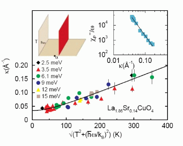
Figure 13: Temperature dependence of the inverse correlation length $k(\omega,T)$ at various fixed energy transfers plotted against $\sqrt{(\hbar\omega/k_{B})^{2}+T^{2}}$. The solid line corresponds to a $z=1$ QCP. The graph in the upper right shows how the peak response depends on $k=k(\omega=0,T)$. The inset in the upper left shows the 3D space defined by $(\omega,T)$ phase space probed by the $x=0.14$ sample, and the solid circle represents the nearby QCP. Reproduced with permission from [26].

2.5.3 Direct measurements of $\chi^{\prime\prime}(\bm{q},\omega)$

Inelastic neutron scattering experiments provide a direct measurement of the spectrum of spin excitations, and thus of the spin wave velocity and exchange couplings in the antiferromagnetic insulator[57, 58, 59]. We shall see that the detailed measurements of the spectrum of the spin excitations in underdoped high-temperature superconductors that have recently been carried out for both the 2-1-4[60, 61, 62, 63] and the 1-2-3[64, 65, 66] families provide evidence for its universality.

Incommensuration/Discommensuration

Early neutron measurements on both the 2-1-4 and the 1-2-3 families of high-temperature superconductors revealed an incommensurate spectrum of spin excitations at low frequencies. Cheong et al.[41] and Mason et al.[42] discovered in their inelastic neutron scattering measurements on the 2-1-4 family of materials that the position of the low-energy spin fluctuation peak shifts from $(\pi,\pi)$ in the parent insulating compound to $(\pi\pm 2\pi\delta,\pi)$ and $(\pi,\pi\pm 2\pi\delta)$ in the underdoped superconductor. They found that the incommensurability $\delta$ in the underdoped regime grows approximately linearly with increased hole concentration $x$, $\delta\simeq x$, at least for $x<0.12$. For $x>0.12$, the incommensurability $\delta(x)$ saturates at a finite value. Incommensurate peaks in the spin response function $\chi^{\prime\prime}(\bm{q},\omega)$ at low frequencies were also discovered in the bilayer system YBa₂Cu₃O_6+x[67]. As Mook et al.[67] have first shown, the incommensurate peaks in the bilayer system are located at the same positions as in the single-layer La_2-xSr_xCuO₄ system at similar level of hole doping. Thus, they concluded that the band structure, which is very different in these two families of materials, plays a minor role in the spectrum of spin excitations at low frequencies. In what follows we will refer to these peaks as reflecting incommensurate behavior, although, as noted earlier, for these results to be consistent with NMR, these should rather be regarded as reflecting discommensuration, or dynamic stripe order.

Wakimoto et al.[68] and Matsuda et al.[69] extended the measurements of $\chi^{\prime\prime}(\bm{q},\omega)$ in La_2-xSr_xCuO₄ to the spin glass regime, $0.02<x<0.055$. They found that while the low-energy spin excitations remain incommensurate with the same $\delta\simeq x$ as in the metallic phase, the positions of the incommensurate peaks are rotated by $\pi/4$ relative to those in the metal, as shown in Fig.14. Unlike in metallic phase, the diagonal stripe structure for the insulating spin glass phase is seen as Bragg peaks in elastic scattering measurements and thus is static at low temperatures[69]. Moreover, the incommensurability of the spin fluctuations disappears at higher frequencies or temperatures, above a certain energy threshold for the incommensurate structure, which we shall see is directly related to the spin gap.

An interesting linear scaling relationship between the incommensurability $\delta(x)$ and the superconducting temperature, $T_{c}(x)$, was suggested by Yamada et al.[70]. which, they find, holds extremely well for the 2-1-4 family of materials in the underdoped regime, $T_{c}(x)=\hbar\nu*_{214}\delta(x)$, with $\hbar\nu*_{214}\simeq 20meV\AA$. Balatsky and Bourges[71] and Dai et al.[72] found that Yamada scaling is also applicable to the 1-2-3 family of materials, with $T_{c}(x)=\hbar\nu*_{123}\delta(x)$ and $\nu*_{123}\simeq 36.6meV\AA$[72]. Since the maximum of $T_{c}$ is different in different families of cuprates, while the incommensurability is universal and depends only on hole doping, $\nu*$ is different for different families of materials.

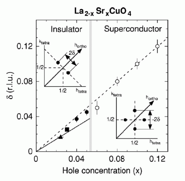
Figure 14: Hole concentration $(x)$ dependence of the splitting of the incommensurate peaks $(\delta)$ in La_2-xSr_xCuO₄ in tetragonal reciprocal lattice units. Open circles indicate the data for the inelastic incommensurate peaks reported by Yamada et al.[70]. Filled circles and square are the data for elastic incommensurate peaks reported by Wakimoto et al.[68]. The broken and solid lines correspond to $\delta=x$. The insets show the configuration of incommensurate peaks in the insulating phase (diagonal stripe) and the superconducting phase (collinear stripe) Reproduced with permission from [69].

Stock et al.[56] considered the applicability of Yamada scaling to both 2-1-4 and 1-2-3 families of high-temperature superconductors. They plotted the incommensurability $\delta$ as a function of $T_{c}(x)/T_{c}^{max}$, a quantity proportional to the number of holes in the plane in the underdoped regime (see Fig.15). Their plot thus confirms for the 2-1-4 materials the conclusion of Mook et al.[67] that the incommensurability of low-energy spin fluctuations in cuprate superconductors depends only on hole concentration in the plane, and not a particular material or band structure.

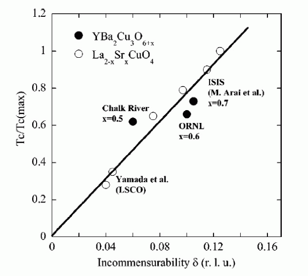
Figure 15: Reduced superconducting temperature $T_{c}/T_{c}(max)$ as it relates to the incommensurability $\delta$ in YBa₂Cu₃O_6+x and La_2-xSr_xCuO₄. Reproduced with permission from [56].

High-energy spin excitations and the resonance peak

Early INS studies of high-frequency spin fluctuations were limited due to poor resolution. Many of these measurements were initially done on the 1-2-3 family of materials, where the resonance peak[73, 74] enhances spin response at higher energies. The resonance peak in the 1-2-3 family of materials corresponds to a sharp enhancement of the intensity of commensurate spin excitations at high frequencies near the frequency, $E_{res}(x)$, that depends on hole doping $x$. The observation then raised the question of whether the peak was a consequence of spin gap in the fermionic excitations or was an intrinsic property of the spin liquid in the vicinity of $(\pi,\pi)$.

At first the resonance was only observed in the superconducting state. Since the resonance peak was not observed in the inelastic neutron scattering experiments on the 2-1-4 family, this led to an explanation that this feature most likely arises as a result of the coupling of spin excitations to fermions with a d-wave gap or d-wave like gap in the normal state. Indeed, Dai et al.[74] found that the resonance peak first appears above $T_{c}$ at $T^{*}(x)$, which decreases with increased hole doping, the resonance energy $E_{res}(x)$ increases with increased doping and tracks the doping dependence of $T_{c}(x)$, as shown in Fig.16.

However, more detailed neutron scattering studies revealed that the resonance corresponds to a special frequency at which high-energy spin excitation spectrum becomes commensurate. As we have seen above, the spin excitation spectrum depends only on hole doping, and not on a particular material, a conclusion that casts doubt on the quasiparticle gap explanation of the resonance. Inelastic neutron scattering studies near the resonance frequency were first done by Bourges et al.[75, 76] in the YBa₂Cu₃O_6.5 material. Bourges et al. found that the commensurate resonance peak was broadening in momentum, both above and below the resonance frequency $E_{res}$. Based on their findings, Bourgeset al. suggested that the spin excitations disperse at high frequencies in a way that is similar to that expected for spin waves in the parent insulating compound. Arai et al.[77] later studied the momentum dispersion of spin excitations near the resonance peak in YBa₂Cu₃O_6.7 in more detail. They found evidence for two modes that meet near the resonance energy, one that opens downwards and gives rise to incommensurate spin excitations at low energies, the other, a new mode that opens upwards in energy, giving rise to spin wave-like dispersive excitations at high energies. Arai et al. found that the two modes meet at the frequency $\omega\simeq 41meV$, slightly above the characteristic resonance frequency $E_{res}=36meV$ for their material. More recent INS experiments on YBa₂Cu₃O_6.5[65], YBa₂Cu₃O_6.6[64] and YBa₂Cu₃O_6.95[66], however, suggest that the high energy mode and the low energy mode meet at the resonance frequency.

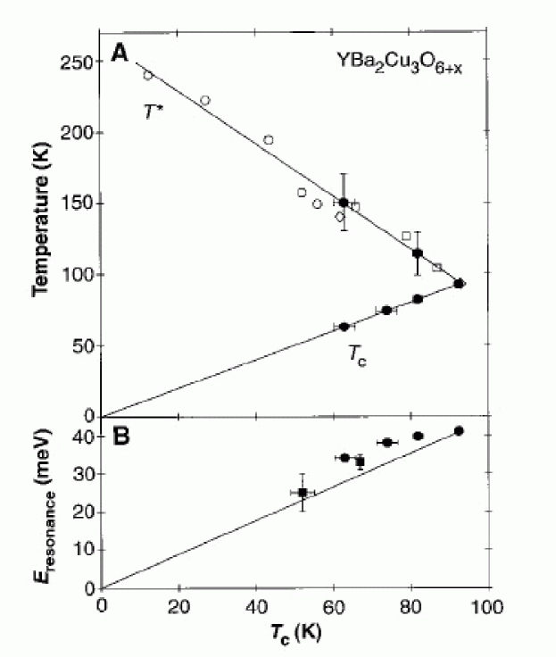
Figure 16: $T^{*}$ and the resonance energy $E_{resonance}$ as a function of $T_{c}$ in YBa₂Cu₃O_6+x. The open circles and open squares are temperatures at which $d\rho(T)/dT$ reaches broad maximum. The open diamonds show the pseudogap temperature $T^{*}$ determined from NMR measurements[33]. The filled circles correspond to $T_{c}$ and $T^{*}$, where the resonance first appears in INS measurements. Filled squares are from Fong et al.[73]. Horizontal error bars are superconducting transition widths. The solid lines are guides to the eye. Reproduced with permission from [74].

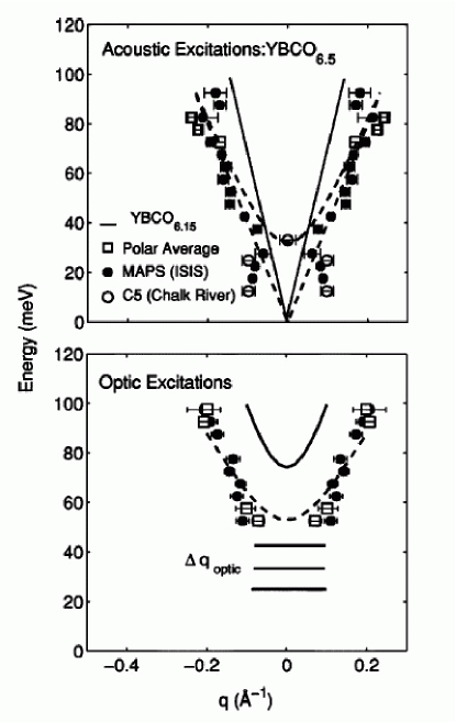
Figure 17: The dispersion of acoustic and optic modes in YBa₂Cu₃O_6.5 with respect to commensurate $(\pi,\pi)$ position at $T=6K$. The filled circles are from two Gaussian fits along the $[100]$ and $[010]$ directions above the resonance energy and from $[100]$ direction below the resonance energy. The open circles represent the positions of the incommensurate peaks found in experiments conducted at Chalk River. The open squares represent the peak position that results from a polar average around $(\pi,\pi)$ position. The solid lines schematically represent the dispersion of the insulating compound as measured by Hayden et al.[58]. The dashed lines are fits of the high-energy dispersion to linear spin wave theory for $\omega>40meV$. The horizontal bars show the q-width observed for three optic scans at constant energy. Reproduced with permission from [65].

A typical energy spectrum of the spin excitations as measured by Stock et al.[65] in a detwinned ortho-II sample of YBa₂Cu₃O_6.5 is shown in Fig.17. As Mook et al.[78] had found earlier for a detwinned sample of YBa₂Cu₃O_6.6, Stock et al. found two, rather than four incommensurate peaks below the resonance frequency $E_{res}=33meV$. This result strongly suggested a one-dimensional character for the spin fluctuations, consistent with the formation of dynamic stripes[79, 61]. The incommensurability $\delta$ observed at low frequencies decreased with increased energy transfer and disappeared at $\omega=E_{res}$. The spin excitations started to disperse outward again at high frequencies, $\omega>E_{res}$. Stock et al.[65] found the dispersion for acoustic spin excitations to be isotropic and similar to the spin waves in the insulator, as shown in Fig.18; they fit their results to a gapped spectrum,

$$\epsilon_{ac}(q)=\sqrt{\Delta_{ac}^{2}+(c\bm{q})^{2}},$$ (33)

with $\Delta_{ac}\simeq E_{res}\simeq 33meV$ and a spin wave velocity $c\simeq 365meV\AA$, which is close to the value $c\simeq 400meV\AA$ obtained from the slope of high energy spin excitations. The spin wave velocity is dramatically reduced from its value in the insulator, $c\simeq 650meV\AA$[58].

Stock et al. also measured the width of the ring of high energy spin wave excitations and found that it increased linearly with frequency at low temperatures. The low-energy spectral weight was dominated by the resonance peak at $E_{res}=33meV$, which had an asymmetric shape, with a quick drop-off of intensity for $\omega>E_{res}$ and a much slower reduction at $\omega<E_{res}$. Stock et al.[56], however, estimated that the resonance represented only 3 % of the total spectral weight of spin excitations; most of its spectral weight would appear only at higher energies. Similar to spin waves in the insulating compound, $\chi"_{L}(\omega)$ approached a constant at high energies $\omega>E_{res}$, $\chi"_{L}(\omega>E_{res})\simeq 5-7\mu_{B}^{2}/eV$, somewhat reduced from a similar value for the insulator, $7-8\mu_{B}^{2}/eV$[65].

A very similar dispersion for spin excitations was found by Rezniket al.[66] in a twinned sample of YBa₂Cu₃O_6.95. They observed four incommensurate peaks dispersing inward with increased frequency at frequencies below the resonance frequency $E_{res}=41meV$ and becoming commensurate at the resonance frequency. The dispersion of spin excitations was cut off below the resonance frequency at a characteristic spin gap frequency $E_{gap}\simeq 33meV$. Reznik et al. concluded that their data was consistent with the isotropic gapped spin wave-like excitations dispersing outward at frequencies above the resonance frequency. As had Stock et al., Reznik et al. found the $\bm{q}$-integrated intensity to be approximately constant at high frequencies $\omega>E_{res}$, as expected for spin wave-like excitations. Because of resolution problems, Reznik et al. were not able to calibrate their data in absolute units, or estimate the spin wave velocity.

Not all INS studies have found spin wave-like excitations with a reduced effective exchange coupling $J$ at high energies. For example, Hayden et al.[64] performed measurements in a twinned sample of YBa₂Cu₃O_6.6 with effective hole doping $x\simeq 0.1$ close to the $x=1/8$ stripe ordering instability. As had other groups, Hayden et al. observed incommensurate spin excitations that dispersed inward up to resonance frequency $E_{res}\simeq 34meV$. However, their measurements at frequencies above $E_{res}$ indicated a strikingly different picture. Instead of the gapped spin waves found by other groups, Hayden et al. resolved four peaks at $\omega>E_{res}$ rotated by 45 degrees that dispersed outward in energy. Their measured dispersion for spin excitations is consistent with that observed earlier in stripe-ordered materials, such as La_2-xNi_xCuO₄[79] and La_1.875Ba_0.125CuO₄[61]. Hayden et al.[64] found little dispersion of the rotated incommensurate peaks at high energies, $66meV<E<105meV$. This led them to conclude that the high-energy spectrum of spin excitations they measured was inconsistent with commensurate gapped spin wave spectrum observed by other groups.

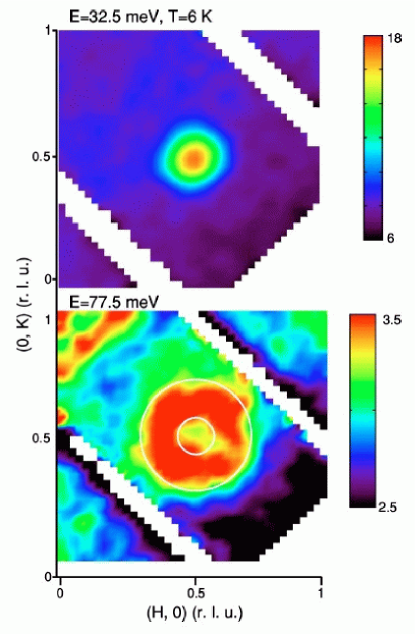
Figure 18: Smoothed two-dimensional slices through the correlated response at $32.5meV$ and $77.5meV$ energy transfers and integrated $\pm 7.5meV$ along the energy axis in YBa₂Cu₃O_6.5. At $77.5meV$ the ring of scattering shows the intersection of the cone of spin wave dispersion emanating from the $(1/2,1/2)$ position with a constant energy surface. Within statistics the velocity is isotropic. The intensity is represented by false color. Reproduced with permission from [65].

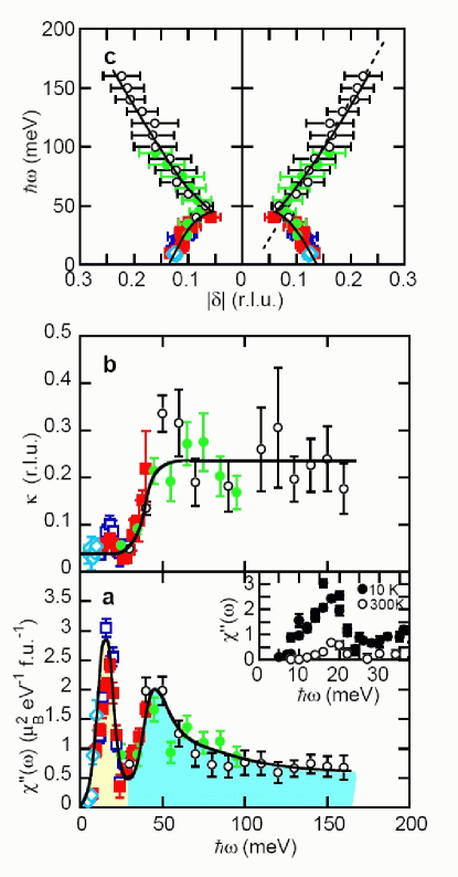
Figure 19: Magnetic excitation spectrum and evolution of the form of the magnetic response with energy. Symbols indicate different incident energies, open diamonds: $E_{i}=30meV$, open squares: $E_{i}=55meV$, filled squares: $E_{i}=90meV$, filled circles: $E_{i}=160meV$, open circles: $E_{i}=240meV$. ”peak-dip-hump” structure in the integrated susceptibility $\chi^{\prime\prime}(\omega)$ suggesting that the magnetic response has two components. The inverse correlation length $k(\omega)$ shows significant broadening at high energies. Reproduced with permission from [63].

High energy spin excitations have also been studied in several materials belonging to the 2-1-4 family. The question of the renormalization of the effective exchange coupling $J$ and the spin wave velocity $c$ of the insulator by doped carriers was first investigated by Hayden et al.[60] for La_1.86Sr_0.14CuO₄ in high-energy transfer inelastic neutron scattering experiments. They found that the spectrum of spin excitations at high energies fits the Heisenberg model well, with an effective exchange coupling $J$ that is only mildly reduced from its value in the insulator: for this material, $J_{eff}=130meV$, $Z_{\chi}=0.15$, values that are somewhat reduced from the corresponding values in the insulator, $J=153meV$, $Z_{\chi}=0.39$. They concluded that quantum fluctuations increase, but that at the high energies they study, $J$ and $c$ do not get strongly renormalized by doped holes. However, the spectral weight of their measured high-energy spin excitation decreases very strongly from its value at $x=0$; the peak of that weight for $x=0.14$ was found[60] to be at $\omega\simeq 22meV$, significantly below the corresponding peak for the insulating compound. The details of the spin excitation spectrum at low energies, however, could not be resolved.

More recent high resolution inelastic neutron scattering studies of the stripe-ordered compound, La_1.875Ba_0.125CuO₄[61], and the optimally doped superconductor, La_1.84Sr_0.16CuO₄[62, 63], reveal the details of the spin excitation spectrum at low energies. In their measurements on stripe-ordered sample of La_1.875Ba_0.125CuO₄ Tranquada et al.[61] found two different branches of spin excitations that meet at a characteristic frequency $\omega_{0}\simeq 50-55meV$, an energy spectrum that is similar to that found by other groups, and a sharp feature in the spectrum of spin excitations at $\omega=42meV$. Their results are consistent with the behavior seen earlier in other stripe-ordered compounds, such as La_2-xNi_xCuO₄, where the spectrum of spin excitations was measured earlier[80]. In particular, as found by Hayden et al.[64] and expected on a stripe model[61], Tranquada et al. found four incommensurate peaks rotated by 45 degrees that disperse outward at high energies $\omega>50meV$. They fit their data to a model of charge stripes separated by 2-leg Heisenberg ladders with $J\simeq 100meV$, a value somewhat reduced from its value $J\simeq 146meV$[57] in the insulator. Recent high-resolution neutron scattering studies by Christensenet al.[62] and Vignolle et al.[63] of La_1.84Sr_0.16CuO₄ provide further important details on the universality of the spin wave spectrum in high-temperature superconductors. Christensen et al.[62] studied the spin excitation spectrum of this material at low frequencies $\omega<38meV$ and concluded that the spectrum of incommensurate spin excitations is dispersive inwards and maps onto the spectrum of acoustic spin excitations observed in YBa₂Cu₃O_6.85, a material with similar planar hole doping. Using this analogy, they concluded that spin excitations in La_1.84Sr_0.16CuO₄ should become commensurate at a frequency $E_{0}\simeq 41meV$. However, they did not see an associated resonance peak. Vignolle et al.[63] recently extended these studies to higher frequencies; they found the spectrum of spin excitations shown in Fig.19, with a high-frequency component emerging for $\omega>40meV$. Both $J$ and $c$ do get strongly renormalized with doping: the high-energy excitation spectrum they observe corresponds to commensurate gapped spin waves with an effective coupling $J_{eff}=81meV$, a value that is dramatically reduced from its value $J=146meV$ in the insulator. Below $\omega=40meV$ they find the usual[41, 42] attenuated incommensurate structure. Their analysis of the unusual double peak structure in the spectral weight suggests the spin excitation spectrum separates into two components - incommensurate attenuated spin excitations for $\omega<40meV$, and commensurate gapped spin waves for $\omega>40meV$. They find that the spectral weight at high energies, $\chi^{\prime\prime}(\omega=150meV)$ is roughly 1/3 of the spectral weight observed in the parent insulating compound.

In summary, the energy spectrum of spin excitations as probed by inelastic neutron scattering is approximately universal, i.e., for different materials, it reflects only the hole doping $x$. In particular, the positions of incommensurate peaks at low frequencies are the same in both 2-1-4 and 1-2-3 families of materials at similar hole doping levels. The spectrum of spin excitations at all frequencies also turns out to be the same at a similar doping level, at least for the YBa₂Cu₃O_6.85 and La_1.84Sr_0.16CuO₄ pair. The energy spectrum at high energies is consistent overall with what is expected for gapped spin waves, and measurements on different materials reveal a suppression of the effective exchange constant $J_{eff}(x)$ and the spin wave velocity $c(x)$ with increased doping, as well as a suppression of the spectral weight of high-energy spin excitations. However, experiments in materials with the hole doping close to $1/8$ found a rotated peak structure at high energies, similar to that expected from static stripe ordering. Overall, the energy spectrum of spin excitations in different families of materials is consistent with the picture of phase separation and fluctuating stripe order that first appears below $T^{*}$.

2.6 Thermodynamics

The specific heat measurements and electronic entropy analysis of Loram et al.[16] provide another important constraint on the normal state behavior of underdoped YBa₂Cu₃O_6+y. By fitting their data to fermions that are assumed to have a “normal state” energy gap of the BCS d-wave form, Loram et al.[16] found that at $T=110K$, well above the superconducting temperature, $T_{c}$, their hypothesized gap, $\Delta(T,x)$, increases linearly as the doping is decreased, from being $\sim$ zero in a near optimally-doped sample (y = 1) to 200K in an underdoped sample with y = 0.7. It is clear from their entropy data that their proposed gap size is related to $T^{m}(x)$ and $J_{eff}(x)$, that is:

$$\Delta(T=110K)\propto T^{m}(x)\propto J_{eff}(x).$$ (34)

In a subsequent paper, Loram et al.[17] argued that $S/T$ and the $Y$ Knight shift $\chi_{S}$ are proportional to each other, with a Wilson ratio for nearly free electrons,

$$\chi_{S}(T)\simeq a_{W}\frac{S}{T}\,.$$ (35)

2.7 Transport measurements

The peculiar $T$-linear behavior of the electrical resistivity[81] that has been observed near optimal doping in all families of cuprate superconductors, represents one of their main unresolved puzzles. It has been explained as representing marginal Fermi liquid behavior arising from the proximity of optimally doped materials to a quantum critical point[82], with concomitant $\omega/T$ scaling[81]. However, in the underdoped materials, the electrical resistivity shows strong deviations from linearity in $T$, below a temperature $\sim T^{m}$. Moreover, scaling with a characteristic temperature $T^{m}$ has been clearly seen in other transport measurements, with the best data collapse being that observed in the Hall measurements of Hwang et al.[20], who use the following scaling form:

$$R_{H}=R_{H}^{\infty}(x)+R_{H}^{m}(x)f(T/T^{m}),$$ (36)

where $f(T/T^{m})$ is a universal function and $R_{H}^{\infty}(x)$ and $R_{H}^{m}(x)$ are doping-dependent functions(Fig. 20).

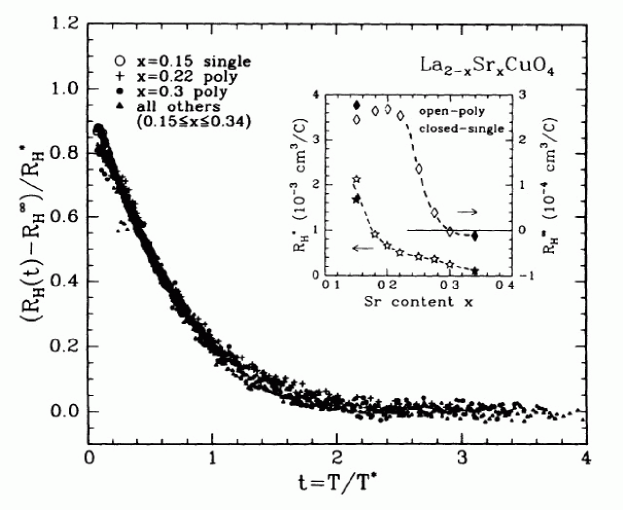
Figure 20: The Hall coefficient ($R_{H}$) for La_2-xSr_xCuO₄ with $0\geq x\geq 0.34$ plotted rescaled as $[R_{H}(t)-R_{H}^{\infty}(x)]/R_{H}^{*}$ vs $t=T/T^{*}$. Inset: the parameters $R_{H}^{\infty}$ and $R_{H}^{*}$ vs Sr composition $x$. The temperature $T^{*}$ agrees with $T^{m}$ obtained from the maximum in the bulk spin susceptibility. Reproduced with permission from [20]

The Hall data for YBa₂Cu₃O_7-y from Ito et al.[19] and Carrington et al.[21] is analyzed in Wuyts et al.[13], who find the following scaling forms (Figs. 21, 22) for the Hall angle, $\theta_{H}(T)$, and the number, $n_{H}(T)$, lead to excellent data collapse:

$$cot(\theta_{H}(T))=cot(\theta_{H}(T^{m}))\frac{T^{2}}{(T^{m})^{2}}\,$$ (37)

$$n_{H}(T)=n_{H}(T^{m})\frac{T}{T^{m}}\,$$ (38)

Wuyts et al.[13] extended the $T$-linear scaling of resistivity near optimal doping to the underdoped regime. Their analysis of Ito et al.’s[19] resistivity data for the YBa₂Cu₃O_7-y family shows that for temperatures $T$ above $T^{m}(x)$ the resistivity is universal and linear (Fig. 23) , and is similar to the optimally doped samples:

$$\rho(T)=\rho(T^{m})\frac{T}{T^{m}}\,$$ (39)

The doping dependence of $T^{m}(x)$ inferred from these scaling forms for the transport coefficients is consistent with its direct magnetic measurements.

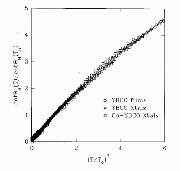
Figure 21: Cotangent of the Hall angle $\cot\theta_{H}$ divided by $\cot\theta_{H}(T_{0})$ vs square of reduced temperature $(T/T_{0})^{2}$ for 15 sets of thin film data together with reported data for oxygen-deficient and Co-doped YBCO single crystals. $T_{0}(x)$ agrees with the temperature obtained by rescaling $Y$ Knight shift. Reproduced with permission from [13].

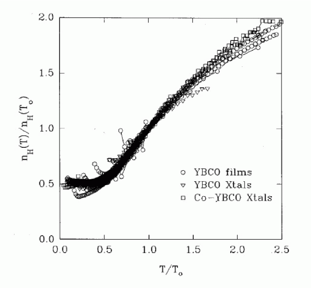
Figure 22: Hall number $n_{H}$ divided by $n_{H}(T_{0})$ vs reduced temperature $T/T_{0}$ for 15 sets of thin film data together with reported data for oxygen-deficient and Co-doped YBCO single crystals. $T_{0}(x)$ agrees with the temperature obtained by rescaling $Y$ Knight shift. Reproduced with permission from [13].

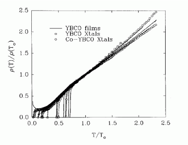
Figure 23: Scaled in-plane resistivity $\rho/\rho(T_{0})$ vs scaled temperature $T/T_{0}$ for 15 sets of thin film data together with reported data for oxygen-deficient and Co-doped YBCO single crystals. $T_{0}(x)$ agrees with the temperature obtained by rescaling $Y$ Knight shift. Reproduced with permission from [13].

Levin and Quader analyzed scaling of the Hall and transport[83, 84] data based on the two-band model Eq.(7) with degenerate ($\xi$) and nondegenerate ($\eta$) carriers. They found that the $T^{2}$ dependence of the cotangent of the Hall angle and the deviations from it can be fit to their model if two lifetimes are introduced for two different bands, $\tau_{\xi}\propto T^{-1}$ and $\tau_{\eta}\propto T^{-2}$. Their two-band model predicts three-parameter scaling for the planar resistivity in the form:

$$\rho=\frac{A(x)T}{\alpha(x)+\Phi(W(x)/T)},$$ (40)

where $W(x)=\Gamma(x-x_{0})$ is the energy scale analogous to $T^{*}$.

A more recent alternative analysis[22] of the high-temperature Hall data[85, 86, 87] for the underdoped La_2-xSr_xCuO₄ family has its basis on the idea of phase separation. It indicates that the Hall data can be understood if one assumes an activated form for the carrier concentration,

$$n_{Hall}=n_{0}(x)+n_{1}(x)\exp{(-\Delta(x)/k_{B}T)},$$ (41)

with a doping-dependent $n_{0}(x)$ that stays linear in $x$ up to $x\simeq 0.12$, above which strong deviations from linearity are observed. The behavior of $\Delta(x)$ was found to be consistent with that measured in photoemission experiments. According to Ref.[22], there is crossover behavior when the number of activated carriers becomes approximately equal to the number of doped carriers $n_{0}(x)$; this occurs at a temperature

$$T^{*}(x)\simeq T_{0}(x)=-\frac{\Delta(x)}{\ln{x}}\,,$$ (42)

that is consistent with characteristic temperatures inferred from other measurements. At a proposed candidate QCP, $x\simeq 0.2$, the energy gap for activated carriers, $\Delta(x)$, goes to zero[22].

2.8 Penetration depth measurements

One of the earliest universal relations that emerged in the high-$T_{c}$ field is the linear Uemura relation[88] between the superfluid density $\rho_{S}$, provided by penetration depth measurements, and the superconducting temperature, $T_{c}$, valid in the underdoped regime. This relation provides an important constraint on the number of electrons that become superconducting. Recently[89] it has been shown (Fig. 24) that a modified Uemura scaling relation,

$$\rho_{S}=120\sigma_{dc}T_{c},$$ (43)

holds for all cuprate superconductors.

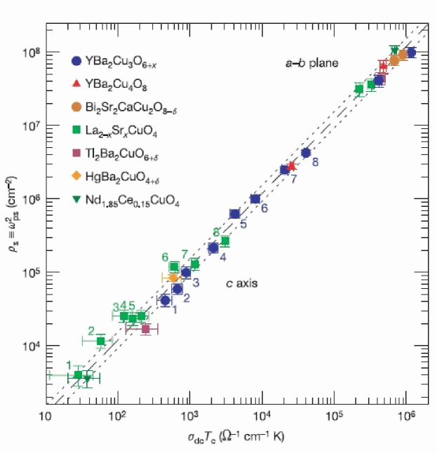
Figure 24: Plot of the superfluid density ($\rho_{S}$) versus the product of d.c. conductivity ($\sigma_{dc}$) and the superconducting transition temperature ($T_{c}$) for various cuprate superconductors. $\sigma_{dc}$ is measured just above the transition. Within error, all of the data fall on the same universal (dashed) line with slope of unity, defined by Eq.(43); the dotted lines are from $\rho_{S}=(120\pm 25)\sigma_{dc}T_{c}.$ Reproduced with permission from [89].

2.9 Angle-resolved photoemission spectroscopy

Enormous progress in resolution has been made in angle-resolved photoemission spectroscopy (ARPES) experiments in the past decade so that ARPES has now emerged as one of the best experimental probes of the cuprates[90]. One of the most important contributions of ARPES was the detection of the anisotropic normal state gap in the fermionic spectrum, first by Marshall et al.[91], Loeser et al.[92], and then by Ding et al.[93] in Bi₂Sr₂CaCu₂O_8+δ.

By examining their data, Marshall et al. concluded that the normal state gap has two energy scales. They identified the low energy scale gap ($\sim 20-30meV$) by the location of the leading-edge midpoint. This is a clear gap in the fermionic spectrum that has a $d$-wave-like momentum dependence, with gapless Fermi surface arcs near the nodal regions. The high energy scale ($\sim 100-200meV$) gap appears as a broad incoherent feature in the spectrum near the $(\pi,0)$ point, where the low-energy spectral weight is strongly suppressed. The low energy leading-edge gap first appears below $T^{*}(x)$, a temperature that has the same doping dependence as $T^{m}(x)\sim J_{eff}(x)$ observed in other measurements. However, $T^{*}$ inferred from ARPES measurements[90, 28] in Bi₂Sr₂CaCu₂O_8+δ turns out to be significantly lower than $T^{m}$, $T^{*}(x)\simeq T^{m}(x)/3\simeq J_{eff}(x)/3$. Both the measured magnitude and the $\bm{k}$-dependence of the normal state leading edge gap are very similar to that of the d-wave gap in the superconducting state; the normal state gap smoothly evolves into a superconducting gap below $T_{c}$. The doping dependence of the normal state d-wave-like gap amplitude $\Delta(x)$ tracks that of $T^{*}(x)$[90, 28].

The ratio of $T^{*}(x)$ and $T^{m}(x)$ varies for different families of materials. Detailed ARPES investigations of the La_2-xSr_xCuO₄[94, 95] and other families of cuprate superconductors[90] find the same general form of the spectrum and the same linear doping dependence of the energy gap amplitude $\Delta(x)\propto T^{m}(x)$ as that found in the Bi₂Sr₂CaCu₂O_8+δ family of materials. Following these and other ARPES results, Damascelli et al.[90] suggest that the value of $T^{*}(x)$ and $\Delta(x)$ is determined by the maximum value of $T_{c}$ for a given material, $T_{c}^{max}$, rather than exchange coupling $J$:

$$\Delta(x)\propto T^{*}(x)\propto T_{c}^{max}$$ (44)

The high energy incoherent feature of the ARPES spectra also has a d-wave like dispersion[28]. It is often claimed to be a remnant of the antiferromagnetic insulator[90], since it exhibits the same dispersion[28] along the $(0,0)$-$(\pi,0)$ and $(\pi,\pi)$ - $(\pi,0)$ directions, which are only equivalent in the reduced antiferromagnetic Brillouin zone, and is similar to the ARPES spectra observed in undoped antiferromagnetic insulators.

The fact that the normal state gap closes non-uniformly in momentum space with increased temperature or doping has been well established for some time[90]. Recently Kanigel et al.[6] investigated the temperature- and doping- dependence of the low energy normal state gap in several samples of Bi2212 and discovered a remarkable scaling relation: the anisotropy of the normal state gap and the length of the gapless Fermi arcs near the nodal region for these different samples depend only on a single parameter, a reduced temperature $t=T/T^{*}(x)$ (Fig. 25). Kanigel et al. also found that the length of gapless Fermi arcs near the nodes above the superconducting temperature $T_{c}$ is linear in $t$, while below $T_{c}$ the Fermi arcs develop the usual d-wave superconducting gap with point nodes.

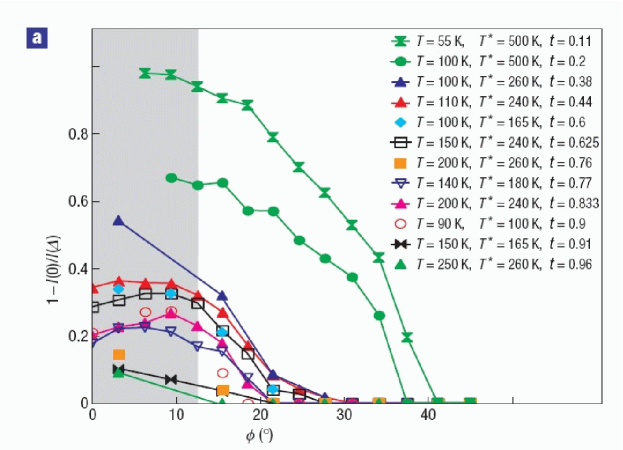
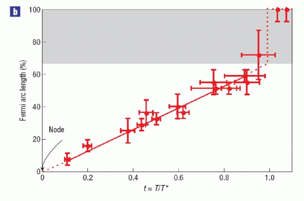
Figure 25: (a) Loss of low-energy spectral weight $L(\varphi)=[1-I(0,\varphi)/I(\Delta,\varphi)]$, where $I(\Delta,\varphi)$ is the symmetrized intensity at the gap energy at the Fermi point labeled by angle $\varphi$, and $I(0,\varphi)$ is that at the Fermi energy at the same point. Different symbols correspond to different $t$. The gray area represents the straight section of the Fermi surface (b) Variation of the arc length with respect to reduced temperature $t=T/T^{*}$. On the y axis, 0 % is the node and 100 % is the antinode. Reproduced with permission from [6].

Is the superconducting gap that develops at $T_{c}$ in the nodal Fermi arc region the same as the normal state gap, or is it a different gap? Recently Millis[96] argued that this important question has not been resolved for years, since different experimental studies yield conflicting results. An experimental observation of two different gaps in the underdoped regime will confirm that the normal state gap in the underdoped cuprates is driven by a different, competing nonsuperconducting order, not pairing fluctuations[97]. Since the superconducting gap in the nodal region is extremely small, answering this question in ARPES requires a very high resolution study. So far ARPES studies have proved to be conflicting as well[96]. For example, a recent leading edge gap ARPES study of Tanaka et al.[98] on three different samples of Bi2212 found that the superconducting gap in the nodal arc region had a doping dependence different from that of $T^{*}(x)$, and scaled with $T_{c}(x)$ instead. On the other hand, Valla et al.[99] reported that the energy gap in a non-superconducting sample of La_1.875Ba${}_{0}.125$CuO₄, where the superconducting order is suppressed by charge ordering, has essentially the same simple d-wave form and magnitude as in the superconducting sample at higher doping concentration, thus yielding crucial support to the single gap scenario.

2.10 STM Experiments

All STM studies find strong nanoscale inhomogeneity, in which gap magnitudes are observed to vary strongly on the nanometer length scale, while the recent STM measurements of Alldredge et al.[7], Gomez et al.[8], and Boyer et al.[100] provide detailed evidence on gap formation in the underdoped 2212 and 2201 families of cuprates.

According to Gomez[8], in the overdoped regime locally there is only one gap that has a d-wave symmetry. The distribution of the energy gaps is, nevertheless, very inhomogeneous, indicating the presence of disorder. As the temperature is raised above $T_{c}$, the total spatial area of ungapped regions increases until the whole sample becomes ungapped. The local temperature $T_{p}$ at which the normal state gap first appears varies strongly in space. Nevertheless, the ratio of the local gap maximum $\Delta_{max}$ in $\bm{k}$-space to the local ordering temperature $T_{p}$ turns out to be universal for different spatial regions and very large[8], $2\Delta/k_{B}T_{p}=7.7$, much greater than the d-wave BCS limit of $4.3$, indicating strong coupling.

In the underdoped regime, Gomez et al. first see the spatially inhomogeneous formation of the local gaps below $T^{*}$, defined as the temperature at which 90 % of the sample becomes gapped. Below $T_{c}$, Gomez et al. observe the formation of a smaller kink inside the larger local gap, corresponding to the onset of superconductivity. They conclude that in the underdoped regime there are two energy scales, with the lower energy scale corresponding to the onset of phase coherence. Boyer et al.[100] adopted a different approach in their analysis of their STM measurements on an overdoped sample, a member of Bi2201 family, (Bi_1-yPb_y)₂Sr₂CuO_6+x (T${}_{c}=15K$). Since inhomogeneity is unaffected by the onset of superconductivity at $T_{c}$, Boyer et al. look for the signature of superconductivity, the emergence of the subgap kink at T_c, by removing the effective background of the high-temperature STM spectra, which is largely unaffected by the onset of superconductivity, from the low-temperature spectra. As a result of this subtraction, they find a second, homogeneous superconducting gap, $\Delta_{small}=6.7\pm 1.6meV$ that forms at $T_{c}=15K$. Their analysis thus strongly suggests that the subgap kink at $T_{c}$, also seen by Gomez et al., rather than being an onset of phase coherence, corresponds to the opening of superconducting gap at $T_{c}$.

Alldredge et al.[7] have studied the tunneling density of states in momentum space. Their analysis indicates that there is only one gap in the underdoped materials. Alldredge et al. find that a large effective anisotropic scattering rate $\Gamma(\bm{k})\propto|\Delta(\bm{x}|$ is needed to fit their data in the underdoped regime. Their effective scattering rate becomes non-zero at $x\leq 0.22$, and increases approximately linearly with decreased doping, similarly to the normal state energy gap. Thus, they conclude, they have effectively two kinds of quasiparticles in the underdoped regime: quasiparticles near the $(\pi,0)$ antinodes in momentum space that are incoherent and almost localized, and coherent quasiparticles in the nodal region.

3 A two-fluid analysis of experimental data

The observations of data collapse reviewed in the previous section provide two very important constraints on any theory of the underdoped cuprate superconductors. They indicate the presence of two distinct fluids whose composition might be expected to vary with doping: a spin liquid containing localized Cu spins with a doping-dependent effective interaction and a Fermi liquid whose transport properties differ markedly from those of a Landau Fermi liquid. In this section we develop a two-fluid framework for analyzing these experiments and use it to extract their consequences. We present as well the details of our earlier analysis[3] of the magnetic measurements of two fluid behavior.

3.1 Two-Fluid Description

Our approach is inspired by the success of the two-fluid phenomenology developed for the 1-1-5 family of heavy electron materials[101, 102]. For these and other heavy electron materials containing a Kondo lattice of localized $f$-electrons coupled to a conduction band, a two-fluid phenomenological model of the hybridization of the $f$ electron localized spins with those in the conduction band describes very well the emergence of a hybridized non-Landau heavy electron Fermi liquid that coexists with unhybridized local f-electrons and conduction electrons. The emergence of two components in the bulk spin susceptibility and the Knight shift in the cuprates can be understood by writing the total spin of the system as a sum of the localized $d$-electron and $p$-hole spins,

$$\bm{S}_{tot}=\sum_{i}\bm{S}^{d}(\bm{r}_{i})+\sum_{j}\bm{S}^{p}(\bm{r}_{j}),$$ (45)

where $\bm{r}_{i}$ are the positions of copper $d$-electrons, $\bm{r}_{j}$ the positions of oxygen p-holes. Quite generally, the coupling between these spins gives rise to three contributions to spin susceptibility[102],

$$\chi=\chi_{dd}+2\chi_{dp}+\chi_{pp},$$ (46)

where $\chi_{dd}$ represents the contribution from the localized Cu spins, $\chi_{pp}$ represents the part of the oxygen $p$-band that is not hybridized, while $\chi_{dp}$ corresponds to the magnetic response of the hybridized quasiparticles with a large Fermi surface:

$$\chi_{dd} = \frac{1}{N}\,\sum_{i,i^{\prime}}\langle\bm{S}^{d}(\bm{r}_{i})\bm{S}^{d}(\bm{r}_{i^{\prime}})\rangle$$ (47)

$$\chi_{dp} = \frac{1}{N}\,\sum_{i,j}\langle\bm{S}^{d}(\bm{r}_{i})\bm{S}^{p}(\bm{r}_{j})\rangle$$ (48)

$$\chi_{pp} = \frac{1}{N}\,\sum_{j,j^{\prime}}\langle\bm{S}^{p}(\bm{r}_{j})\bm{S}^{p}(\bm{r}_{j^{\prime}}).\rangle$$ (49)

The Fermi liquid contribution to spin susceptibility thus arises from $\chi_{pd}$ and $\chi_{pp}$. Only the position of oxygen holes is important for the above decomposition; whether or not they form a single hybridized band is irrelevant. The three parts are present in an explicit two-band model of Walstedt et al.[36] that produces correct expressions for the relaxation rates in terms of $\chi_{pp}$, $\chi_{pd}$, and $\chi_{dd}$. It differs from the standard Mila-Rice-Shastry/MMP[32, 40] ionic model that assumes a single spin degree of freedom residing on the copper site, so that $\chi_{pd}=\chi_{pp}\equiv 0$ and the hybridized $pd$ band description of Millis and Monien[103], in which although $\chi_{pp}$, $\chi_{pd}$, and $\chi_{dd}$ are taken to be non-zero, all three components are assumed to track the spin susceptibility of a single hybridized $pd$ band.

The scaling results of the previous section tell us that $\chi_{dd}$ must maintain its local character throughout much of the phase diagram, for how else could the bulk susceptibility and the low frequency magnetic response map onto the 2D Heisenberg model? To describe this we therefore write:

$$\chi_{dd}=f(x)\chi_{SL}(\bm{q},\omega)$$ (50)

where $f(x)$ is the fraction of the $dd$ (and the total) response function that retains its local spin character, while the remaining portion of the spin-spin response function describes the response of a (non-Landau) Fermi liquid with the large Fermi surface that results from hybridization:

$$2\chi_{dp}+\chi_{pp}=[1-f(x)]\chi_{FL}(\bm{q},\omega).$$ (51)

We thus arrive at the two fluid description,

$$\chi(\bm{q},\omega)=f(x)\chi_{SL}(\bm{q},\omega)+[1-f(x)]\chi_{FL}(\bm{q},\omega),$$ (52)

that we will use in our subsequent analysis to extract from experiment the doping dependence of both $\chi_{SL}$ and $f(x)$.

The spin liquid contribution completely determines the low frequency dynamic magnetic spin susceptibility measured by NMR on copper nuclei. It corresponds to the scaled spin response of the 2D Heisenberg model for localized copper spins, which in the low frequency limit can be written in a general phenomenological form proposed by Millis, Monien, and Pines[40], modified to include the possibility of propagating spin wave excitations [104]:

$$\chi_{SL}(\bm{q},\omega)=\frac{\alpha\xi^{2}}{1+\xi^{2}(\bm{q}-\bm{Q})^{2}-i\frac{\omega}{\omega_{SF}}\,-\frac{\omega^{2}}{\Delta_{SL}^{2}}\,}\,,$$ (53)

where $\Delta_{SL}=c/\xi$ is the gap in spin excitation spectrum. We note that in general damping in the Heisenberg model is caused by the spin wave scattering, so that the relaxational frequency, $\omega_{SF}$, must be, in general, frequency-dependent in the underdoped cuprates. We further note that if one assumes Heisenberg model scaling, then, from dimensional arguments, $\alpha(x)=\chi_{\bm{Q}}\xi^{-2}$ is proportional to $1/T^{m}(x)$.

The Walstedt et al. generalization of the Mila-Rice-Shastry hyperfine Hamiltonian for Cu site can be written as:

$${}^{63}H_{hyp}=\sum_{\rho}\left\{{}^{63}I_{\rho}[A_{\rho}\bm{S}_{\rho}^{d}+B\sum_{i}\bm{S}_{\rho}^{d}(\bm{r}_{i})]+^{63}I_{\rho}D\sum_{j}\bm{S}^{p}_{\rho}(\bm{r}_{j})\right\}$$ (54)

Here $i$ corresponds to the nearest neighbor Cu sites, $\rho=a,b,c$ while $D$ is a new transferred hyperfine constant for the spins sitting on oxygen. The sum index $j$ goes over the oxygen sites neighboring the copper site. Similarly, one can write the hyperfine Hamiltonian for the oxygen nuclei:

$${}^{17}H_{hyp}=\sum_{\rho}\left\{{}^{17}I_{\rho}C\sum_{i}\bm{S}^{d}_{\rho}(\bm{r}_{i})+^{17}I_{\rho}E_{\rho}\bm{S}^{p}_{\rho}\right\}$$ (55)

Here $C$ is the transferred hyperfine coupling constant for localized Cu spins and $E_{\rho}$ is the contact hyperfine interaction for the oxygen nucleus; the sum index $i$ goes over the NN copper sites. Making use of

$$\mu_{B}\langle S^{p}(\bm{r})\rangle = (\chi_{pd}+\chi_{pp})\bm{B}_{ext}$$ (56)

$$\mu_{B}\langle S^{d}(\bm{r})\rangle = (\chi_{pd}+\chi_{dd})\bm{B}_{ext},$$ (57)

where $\bm{B}_{ext}$ is the strength of the external magnetic field and $\mu_{B}$ is the electron magnetic moment, we get, from the above Hamiltonians:

$${}^{63}K_{\rho} = {}^{63}K_{0,\rho}+\frac{A_{\rho}+4B}{{}^{63}\gamma_{n}\mu_{B}^{2}\hbar^{2}}\,(\chi_{dd}+\chi_{pd})+\frac{4D}{{}^{63}\gamma_{n}\mu_{B}^{2}\hbar^{2}}\,(\chi_{pd}+\chi_{pp})$$ (58)

$${}^{17}K_{\rho} = {}^{17}K_{0,\rho}+\frac{2C}{{}^{17}\gamma_{n}\mu_{B}^{2}\hbar^{2}}\,(\chi_{dd}+\chi_{pd})+\frac{E_{\rho}}{{}^{17}\gamma_{n}\mu_{B}^{2}\hbar^{2}}\,(\chi_{pd}+\chi_{pp}).$$ (59)

Here $\gamma_{n}$ are the corresponding nuclear gyromagnetic ratios. On introducing the dynamic spin susceptibilities,

$$\chi_{\mu\nu}(\bm{q},\omega)=\langle\langle S^{\rho}_{\mu}(\bm{q})S^{\rho}_{\nu}(-\bm{q})\rangle\rangle_{\omega},$$ (60)

where $\mu,\nu=p,d$, we obtain the Walstedt et al. expression for relaxation rates:

$$\frac{1}{{}^{\alpha}T_{1\gamma}T}\,=\frac{k_{B}}{2\mu_{B}^{2}\hbar^{2}}\,\lim_{\omega\rightarrow 0}\sum_{\bm{q},\mu,\nu=p,d}\,^{\alpha}F_{\gamma,\mu\nu}(\bm{q})\frac{Im\chi_{\mu\nu}(\bm{q},\omega)}{\omega}\,,$$ (61)

where $\gamma$ is the direction of magnetic field, $\alpha$ is the nuclear site. For $\chi_{dd}$ one gets the usual MMP form factors:

$${}^{63}F_{\parallel,dd}(\bm{q})=(A_{\perp}+2B(\cos(q_{x}a)+\cos(q_{y}a))^{2},$$ (62)

$${}^{63}F_{\perp,dd}(\bm{q})=\frac{1}{2}\,^{63}F_{\parallel,dd}(\bm{q})+\frac{1}{2}\,(A_{\parallel}+2B(\cos{q_{x}a}+\cos{q_{y}a}))^{2},$$ (63)

$${}^{17}F_{\gamma,dd}(\bm{q})=2C^{2}(1+\cos(q_{x}a)).$$ (64)

The form factors for the mixed p-d contribution are:

$${}^{63}F_{\parallel,pd}(\bm{q})=^{63}F_{\parallel,dp}(\bm{q})$$

$$=2D(\cos{(q_{x}a/2)}+\cos{(q_{y}a/2)})(A_{\perp}+2B(\cos{q_{x}a}+\cos{q_{y}a})),$$ (65)

$${}^{63}F_{\perp,pd}(\bm{q})=^{63}F_{\perp,dp}(\bm{q})$$

$$=D(\cos{(q_{x}a/2)}+\cos{(q_{y}a/2)})(A_{\perp}+A_{\parallel}+4B(\cos{q_{x}a}+\cos{q_{y}a})),$$ (66)

$${}^{17}F_{\parallel,pd}(\bm{q})=^{17}F_{\parallel,dp}(\bm{q})=2CE_{\perp}\cos{(q_{x}a/2)},$$ (67)

$${}^{17}F_{\perp,pd}(\bm{q})=^{17}F_{\perp,dp}(\bm{q})=C(E_{\perp}+E_{\parallel})\cos{(q_{x}a/2)}.$$ (68)

Finally, for the p-p part of spin susceptibility:

$${}^{63}F_{\gamma,pp}(\bm{q})=4D^{2}(\cos{(q_{x}a/2)}+\cos{(q_{y}a/2)})^{2}$$ (69)

$${}^{17}F_{\parallel,pp}(\bm{q})=E_{\perp}^{2}$$ (70)

$${}^{17}F_{\perp,pp}(\bm{q})=\frac{1}{2}\,E_{\perp}^{2}+\frac{1}{2}\,E_{\parallel}^{2}$$ (71)

Apart from ${}^{17}F_{pp}(\bm{q})$, the form factors for the p-d and p-p contributions vanish at $\bm{Q}=(\pi/a,\pi/a)$:

$${}^{17}F_{pd}(\bm{Q})=^{63}F_{pd}(\bm{Q})=^{63}F_{pp}(\bm{Q})=0.$$ (72)

In what follows we focus on the behavior of planar dynamic and static magnetic response and the thermodynamic behavior, as measured by the inelastic neutron scattering, NMR, heat capacity and bulk spin susceptibility.

3.2 Scaling for bulk spin susceptibility and Knight shift

We now apply our two-fluid description to an analysis of the bulk spin susceptibility and Knight shift measurements in La_2-xSr_xCuO₄ and YBa₂Cu₃O_6+x families of cuprate superconductors. For the static susceptibility, the two components in Eq.(52) can be written in the following form:

$$\chi(T)=f(x)\chi_{SL}(T/T^{m}(x))+(1-f(x))\chi_{FL}+\chi_{0},$$ (73)

where

$$\chi_{0}=\chi_{VV}+\chi_{core}.$$ (74)

Here $\chi_{VV}$ and $\chi_{core}$ are temperature- and doping-independent Van Vleck and core contributions. $\chi_{0}$ is usually taken to be diamagnetic, due to a large core contribution[2]. As noted earlier, $\chi_{SL}$ follows very well the calculated[5] bulk spin susceptibility for the Heisenberg model with a doping-dependent exchange constant $J_{eff}(x)\sim T^{m}(x)$. Thus, the spin liquid contribution to static magnetic response can be written as

$$f(x)\chi_{SL}(T/T^{m}(x))=\chi^{m}\tilde{\chi}(T/T^{m}(x)),$$ (75)

where $\chi^{m}$ is the maximum value of the spin liquid susceptibility and $\tilde{\chi}(T/T^{m}(x))$ is a universal function of $T/T^{m}$.

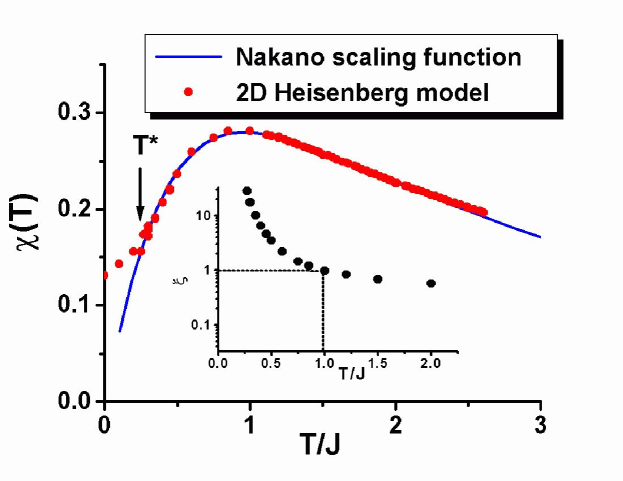
Figure 26: Comparison of the scaling curve for bulk spin susceptibility data in underdoped metallic La_2-xSr_xCuO₄ from Nakano et al.[11] to the Heisenberg model numerical calculations of Makivić and Ding[5]. The maximum for spin susceptibility is reached at $T^{m}\simeq 0.93J$. Deviations from the Heisenberg model results are observed for $T<T^{*}\simeq T^{m}/3$. The inset shows the numerical results for the correlation length[5], that demonstrate that $\xi\simeq 1$ at temperature $T\simeq T^{m}$.

A comparison of the universal data collapse curve for the bulk spin susceptibility in La_2-xSr_xCuO₄ family found by Nakano et al.[11] to the Heisenberg model calculations[5] is shown in Fig.26. We see that the universal function of Nakanoet al. deviates significantly from the 2D Heisenberg model results at low temperatures, $T<T^{*}\simeq T^{m}/3$.

As noted earlier, the scaling analysis of Nakano et al.[11] differs from that of Johnston[2], because it includes at lower doping levels a Curie term $C/T$, and a linear term $B(T-T_{a})$ in the static spin response. While the inclusion of these terms may be justified, it introduces a number of new parameters that are, in a sense, unnecessary since the universal curve in the insulating compound must agree with the 2D Heisenberg model results. We therefore omit these terms in our analysis, and we assume, in agreement with recent photoemission studies[6], that the Fermi liquid contribution, $\chi_{FL}(T,x)$, is temperature-independent above $T^{*}$, but could, for the 1-2-3 materials become temperature-dependent below the temperature, $T^{*}$, at which a gap starts to form in the quasiparticle energy spectrum, leading to the formation of the Fermi arcs.

To determine the doping dependence of the parameters in Eq.(73), we analyzed the bulk spin susceptibility data[11] for metallic underdoped La_2-xSr_xCuO₄. With a constant contribution $\chi_{0}+\chi_{FL}(x)$ subtracted, we find, in agreement with the earlier results[2, 12, 11], the data collapse to the 2D Heisenberg model curve, shown in Fig. 27, where we see that the data collapse continues below the temperature $\sim T^{m}/3$ at which one no longer finds agreement with the Heisenberg model.

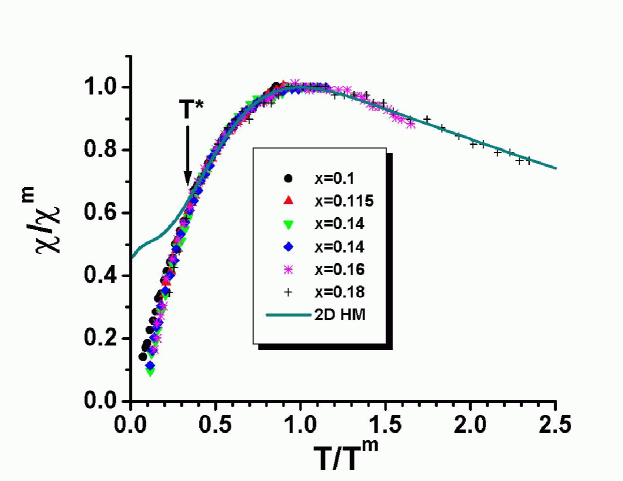
Figure 27: Comparison of the bulk spin susceptibility data in underdoped metallic La_2-xSr_xCuO₄ from Nakano et al.[11] to the Heisenberg model numerical calculations of Makivić and Ding[5]. The maximum for spin susceptibility is reached at $T^{m}\simeq 0.93J$. While the data collapse remains reasonably good even at low temperatures, large deviations from 2D Heisenberg model prediction are observed for $T<T^{m}/3$.

A similar scaling analysis for the ${}^{63}Cu$ Knight shift data in 1-2-3 materials is shown in Fig.28.

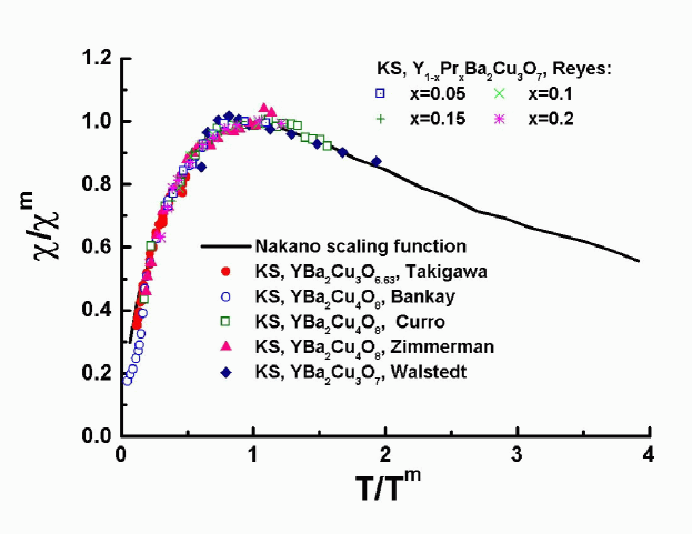
Figure 28: Scaling for the ${}^{63}Cu$ Knight shift[37, 33, 105, 106, 107, 108] in YBa₂Cu₃O_6+x, compared to the scaling function obtained by Nakano et al.[11] for the bulk spin susceptibility in La_2-xSr_xCuO₄. $T^{m}$ is the temperature at which the Knight shift has a maximum.

The doping dependence of $T^{m}(x)\simeq 0.93J_{eff}(x)$ that follows from the analysis of the bulk susceptibility and Knight shift data, is shown in Fig. 29 for both La_2-xSr_xCuO₄ and YBa₂Cu₃O_6+x families. $T^{m}(x)$ falls linearly with increased doping $x$ for both materials. For La_2-xSr_xCuO₄, and doping levels less than $0.18$,

$$T^{m}(x)=1218K(1-4.45x).$$ (76)

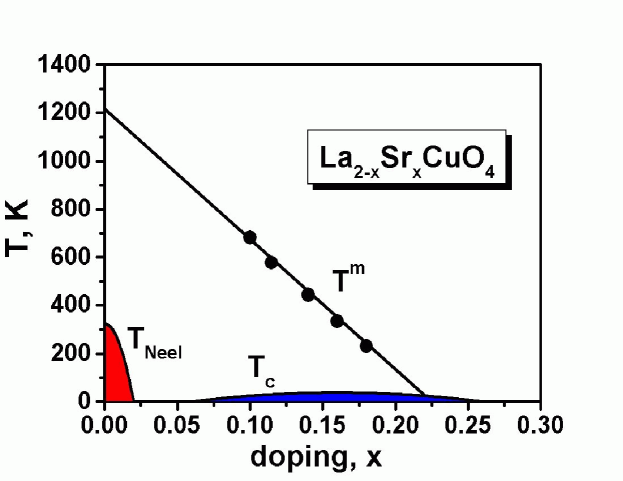
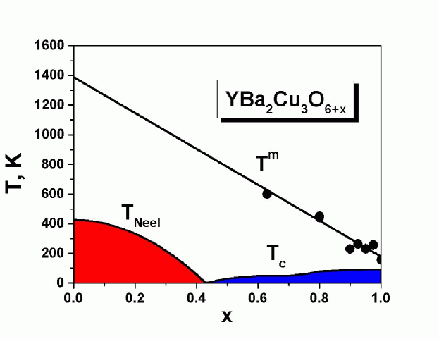
Figure 29: (a) The temperature $T^{m}(x)$ that follows from our analysis of the Nakano et al.[11] bulk spin susceptibility data for La_2-xSr_xCuO₄, and (b) the Knight shift data for YBa₂Cu₃O_6+x

Our analysis of the bulk susceptibility data in La_2-xSr_xCuO₄ also enables us to extract the doping dependence for the Fermi liquid and spin liquid components. The results for $\chi^{m}(x)$ and $\chi_{FL}(x)$ given by Eqs.(75),(73) are shown in Fig.30.

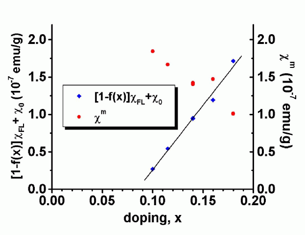
Figure 30: $\chi^{m}(x)$ and $\chi_{FL}(x)$, from our analysis of the bulk susceptibility measurements in La_2-xSr_xCuO₄. Here $\chi_{FL}(x)$ here also includes a diamagnetic constant, $\chi_{0}$, hence the non-zero offset.

The doping dependence for the fractional occupation, $f(x)$, of the spin liquid state can be determined from $T^{m}(x)$ and $\chi^{m}(x)$. The dimension of $\chi$ is $1/energy$. Thus, since the universal curve for $T>T^{*}$ coincides with the numerical calculation for the 2D Heisenberg antiferromagnet with $T^{m}\simeq 0.93J_{eff}$, we can write:

$$\chi_{SL}(T/T^{m}(x))\propto\frac{1}{T^{m}(x)}\,\tilde{\chi}(T/T^{m}(x)),$$ (77)

where $\tilde{\chi}(T/T^{m}(x))$ is a universal function for the Heisenberg antiferromagnet. Using Eqs(77) and (75), the doping dependence of $f(x)$ is then determined by the product $\chi^{m}(x)T^{m}(x)$:

$$f(x)=\frac{\chi^{m}(x)T^{m}(x)}{\chi^{m}(x=0)T^{m}(x=0)}\,$$ (78)

From our data analysis, we find that for the doping levels available for our analysis, $f(x)$ also decreases linearly with $x$,

$$f(x)=1-4.977x,$$ (79)

as shown in Fig. 31, so that $T^{m}(x)$ and $f(x)$ roughly track each other.

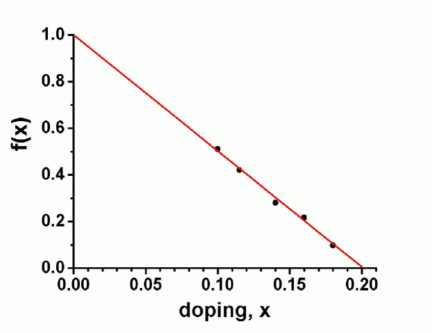
Figure 31: The spin liquid fraction $f(x)$, from our analysis of the bulk susceptibility measurements in La_2-xSr_xCuO₄[11].

Fig. 30 also shows the doping dependence for the Fermi liquid component, $\chi_{FL}(x)=(1-f(x))\chi_{FL}+\chi_{0}$. We find that the Fermi liquid component increases linearly with doping in the metallic regime, in agreement with Eq.(73). The offset for this linear dependence is due to the presence of $\chi_{0}$, which is diamagnetic [2]. Since $f(x)$ also decreases linearly with $x$, we conclude that $\chi_{FL}$ in Eq.(73) has only mild, if any, doping-dependence.

3.3 Knight shift data

We now examine the Knight shift data in more detail. As noted in Section 2, most early Knight shift experiments on different nuclei found the same temperature-dependent contribution to spin susceptibility[33, 34, 109], although some deviations from this universality (within error bars) can be seen on the universal plot below the superconducting temperature $T_{c}$[33, 34]. The linear $K-\chi$ and $K-K$ plots above $T_{c}$, observed in many early Knight shift experiments, then provide a measurement of the hyperfine couplings to single copper spin. These measurements had been regarded as a key proof of an effective one-component model. However, the Cu Knight shift measurements on the 1-2-4 material by Suter et al.[38] and the recent apical oxygen Knight shift measurements in La_1.85Sr_0.15CuO₄ by Haase et al.[39], tell a different story, and we consider these now.

The Knight shift measurements of Suter et al. were done for an external magnetic field in the c direction, where, because of the well-known accidental cancellation[40] of the $\chi_{dd}$ form factor, $A_{\parallel}+4B$, in Eq.(58), within the single-component approximation, the Knight shift for fields along the c-axis would be of purely orbital origin. Within the two-fluid description, we see from Eq.(58) that one can, in addition, probe Fermi liquid behavior through an isotropic transferred hyperfine interaction $D$ that arises from the hybridization of planar oxygen p-orbitals and copper s-orbitals. So to the extent that the Fermi liquid susceptibility becomes temperature dependent as a result of a quasiparticle gap opening up at $T^{*}$,one would expect to see this in ${}^{63}K_{\parallel}$. As may be seen in Fig. 32, where we have extracted the behavior of $\chi_{pp}+\chi_{pd}$ as a function of T from their Knight shift measurements, this is just what was found by Suter et al.[38]. The anomalous Fermi liquid behavior begins at a temperature, $T^{*}\sim 180K\sim 0.4T^{m}$ for YBa₂Cu₃O₈, an onset temperature that is consistent with the onset of Fermi arc behavior at a comparable value of $T^{*}$ seen in the ARPES measurements on underdoped 2212 materials.

In their recent re-analysis of the planar ⁶³Cu and ¹⁷O Knight shift experiments on La_1.85Sr_0.15CuO₄ that was accompanied by new apical oxygen Knight shift experimental results, Haase et al.[39] have found convincing experimental evidence for the existence of both a Fermi liquid and a spin liquid component in this material. They show that while all nuclei see the same temperature-dependent spin liquid component, the different nuclei see as well a component that is independent of temperature above the superconducting transition temperature, $T_{c}$, but displays the expected d-wave signature below $T_{c}$, and hence must be associated with a Fermi liquid component, rather than representing an orbital or Van Vleck core term.

Quite importantly, they combine their results in the superconducting state (that include correcting for any Meissner shielding effects) and the normal state for magnetic fields in and perpendicular to the CuO planes with Equations (58) and (59), supplemented by an equivalent expression for the apical oxygen site, to determine all the relevant hyperfine couplings. They show these can be used to determine the strength and temperature dependence in the normal and superconducting states of all three components, $\chi_{dd}$, $\chi_{dp}$, and $\chi_{pp}$. We refer the interested reader to their paper for the details of their findings, which place important constraints on any description of the hybridization of the Cu $d$ electrons with the oxygen $p$ band.

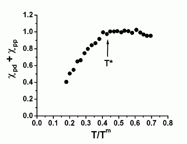
Figure 32: Normalized temperature dependence of $\chi_{pd}$ as a function of $T/T^{m}$, inferred from ${}^{63}K_{c}$ measurements[38] in YBa₂Cu₃O₈.

While further Knight shift measurements under conditions favorable to observing the Fermi liquid component are highly desirable, we believe it is reasonable to conclude that the two-fluid analysis of Knight shift in heavy electron materials[102] extends naturally to high-$T_{c}$ superconductors, with

$$\chi_{dd}=f(x)\chi_{SL},$$ (80)

and

$$\chi_{pp}+2\chi_{pd}=(1-f(x))\chi_{FL}.$$ (81)

Eq. (81) can then be combined with the results of Haase et al., and our previously determined value of $f(x)$, to determine the doping-independent quantity $\chi_{FL}$ for the 2-1-4 materials. The results of this analysis can be checked by extending the Haase et al. analysis to other doping levels.

3.4 ${}^{63}Cu$ NMR Relaxation Rates

In analyzing the NMR relaxation rates, we shall focus on the ${}^{63}Cu$ spin-lattice relaxation rate, ${}^{63}T_{1}$, and the spin-echo-decay time, ${}^{63}T_{2G}$. As discussed in the beginning of the section, there are different components of the spin response. However, due to the large peak of the spin-liquid part at $\bm{Q}=(\pi,\pi)$, and the corresponding non-vanishing form factors for ${}^{63}Cu$ nuclei, the copper relaxation rates primarily probe the low-frequency properties of the spin-liquid contribution that arises from $\chi_{dd}=f(x)\chi_{SL}$ part of the spin susceptibility. In our modification of MMP[40] both $\chi_{pd}$ and $\chi_{pp}$ correspond to the contribution of fermions with a large hybridized Fermi surface, or pieces of such a Fermi surface, in agreement with the Knight shift measurements of Haase et al.[39], and therefore have a negligible effect on copper relaxation rates. An alternative possibility, that we mention only briefly, is that the two components seen in the bulk measurements are a result of microscopic phase separation and formation of dynamic stripes. Surprisingly, while the transition points that we obtain from the two-component analysis of bulk measurements coincide with the well-known region of phase separation in La₂CuO_4+δ[110], the two-component nature is evident in bulk measurements at temperatures well above the phase separation temperature region.

Where these can both be carried out, measurements of ${}^{63}Cu$ spin-lattice relaxation and spin-echo decay rates indicate the presence of two different dynamic scaling regimes that lie above and below $T^{m}$[9]. Above $T^{m}$ one is in a mean-field, $z=2$ scaling regime, in which the relaxational frequency, $\omega_{SF}$ varies as $1/\xi^{2}$; below $T^{m}$ it varies as $1/\xi$ because the spin liquid has entered the $z=1$ dynamic scaling regime[9, 18] expected for the quantum critical (QC) regime of a 2D antiferromagnet. As discussed in Ref.[9], one can describe the spin dynamics using the quantum non-linear sigma model, or spin wave theory[47, 48]. The resulting QC scaling theory[48] for the spin liquid without long-range order gives a linear dependence of the correlation length on temperature,

$$\frac{1}{\xi(T,x)}\,=1.04\frac{T}{c}\,+a(x),$$ (82)

where $c\propto J\sim T^{m}$ is the spin wave velocity, and the offset $a(x)>0$ goes to zero at $x_{c}$, a quantum critical point for the spin liquid that marks the onset of long-range order. A similar linear dependence on $T$ can be expected also for ${}^{63}T_{1}T\propto\omega_{SF}$[9, 18],

$${}^{63}T_{1}T=A(x)+\kappa T^{m}\frac{T}{T^{m}}\,,$$ (83)

with an offset $A(x)$ that measures the distance from the proposed quantum critical point, while $\kappa$ is a universal coefficient.

Quantum critical theory applies in the universal regime, $\xi\gg 1$, thus, well below $T^{m}$. Scaling of the form seen in Eq.(83) is self-evident from the low-temperature ${}^{63}T_{1}$ data on La_2-xSr_xCuO₄ material of Ohsugi et al.[49](Fig.7). When they plot the product ${}^{63}T_{1}T$ vs temperature in the metallic underdoped regime, they find a set of parallel lines for their different doping levels that extend from $T\sim 300K$ down to a low-temperature upturn in ${}^{63}T_{1}T$ that is near $T_{c}$. We plot in Figs.33,34 the scaling behavior for ${}^{63}T_{1}$ in the 2-1-4 and the 1-2-3 materials. The $x$ dependence of the off-set, $A(x)$, of the low-temperature linear behavior in ${}^{63}T_{1}T$ points to a critical point in the spin liquid at $x=0.05$, separating long range order from short range order, a result that was also suggested earlier in an analysis of the high-temperature ${}^{63}T_{1}$ data[18].

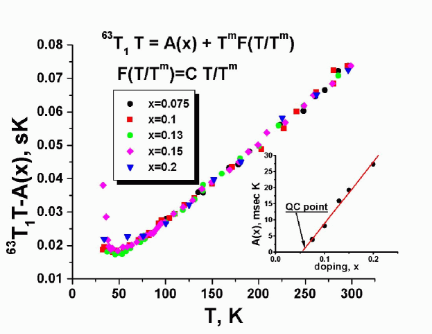
Figure 33: Scaling for the NMR relaxation rate $T_{1}$ in La_2-xCuO₄[49] The offset $A(x)$ shown in the inset depends linearly on $x$, and points to a QCP in the spin liquid.

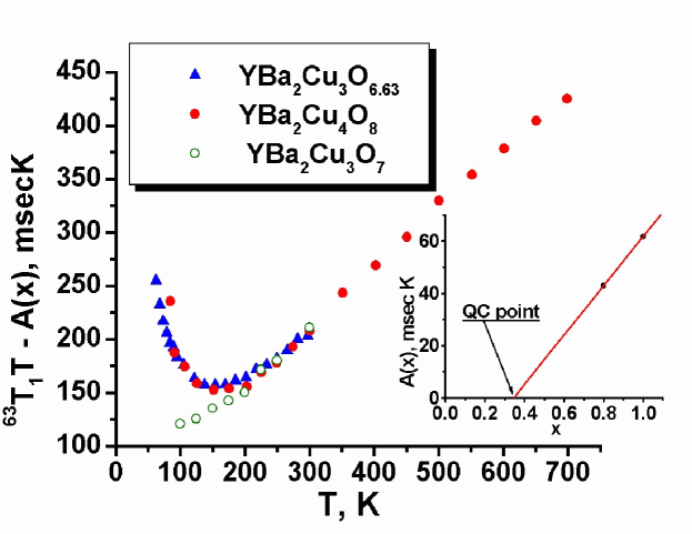
Figure 34: Scaling for the NMR relaxation rate $T_{1}$ in YBa₂Cu₃O_6+x. The offset $A(x)$ shown in the inset depends linearly on $x$, and points to a QCP in the spin liquid.

The long range magnetic order at $x<0.05$ can be a 2D antiferromagnet or a spin glass[3].

While the details of the microscopic theory at low doping may vary, the experimental data imply the presence of a linear spin wave-type excitation spectrum in the spin liquid with a temperature-dependent gap, $\Delta_{SL}(x,T)$, that is controlled by its distance from the quantum critical point at $x=0.05$. The spin wave excitation spectrum has the following form:

$$\epsilon(\bm{q})=\sqrt{\Delta_{SL}^{2}+c^{2}(\bm{q}-\bm{Q})^{2}},\ \ \Delta_{SL}=\frac{c}{\xi(T,x)}\,.$$ (84)

Here $c$ is the spin wave velocity. In the $z=1$ QC regime the spin gap $\Delta_{SL}$ tracks $\omega_{SF}=c^{\prime}/\xi$. For $x>0.05$ the gap saturates at low temperatures to $\Delta_{0}=c/\xi_{0}(x)$ at the crossover to the QD gapped spin liquid regime. We note that the origin of the saturation of the correlation length is largely irrelevant for data analysis - an energy gap can appear in the 2D quantum spin liquid[47, 48], or in 1D stripes of spin liquid[61] due to dimensional crossover. In the latter case the correlation length will saturate at the size of the domain or dynamic stripe order, $\xi(T=0)\propto L$. Therefore, experiment does not distinguish between these possibilities.

The QC-QD crossover could explain the sharp upturn in ${}^{63}T_{1}T$ at low temperatures observed in NMR experiments on 1-2-3 materials at temperatures well above $T_{c}$ that is not found in experiments on the 2-1-4 materials. Since $c(x)\propto T^{m}(x)$, and becomes small as one approaches $x=0.22$, while $1/\xi_{0}(x)$ increases linearly from $x=0.05$, the zero-temperature spin liquid gap $\Delta_{0}\equiv\Delta_{SL}(x,0)$ will have a bell-shaped form similar to $T_{c}(x)$. The gapping of the spin liquid leads to an exponential decrease of damping with temperature in the spin liquid.

The detailed properties of the spin liquid can be extracted directly from the NMR ${}^{63}T_{1}$ relaxation rates measurements using the ansatz for the correlation length $\xi(T^{m})=1$, or, where these exist, from both ${}^{63}T_{1}$ and ${}^{63}T_{2G}$ measurements, as it was shown some time ago by the authors[9]. In the $z=1$ QC regime,

$${}^{63}T_{1}T \propto \frac{\omega_{SF}}{\alpha(x)f(x)}\,,$$ (85)

$$\frac{1}{{}^{63}T_{2G}}\, \propto \alpha(x)f(x)\xi,$$ (86)

where all parameters are taken from Eq.(53); these equations differ from those in Ref. [9] by the presence of an extra factor $f(x)$ in Eq.(53). A combination of these two measurements[9] gives a handle on the spin wave velocity $c$:

$$\frac{{}^{63}T_{1}T}{{}^{63}T_{2G}}\,\propto\omega_{SF}\xi\equiv c^{\prime}\simeq 0.55c$$ (87)

The coefficients of proportionality are given by the hyperfine Hamiltonian. As easily seen from the above equations,

$${}^{63}T_{1}(T^{m})T^{m}\propto\frac{c^{\prime}}{f(x)\alpha(x)}\,.$$ (88)

The high-temperature scaling for ${}^{63}T_{1}$, ${}^{63}T_{1}(T)=const$, that was seen by Imai et al.[18] in La_2-xSr_xCuO₄, but is not present in the 1-2-3 materials, at first sight seems to imply $x$-independent exchange integral, $J$, or $c^{\prime}$, which contradicts the bulk susceptibility data for this material. However, a closer look shows there is no contradiction. As we have seen in Section 3.1, $f(x)$ and $T^{m}(x)$ both depend linearly on $x$. Thus, on general grounds, one can write:

$$c^{\prime}(x)\propto c(x)\propto T^{m}(x)\propto\alpha^{-1}(x)\propto f(x).$$ (89)

The Imai et al.[18] scaling then follows from Eq.(88), since one can approximately write:

$$\alpha(x)f(x)\simeq\alpha(0)\simeq 11.3states/eV$$ (90)

In general, the empirical scaling of Eq.(89) is somewhat accidental, since the low-energy properties of the spin liquid can be renormalized by interaction with fermionic quasiparticle excitations. This renormalization appears to be small for the 2-1-4 materials but appears to be important for the 1-2-3 materials, where the Ohsugi et al.[49] results and the Imai et al.[18] high-temperature scaling of ${}^{63}T_{1}$ are not observed. $f(x)$, $T^{m}(x)$, and $c^{\prime}(x)$ can in principle be independently determined from NMR experiments. Since ${}^{63}T_{2G}$ has only been measured for the YBa₂Cu₃O_6+x family, we plot the doping dependence of $c^{\prime}$ for these materials in Fig. 35, assuming commensurate local spin response.

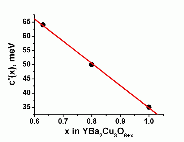
Figure 35: $c^{\prime}(x)$ from NMR experiments in YBa₂Cu₃O_6+x

It is evident that $c^{\prime}(x)$ decreases approximately linearly with doping. However, a comparison of $c^{\prime}(x)$ with $T^{m}(x)$ shows that the two quantities do not track each other, violating the empirical scaling of Eq.(89). While the doping dependence for both is linear, it is evident from Fig.36 that they are not proportional to one another. The violation of the Imai et al.[18] scaling relation by this family of materials is therefore to be expected.

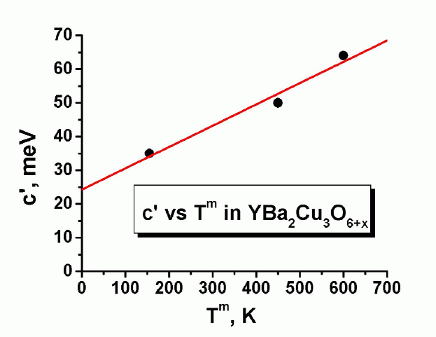
Figure 36: $c^{\prime}(x)$ vs $T^{m}(x)$ from NMR experiments in YBa₂Cu₃O_6+x

The doping dependence of the parameter $c^{\prime}(x)/f(x)\alpha(x)$, that follows from NMR ${}^{63}T_{1}$ measurements only, is shown in Figs 37,38. We see that the empirical scaling relation Eq.(90) holds reasonably well for the La_2-xSr_xCuO₄ family, so that the doping dependence of this parameter also yields the doping dependence of $c(x)$.

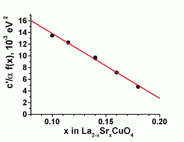
Figure 37: $c^{\prime}(x)/f(x)\alpha(x)$ from NMR experiments in La_2-xSr_xCuO₄

Figure 38: $c^{\prime}(x)/f(x)\alpha(x)$ vs $T^{m}(x)$ from NMR experiments in La_2-xSr_xCuO₄

3.5 Thermodynamics

We now turn to an analysis of thermodynamic measurements of the electronic entropy[16]. These are quite difficult to carry out, since the phonon contribution accounts for 98-99 % of the measured value of the entropy, and must be subtracted to a high degree of accuracy to get the electronic contribution. The subtraction procedure is a complicated process, involving subtracting data for a reference material, such as YBa₂Cu₃O₆[16], and making additional corrections for the modification of the phonon DOS with doping. The reference material is usually an insulator, either the parent compound, or a compound in which the Fermi liquid is suppressed with impurities such as Zn. The difficulty with such a subtraction procedure for analyzing the data is that the spin liquid contribution exists even when the Fermi liquid is suppressed. Thus, a consistent data analysis requires that the reference material be known. For this reason we restrict our attention to the data of Ref.[16], where the reference material is YBa₂Cu₃O₆. The spin liquid contribution of the parent compound is subtracted from the electronic entropy in this analysis. Nevertheless, at moderate temperatures $T<300K$ it remains comparatively small.

Our analysis of the data of Ref.[16] shows that the entropy displays scaling and two component behavior in the form:

$$S=f(x)S_{SL}(T/T^{m})+(1-f(x))\gamma T,$$ (91)

with a scaling function $S_{SL}(T/T^{m})$ that corresponds to the theoretically calculated entropy for the Heisenberg model[5].

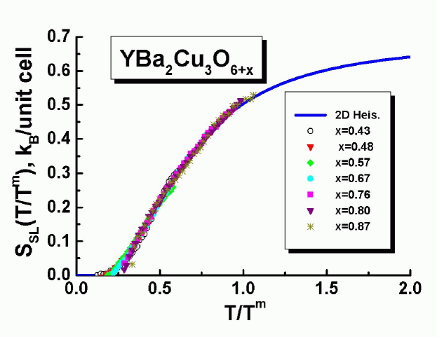
Figure 39: Scaling for the spin liquid part of the entropy $S_{SL}(T/T^{m})$ in YBa₂Cu₃O_6+x. The entropy data is from Ref.[16] in the intermediate doping regime, where the spin liquid part of the entropy is not subtracted. $T^{m}(x)$ and $f(x)$ obtained from this analysis are consistent with our analysis of the NMR Knight shift and the bulk spin susceptibility. The solid line is the integrated numerical result for the heat capacity of the 2D Heisenberg model taken from Ref. [5].

We have integrated the numerical results for the heat capacity of the Heisenberg model from Ref.[5] to get the expected entropy. We show the results of this analysis and the data collapse on the Heisenberg scaling curve in Fig.39. We find that at small doping scaling becomes progressively worse, as might be expected because of the subtraction procedure followed.

To understand our result, we note that on general grounds, one can write the entropy in the form:

$$S=f(x)S_{SL}+(1-f(x))S_{FL}+S_{config},$$ (92)

where $S_{config}$ is the configurational entropy of the fluctuating stripe or domain order discussed in the next subsection. The configurational part, however, is not seen in the data factorization Eq.(91) We believe, the reason for this is that the configurational contribution of the fluctuating stripes could also be linear in temperature[111]. Indeed, the domain walls can be treated as solitons, with the Hamiltonian

$$H_{s}=\frac{1}{2}\,\epsilon_{0}\int dy\left(\frac{du}{dy}\,\right)^{2},$$ (93)

where $y$ is the direction along the stripe, while $u$ is the displacement of the wall perpendicular to its equilibrium direction; $\epsilon_{0}$ is the linear tension of the domain wall (soliton). This model maps on a 1D fermion model[111, 112], and the resulting configurational entropy has a linear form,

$$S_{config}=\frac{\pi^{2}}{3}\,\frac{T}{\epsilon_{0}l^{2}}\,,$$ (94)

where $l$ is the mean distance between solitons. Such a linear contribution to the entropy is indistinguishable from the Fermi liquid contribution.

3.6 Inelastic neutron scattering

Our analysis also casts light on the issue of intrinsic spatial inhomogeneity[53] in the pseudogap state[79, 61]. The issue is how to reconcile the commensurate spin susceptibility peaks required by the spin liquid and the fit to the NMR data[36], with the incommensurate peaks seen in inelastic neutron scattering experiments[26]. The oxygen relaxation rate is known to be very small compared to copper, with a very different modified Korringa-type temperature dependence. An attempt to explain it within the one-component model with incommensurate spin liquid peaks[36, 45] in La_1.85Sr_0.15CuO₄ leads to an oxygen relaxation rate that is a factor of three too large compared with actual experimental data, and has the wrong temperature dependence.

Similar inconsistencies occur with relaxation rates on other nuclei, such as $O$ or $Y$ in YBa₂Cu₃O_6+x. The contradiction cannot be resolved if one assumes two different components sitting on oxygen and copper. Indeed, since the Knight shift on different nuclei has an identical temperature dependence[34, 39], it requires the existence of a transferred hyperfine coupling from the copper[32]. Such a transferred hyperfine interaction assumed by MMP will, however, induce a ”leakage” spin liquid contribution from the spin liquid in the two-component picture for any incommensurate spin liquid response.

The resolution was suggested some time ago by Slichter[44], who pointed out that if, as a result of Coulomb interaction between the holes, regions that were hole rich formed domain walls between regions in which one had nearly antiferromagnetic commensurate behavior, the two kinds of experiments were compatible. This issue has been independently confirmed and clarified by Tranquadaet al.[79, 61], who found that the spin wave dispersion seen in cuprate superconductors by inelastic neutron scattering is consistent with commensurate spin response of a spin ladder, while the incommensurate structure appears as a result of the fluctuating stripe order.

Such a scenario implies finite-size scaling, and saturation of the antiferromagnetic correlation length at low temperatures at a value of the order of the size of the domain. Estimating the size of the domain from the discommensuration seen in neutron scattering experiments[26] in La_1.86Sr_0.14CuO₄, $\delta q=\pi\delta$, $\delta=0.245$, we can write:

$$\delta qL=2\pi=\pi\delta L$$ (95)

Thus,

$$L/a=\frac{2}{\delta}\,=8.16,$$ (96)

where $a$ is the lattice spacing. Aeppli et al.[26] find the saturated correlation length in La_2-xSr_xCuO₄ at a doping level of $x=0.14$ is

$$\xi_{0}=29.4\AA=7.7a,$$ (97)

a value that is very close to our estimate of $L$. We conclude that both magnetic probes imply the presence of a fluctuating striped or other domain order. Apart from the issue of incommensurate peaks seen in INS experiments and its possible resolution in terms of a fluctuating domain order, the spin wave spectrum and the correlation length observed in inelastic neutron scattering experiments is completely consistent with our proposed two-fluid scenario, as we show below.

We return now to the magnetic scaling seen in the inelastic neutron scattering experiments which, like the ${}^{63}Cu$ NMR relaxation rates, probe spin liquid behavior. We begin with the experiments of Sternlieb et al.[25] that imply the presence of a true $\omega/T$ scaling for the local spin susceptibility in the underdoped material YBa₂Cu₃O_6.6. The data collapse observed experimentally can be fit to the following simple scaling form:

$$\chi_{L}^{\prime\prime}(\omega,T)=A(x)\frac{\omega}{T}\,,$$ (98)

with deviations from scaling that occur at progressively lower temperatures, as the frequency $\omega$ increases.

This scaling confirms the high-temperature scaling seen in NMR[18]. To clarify this point, we plot both experimental results in the same units in Fig. 40. The quantity measured in neutron scattering experiments analogous to ${}^{63}T_{1}T\propto\omega_{SF}$ is a function of the local spin response, $\omega/\chi^{\prime\prime}_{L}(\omega,T)$, typically given in counts/minute. We therefore fix the absolute value of that response to be consistent with high-temperature NMR.

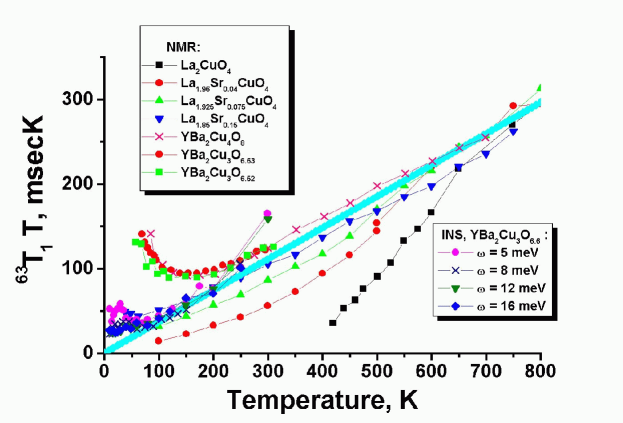
Figure 40: Local spin response seen in inelastic neutron scattering in YBa₂Cu₃O_6.6, $\omega/\chi^{\prime\prime}_{L}(\omega,T)$ , scaled to NMR ${}^{63}T_{1}T$ in La_2-xSr_xCuO₄ and YBa₂Cu₃O_6+x.

Both experiments reveal linear in temperature $\omega_{SF}$, a signature of magnetic quantum critical behavior. At finite frequencies this regime extends to lower temperatures, as one may expect on general grounds.

The presence of $z=1$ quantum critical behavior is verified further by the INS measurements of the temperature dependence of the correlation length seen in La_1.86Sr_0.14CuO₄[26]. Aeppli et al.[26] show that

$$\frac{1}{\xi^{2}}\,=\frac{1}{\xi_{0}^{2}}\,+\frac{a_{0}^{-2}}{\Gamma^{2}}\,[(k_{B}T)^{2}+(\hbar\omega)^{2}],$$ (99)

where $\xi_{0}=29.4\AA$, $\Gamma\simeq 47meV$. For the QC scaling in the $\sigma$-model[47, 48],

$$\frac{c}{\xi}\,=1.04k_{B}T.$$ (100)

On the other hand, the Aeppli et al.[26] result gives, if $\xi$ is measured in lattice constants:

$$\frac{1}{\xi}\,\simeq\frac{k_{B}T}{\Gamma}\,,$$ (101)

Thus, for $x=0.14$ we find

$$c=1.04\Gamma=49meV,$$ (102)

a value that is much less than that found for the insulator value $c_{ins}=224meV$, and is qualitatively consistent with the behavior of the effective $J$ inferred from the bulk spin susceptibility measurements.

Another comparison of theory with experiment on the spin liquid phase diagram comes from the neutron scattering measurements of the magnetic correlation length. For the Heisenberg spin liquid, the correlation length $\xi=1$ at $T\simeq T^{m}$. On using the results for $\xi$ obtained by Aeppli et al., we find:

$$T(\xi=1)=T^{m}(x=0.14)=540K\pm 100K.$$ (103)

In good agreement with the result, $T^{m}=460K$, at $x=0.14$ doping obtained using Eq.(76).

A further important point that follows from the results of Aeppli et al.[26] concerns the breakdown of scaling, which should occur at a universal scale $T_{a}$, such that

$$k_{B}T_{a}=\sqrt{(\hbar\omega)^{2}+(k_{B}T_{br}(\omega))^{2}},$$ (104)

where $T_{br}$ is the temperature of the breakdown of $\omega/T$ scaling seen in the neutron scattering experiments at a fixed frequency $\omega$. NMR experiments just measure $T_{a}$ directly. We analyze the data of Sternlieb et al.[25] using this framework to see if it is consistent with the results shown in Fig. 41.

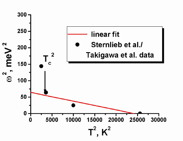
Figure 41: Temperature-frequency analysis of scaling failure, data from Sternlieb et al. and Takigawa (6.63 NMR)

According to Aeppli et al., the breakdown of scaling frequency/temperature can be fit to the form:

$$\omega^{2}_{br}=E_{br}^{2}-AT_{br}^{2}$$ (105)

From this analysis we find, for YBaCuO_6.6:

$$E_{br}=8.03meV,\ \ A=-0.00256(meV^{2}/K^{2}),$$ (106)

or

$$\omega_{br}(T=0) = 8.03meV=93K,$$ (107)

$$T_{br}(\omega=0)=T^{m}/3 = 159K,$$ (108)

$$\frac{\omega_{br}}{T_{br}}\, = 0.58.$$ (109)

Overall, this experimental picture is self-consistent, although the experimental finding of the simple form for the breakdown Eq. (105) is rather surprising.

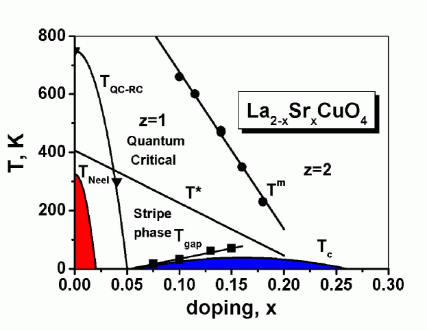
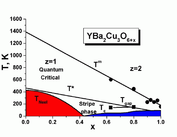
Figure 42: (a) The spin liquid phase diagram for La_2-xSr_xCuO₄. $T^{m}(x)$ corresponds to a crossover at $\xi(T,x)=1$ to the strongly correlated phase in the spin liquid. $T^{*}(x)\simeq T^{m}(x)/3$ corresponds to the appearance of fluctuating stripe order $T_{gap}$ marks the spin liquid crossover from the quantum critical (QC) to quantum disordered (QD), or gapped spin liquid, regime in the stripe phase. $T_{QC-RC}$ is the spin liquid crossover from the QC to renormalized classical (RC) regime. (b) The spin liquid phase diagram for YBa₂Cu₃O_6+x displays similar crossovers.

We conclude this section with a brief discussion of phase diagram for the spin liquid that is consistent with the experimental constraints discussed above. Our proposed phase diagram[3] is shown in Fig.42.

The phase transition or a crossover at a doping level $\sim 0.22$ is that from the conducting Fermi liquid on the right-hand side to pseudogap matter on the left-hand side, in which a portion of the quasiparticle Fermi surface has lost its low-frequency spectral weight, becoming localized in an insulating spin liquid that coexists with the remaining Fermi liquid component. The two interacting components are present at all temperatures in the underdoped regime, $x<0.22$. At high temperatures $T>T^{*}\simeq T^{m}/3$ the interaction leads to a modification of $J$, the effective exchange interaction in the spin liquid, while the Fermi liquid component remains intact. As the temperature is lowered, the growth of correlation length in the spin liquid results in stronger renormalization of the Fermi liquid component, and the formation of the Fermi arcs at temperatures $T<T^{*}\simeq T^{m}/3$. The antiferromagnetic correlation length also becomes finite at low temperatures, which results in a gap for the spin excitation spectrum at $\bm{Q}=(\pi,\pi)$. The quantum critical point at $x\sim 0.05$ corresponds to a quantum transition between two different states of the spin liquid.

We now return to the question of how close the measured spin liquid maps onto the Heisenberg spin liquid. While there is a one to one correspondence for the static spin susceptibility above $T\simeq T^{*}$, the difference becomes large at lower temperatures, where the correlation length $\xi$ and the spin liquid gap $\Delta_{SL}$ saturate at a finite value. Presumably it is this difference that is responsible for the mild departure in concentration dependences deduced for $f(x)$ and $T^{m}(x)$.

4 Discussion

Given the presence of both a spin liquid and a Fermi liquid in the normal state of underdoped superconductors, it is natural to consider their interaction as being responsible for their anomalous normal state properties and the transition to a gapped quantum state at $T^{*}$ and to superconductivity at $T_{c}$. We begin by considering the extent to which the observed scaling behavior reflects that interaction, and what might be some of its other consequences.

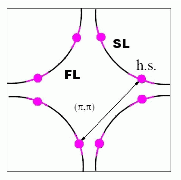
Figure 43: Hot regions near spots on the Fermi surface separated by wavevector $\bm{Q}=(\pi,\pi)$ and cold regions away from the hot spots

From an examination of the experimental results presented in the previous sections we draw the following conclusions:

(i) The scaling with $T^{m}$ of various transport properties of the non-Landau Fermi liquid tells us that the transport properties in the normal state of the cuprate superconductors are dominated by the magnetic coupling between the quasiparticles and the spin liquid excitations

(ii) In the 1-2-3 materials, the scaling of $T^{*}$ and $\Delta_{g}$, the d-wave energy gap found below $T^{*}$ for quasiparticles located in the ”hot” regions of the Fermi surface, and below $T_{c}$ for the remaining ”cold” or nodal quasiparticles, tells us that the physical mechanism for their gaps and subsequent superconductivity must be magnetic.

(iii) As may be seen in Fig.43, the hot regions seen in the ARPES experiments are defined by their proximity to points on the Fermi surface that are separated by commensurate wavevectors, $\bm{Q}=(\pi,\pi)$; their physical location tells us that the magnetic interactions responsible for the gap must be peaked at $\bm{Q}$. This is to be expected if the ”glue” for the quasiparticle interaction is provided by the spin liquid excitations of the Heisenberg model that exhibit the MMP form with a strong peak at $\bm{Q}$, since their coupling to the Fermi liquid yields an induced quasiparticle interaction that is likewise peaked at $\bm{Q}$. Moreover, in agreement with the early models of spin-fluctuation-induced superconductivity[113, 114, 115] the resulting energy gaps will be d-wave.

(iv) The penetration-depth measurements of the doping-dependence of the of the superconducting condensate tell us that where present in the underdoped materials, the spin liquid does not participate in their superconductivity.

(v) The fact that the scaling relations below $T^{m}$ for a pure Heisenberg model are much better obeyed in the 2-1-4 materials than in the 1-2-3 materials tells us that the influence of the hot quasiparticles on the spin liquid is considerably weaker in the 2-1-4 materials.

(vi) Since the spin liquid excitations in the two classes of materials are quite similar, these differences plausibly arise from band-structure effects[116, 117] that reduce the importance of hot spots on their Fermi surface.

(vii) These last conclusions concerning the relative strengths of the coupling of hot quasiparticles to the spin liquid and their spin-fluctuation-induced quasiparticle interaction in the 1-2-3 and 2-1-4 materials provide a simple physical explanation of some of the major differences between their physical behavior of the two classes of materials. It is why the 2-1-4 materials show no indications of either a spin fluctuation gap or a quasiparticle gap opening up at $T^{*}$, and may be related to their significantly lower superconducting transition temperatures.

(viii) There are many indications that ”stripy” behavior is more prevalent in the 2-1-4 materials; this may be due to the fact that the fluctuating domains become well established only when fairly strong AF correlations are present. For the 1-2-3 materials gaps open up at $T\sim T^{m}/3$, so the maximum AF correlation length one expects to find is $\sim 3$ lattice spacings; for the 2-1-4 materials, on the other hand, one finds AF correlation lengths $\sim 8$ lattice spacings near optimal doping and still longer correlation lengths are to be expected for the underdoped materials.

(ix) Experiment indicates that at low temperatures $T\sim T^{*}\simeq T^{m}/3$, charge fluctuations, domains, and tendencies toward phase separation all play an important role, although the two-component nature is present in the underdoped regime at all temperatures, and is therefore intrinsic.

(x) Our two-fluid model provides a natural way to develop a phenomenological description of stripe formation at low frequencies, since all that is required is to let $f(x)$ vary periodically in space and time.

We conclude this section with a brief discussion of some necessary elements of a microscopic description of the spin and Fermi liquids. We note first that for the spin liquid, the AF critical point at $x\simeq 0.05$ is responsible for the observed $z=1$ QC behavior. The spin liquid component at temperatures $T>T^{*}$ is well described to first approximation by the standard bosonic $\phi^{4}$ Hertz-Millis theory of quantum critical behavior[118, 119]. For $\xi>1$ one is outside the critical region, in the vicinity of weak-coupling Gaussian fixed point, where fluctuation corrections are not important. The standard damping due to its interaction with fermions gives rise to the $z=2$ mean field Ornstein-Zernike/MMP form. In the critical region $\phi^{4}$ theory becomes equivalent to the QNL$\sigma$ model[47, 48] (the two theories differ by an irrelevant operator). However, at low correlation lengths the irrelevant operator of the $\phi^{4}$ theory plays a crucial role, inducing a crossover to the mean field Gaussian regime[9] with $\xi\propto T^{-1/2}$ for $N=\infty$ version[120]. Such $z=1$ to $z=2$ mean field crossover cannot be obtained in the quantum non-linear $\sigma$-model with fermionic damping[121].

There appear to be two kinds of departures from the simple Heisenberg description. The first concerns the static bulk susceptibility that falls below the currently calculated values for the Heisenberg model for $T<T^{m}/3$. Because this fall-off is essentially the same in both the 2-1-4 and 1-2-3 materials, it is likely not brought about by spin-fermion coupling, since that coupling is quite different for the two materials. It could represent an inadequacy in the calculations of the expected behavior of the Heisenberg model at these low temperatures. The second concerns the opening up of a gap in the low frequency spin liquid excitation spectrum at $(\pi,\pi)$ that is seen as a minimum in $T_{1}T$ at $150K\simeq 0.31T^{m}$ in the NMR experiments on the 1-2-4 material and at $140K\simeq 0.23T^{m}$ in the YBa₂Cu₃O_6.63 material. It is plausible to conclude that it reflects a reduction in quasiparticle damping brought about by the onset of the hot quasi-particle gapped behavior at $T^{*}$. However,it would then seem that the transition to this new quantum state is not universal, i.e. does not always occur at a fixed fraction of $T^{m}$. Indeed these NMR-determined onset temperatures, $T^{*}$, scale, to first approximation with $T_{c}$; thus for the 1-2-4 material one has $T^{*}\simeq 2.1T_{c}$, while for YBa₂Cu₃0_6.63 one finds $T^{*}\simeq 2.3T_{c}$. Based on these estimates, and those obtained from the ARPES and STM experiments on 2212 members of the 1-2-3 family , our candidate phase diagram for the 1-2-3 materials is given in Fig. 42b. It differs from the corresponding diagram for the 214 materials in the presence of a ”high temperature” transition at $T^{*}$ to the gapped quantum state.

In considering microscopic models for the evolution of Fermi liquid behavior with doping, we begin by recalling that high-T_c superconductors are doped charge-transfer insulators[122, 123]. Thus, an adequate starting point for a description of the CuO₂ planes follows from their chemistry, and is the three-band Hubbard model composed of 3 d${}_{x^{2}-y^{2}}$ orbitals on the Cu site and 2 p_x,y orbitals on the O sites[124, 125, 126]. The two key parameters of the three-band Hubbard model are are the charge-transfer energy $E_{CT}=\epsilon_{p}-\epsilon_{d}$, and the copper on-site Coulomb repulsion, $U_{d}$. In the limit of strong p-d hybridization and very strong on-site Cu Coulomb interaction, the model gives rise to 5 different bands: an antibonding band, further split into upper Hubbard band (Cu $d^{10}$ configuration), and lower Hubbard band (Cu $d^{8}$ configuration) by the Coulomb interaction, a bonding band, further split into Zhang-Rice (ZR)[35] singlet and triplet bands, and the non-bonding oxygen band.

Following Anderson[97], most theoretical studies have considered a simpler one band Hubbard model, which has fewer parameters and assumes that the low-energy physics of the electronic states in the vicinity of the charge-transfer gap is described well by taking a relevant low-energy subset of this complex band structure, the ZR singlet band and the upper Hubbard band, separated by $U\simeq E_{CT}\sim 1.7eV$ of the order of the charge-transfer gap. Numerical studies of the three-band Hubbard model[127] support such reduction. The two low-energy bands of the effective single-band Hubbard model are strongly correlated hybridized copper-oxygen bands, with the upper Hubbard band having mostly oxygen character[128, 129, 116, 117].

However, on the basis of numerical LDA calculations, it has been suggested that a single-band tight binding model may not provide a sufficiently good qualitative description of the many bands involved[116, 117]. Moreover, we have seen that $\chi_{dd}$ contains the spin liquid component localized on the copper sites, while $\chi_{pd}$ and $\chi_{pp}$ pick up contributions from the holes on the oxygen sites. The difference in relevant form factors could potentially explain many anomalies observed for NMR relaxation rates[36] and inelastic neutron scattering experiments, as we have discussed in the previous section.

The analogy with two-fluid model for heavy fermions[101, 102] can be better understood from an alternative approach to three-band Hubbard model[124, 125, 126], that is perturbative in p-d hybridization, $t_{pd}$. In case of exactly one hole per Cu and strong Hubbard Coulomb on-site repulsion $U_{d}$, the low-energy Hamiltonian for the three-band Hubbard model reduces to the Heisenberg spin Hamiltonian with exchange coupling

$$J_{H}=\frac{4t_{pd}^{4}}{(E_{CT}+U_{pd})^{2}}\,\left(\frac{1}{U_{d}}\,+\frac{2}{2E_{CT}+U_{p}}\,\right),$$ (110)

since the charge excitations have a gap $E_{CT}^{g}\simeq 1.7eV$. Numerical calculations for the three-band Hubbard model[127] extract the value $J_{H}\simeq 0.13eV$, consistent with that observed in neutron scattering experiments. The oxygen holes and the nearest $Cu$ spin interact via a strong Kondo exchange interaction, which can be obtained in perturbation theory in $t_{pd}/E_{CT}$,

$$J_{K}=t_{pd}^{2}\left(\frac{1}{E_{CT}}\,+\frac{1}{U_{d}-E_{CT}}\right).$$ (111)

The perturbative analysis of the three-band Hubbard model reduces it to the spin-fermion model via the Schrieffer-Wolff[130] transformation,

$$H_{SF}=\sum_{j,j^{\prime},\sigma}t_{jj^{\prime}}c^{\dagger}_{j\sigma}c_{j^{\prime}\sigma}+\sum_{j,j^{\prime},i,\sigma,\sigma^{\prime}}J_{K}(j,j^{\prime},i)c^{\dagger}_{j\sigma}\bm{\sigma}_{\sigma\sigma^{\prime}}\bm{S}_{i}c_{j^{\prime},\sigma^{\prime}}+J_{H}\sum_{i,i^{\prime}}\bm{S}_{i}\bm{S}_{i^{\prime}}.$$ (112)

Here the index $i$($j$) runs over Cu (O) sites, $c^{\dagger}_{j\sigma}$, $c_{j\sigma}$ are creation and annihilation operators, respectively, for holes in oxygen p bands. The Kondo interaction is, in general, non-local[125]. The Hamiltonian Eq.(112) is the Kondo-Heisenberg model, known for the periodic Anderson model in many physical systems, including magnetic semiconductors[131], heavy fermions (the Kondo lattice model)[130], and high-T_c superconductors[124, 125]. The heavy fermion materials and high-$T_{c}$ materials correspond to different limits of the model Eq.(112). In heavy fermion superconductors the Kondo interaction $J_{K}$ is initially comparatively small, and gets renormalized by the conduction band as the temperature is lowered, leading to the onset of coherence at $T^{*}$, and the two-fluid heavy fermion behavior[101, 102, 132] with a temperature-dependent fraction of spin liquid (spin impurity contribution). The high-$T_{c}$ superconductors, on the other hand, are in the strong-coupling Zhang-Rice[35] limit of the same microscopic model, Eq.(112). The Kondo interaction is very large, $J_{K}\sim 0.7eV$, which leads to a formation and propagation of the “Zhang-Rice singlets”, reducing the microscopic Hamiltonian to an effective one-band $t-J$ model[97]. The projection operators of the Zhang-Rice singlet[35] automatically imply that $\chi_{pd}=\chi_{pp}=0$. Thus, as suggested by MMP[40], different nuclei then feel the presence of a single temperature-dependent spin component residing on copper, or $\chi_{dd}$. The Zhang-Rice singlet picture (and the t-J model), however, inevitably gets violated at higher doping, as a single large Fermi surface develops, that corresponds to antibonding p-d hybridized band. A linear decrease of effective $J(x)$ with increased doping $x$ is “high-energy physics”, as is evident from, for example, an adiabatic treatment of the t-J model[133]. Thus, the fraction of spin liquid[3] observed in “low energy” experiments on the cuprate superconductors will be temperature-independent. In heavy fermion metals it is the mixed $c-f$ contribution, $\chi_{cf}(T)=(1-f(T))\chi_{FL}(T)$, that gives rise to the heavy Fermi liquid contribution[102]. In high-temperature superconductors, on the other hand, one normally uses the Zhang-Rice singlet band and the upper Hubbard band of the three-band Hubbard model as lower and upper Hubbard bands of the effective single-band Hubbard Hamiltonian. Using the analogy the heavy fermion two-fluid model[101, 102] and the two-fluid model for high-T_c superconductors, the Fermi liquid contribution in the cuprates should arise from $\chi_{pd}$ and $\chi_{pp}$ parts of the bulk spin susceptibility, which, strictly speaking, indicates a violation of the Zhang-Rice singlet picture at high doping, given by Eqs. (50), (51). Since the effective mass of carriers is not heavy in high-$T_{c}$ superconductors, one would expect both $\chi_{pp}$ and $\chi_{pd}$ contributions to be present. This result contrasts strongly with the pure Zhang-Rice[35] limit in which all contributions arise from $\chi_{dd}$[40]. The key answer to this very important question is held by the new Knight shift experiments[102, 39], since then Knight shifts on different nuclei should see a different temperature dependence, at least below the superconducting temperature, $T_{c}$.

5 Conclusion

Our review of scaling behavior in the cuprate superconductors makes evident the critical role that the localization of Cu spins by strong on-site repulsive Coulomb interactions plays in determining the properties of the magnetically underdoped superconductors, those whose planar hole concentrations are $<0.20$. While there is much more in the way of details that experiment can and will provide, from additional c-axis NMR experiments on 1-2-3 materials that enable one to follow the emergence of a distinct Fermi liquid contribution, to ARPES, NMR , and STM experiments that fill in the details of the emergence of the gapped hot quasiparticle state at $T^{*}$, we believe that the overall low-energy physical picture of a normal state described by two fluids whose interaction leads to its remarkable properties has now been firmly established.

It is equally clear that much much more remains to be done, beginning with the development of a better microscopic foundation for the physical picture that experiment has ”forced” upon us, and an improved treatment of transport processes based upon it. We mention here but a few of the many remaining challenges and mysteries that surround these fascinating materials:

(i) There are striking similarities in the doping dependence of $T_{c}$ in the 1-2-3 and 2-1-4 materials despite the difference in their spin-fermion couplings and the magnitudes of their respective transition temperatures. Does this tell us that these differences are primarily in how the hot quasiparticles couple to spin fluctuations and that the spin-fermion couplings for the cold quasiparticles that bring on their superconductivity can somehow be scaled for these two classes of materials?

(ii) Although the spin liquid ceases to be a significant ”player” for doping levels greater than, say, $0.20$, the existence of a smooth cross-over in most physical properties of the normal state, including the superconducting transition, as one goes from magnetically underdoped to magnetically overdoped materials, suggests that its disappearance must be accompanied by the emergence of sufficiently strong antiferromagnetic correlations in the Fermi liquid that enable its properties to merge smoothly with those induced by the spin liquid. Can these be detected experimentally and understood microscopically? Might the disappearance of the spin liquid be accompanied by the emergence of a single-band Hubbard model that is valid for the overdoped materials?

(iii) Do the gapped hot quasiparticles found below $T^{*}$ in the 1-2-3 materials become effectively localized and so become part of the spin liquid? Is there any way to make their gapping more productive, in terms of their becoming part of the superconducting condensate, thereby opening the way to a superconducting transition at the considerably higher transition temperature, $T^{*}$?

(iv) Can the lessons learned from the cuprates be transferred to other materials, and so lead over time to the discovery of still higher temperature superconductors?

6 Acknowledgements

We would like to thank E. Abrahams, N. Curro, L.P. Gor’kov, J. Haase, J. Schmalian, and C.P. Slichter for stimulating discussions, and acknowledge support for VB from NHMFL through the NSF Cooperative agreement No. DMR-008473 and for DP from the Institute for Complex Adaptive Matter and the US Department of Energy.

References

- [1] M. R. Norman, D. Pines, and C. Kallin, Adv. Phys. 54, 715 (2005).
- [2] D. C. Johnston, Phys. Rev. Lett. 62, 957 (1989).
- [3] V. Barzykin, D. Pines, Phys. Rev. Lett.96, 247002 (2006).
- [4] S. Hüfner, M.A. Hossain, A. Damascelli, and G.A. Sawatzky, Rep. Prog. Phys. 71, 062501 (2008).
- [5] M.S. Makivić and H-Q Ding, Phys. Rev. B 43, 3562 (1990).
- [6] A. Kanigel, M.R. Norman, M. Randeria, U. Chatterjee, S. Souma, A. Kaminski, H.M. Fretwell, S. Rosenkranz, M. Shi, T. Sato, T. Takahashi, Z.Z. Li, H. Raffy, K. Kadowaki, D. Hinks, L. Ozyuzer, and J.C. Campuzano, Nature Physics 2, 447 (2006).
- [7] J. W. Alldredge, J. Lee, K. McElroy, M. Wang, K. Fujita, Y. Kohsaka, C. Taylor, H. Eisaki, S. Uchida, P.J. Hirschfeld, and J.C. David, Nature Physics 4, 319 (2008).
- [8] K.K.Gomes, A.N. Pasupathy, A. Pushp, S. Ono, Y. Ando, A Yazdani, Nature 447, 569 (2007).
- [9] V. Barzykin and D. Pines, Phys. Rev. B 52, 13585 (1995).
- [10] J. G. Bednorz and K. A. Müller, Z. Phys. B 64, 189 (1986).
- [11] T. Nakano, M. Oda, C. Manabe, N. Momono, Y. Miura, and M. Ido, Phys.Rev. B 49, 16000 (1994).
- [12] M. Oda, H. Matsuki, and M. Ido, Solid State Commun 74, 1321 (1990).
- [13] B. Wuyts, V. V. Moshchalkov, and Y. Bruynseraede, Phys. Rev. B 53, 9418 (1996).
- [14] H. Alloul, Physica B 169, 51 (1991).
- [15] N. Curro, Z. Fisk, D. Pines, MRS bulletin 30, 442 (2005).
- [16] J. Loram, K.A. Mirza, J.R. Cooper, and W.Y. Liang, Phys. Rev. Lett. 71, 1740 (1993); J. W. Loram, K. A. Mirza, J. R. Cooper, W. Y. Liang, and J. M. Wade, J. Supercond. 7, 243 (1994).
- [17] J. L. Talon, T. Benseman, G.V.M. Williams, and J.W. Loram, Physica C 415, 9 (2004).
- [18] T. Imai, C. P. Slichter, K. Yoshimura, and K. Kosuge, Phys. Rev. Lett. 70, 1002 (1993).
- [19] T. Ito, K. Takenada, S. Uchida, Phys. Rev. Lett. 70, 3995 (1993).
- [20] H.Y. Hwang, B. Batlogg, H. Takagi, H.L. Kao, J. Kwo, R.J. Cava, J.J. Krajewski, and W.F. Peck, Jr., Phys. Rev. Lett. 72, 2636 (1994).
- [21] A. Carrington, A. P. Mackenzie, C. T. Lin, and J. R. Cooper, Phys. Rev. Lett. 69, 2855 (1992).
- [22] L. P. Gor’kov and G. B. Teitel’baum, Phys. Rev. Lett. 97, 247003 (2006).
- [23] B. Keimer, R. J. Birgeneau, A. Cassanho, Y. Endoh, R. W. Erwin, M. A. Kastner, and G. Shirane, Phys. Rev. Lett. 67, 1930 (1991); B. Keimer, N. Belk, R. J. Birgeneau, A. Cassanho, C. Y. Chen, M. Greven, M. A. Kastner, A. Aharony, Y. Endoh, M.A. Kastner, and G. Shirane, Phys. Rev. B 46, 14034 (1992).
- [24] R. J. Birgeneau, R. W. Erwin, P. M. Gehring, M. A. Kastner, B. Keimer, M. Sato, S. Shamoto, G. Shirane, and J. Tranquada, Z. Phys. B -Condens. Mat. 87, 15 (1992).
- [25] B. J. Sternlieb, G. Shirane, J.M. Tranquada, M. Sato, and S. Shamoto, Phys. Rev. B 47, 5320 (1993).
- [26] G. Aeppli, T.E. Mason, S.M. Hayden, H.A. Mook, J. Kulda, Science 278, 1432 (1997).
- [27] J.H. Cho, F. C. Chou, and D.C. Johnston, Phys. Rev. Lett. 70, 222 (1993).
- [28] J.C.Campuzano, H.Ding, M.R. Norman, H.M.Fretwell, M. Randeria, A. Kaminski, J. Mesot, T. Takeuchi, T. Sato, T. Yokoya, T. Takahashi, T. Mochiku, K. Kadowaki, P. Guptasarma, D.G. Hinks, Z. Konstantinovic, Z.Z.Li, and H. Raffy, Phys. Rev. Lett. 83, 3709 (1999).
- [29] R. Yoshizaki, N. Ishikawa, H. Sawada, E. Kita, and A. Tasaki, Physica C 166, 417 (1990); Physica B 165-166, 1183 (1990).
- [30] G.A. Levin and K.F. Quader, Phys. Rev. B 53, R530 (1996).
- [31] C.P. Slichter, “Principles of magnetic resonance”, Springer-Verlag, Berlin Heidelberg, 1990.
- [32] B. Shastry, Phys. Rev. Lett. 63, 1288 (1989); F. Mila and T. M. Rice, Physica C 157, 561 (1989).
- [33] M. Takigawa, A. P. Reyes, P. C. Hammel, J. D. Thompson, R. H. Heffner, Z. Fisk, and K. C. Ott, Phys. Rev. B 43, 247 (1991).
- [34] H. Monien, D. Pines, M. Takigawa, Phys. Rev. B 43, 258 (1991).
- [35] F. C. Zhang and T.M. Rice, Phys. Rev. B 41, 7243 (1990).
- [36] R.E. Walstedt, B.S. Shastry, and S.-W. Cheong, Phys. Rev. Lett. 72, 3610 (1994).
- [37] N.J. Curro, T. Imai, C.P. Slichter, and B. Dabrowski, Phys. Rev. B 56, 877 (1997).
- [38] A. Suter, M. Mali, J. Roos, D. Brinkmann,J. Karpinski, and E. Kaldis, Phys. Rev. B 56, 5542 (1997).
- [39] J. Haase, C.P. Slichter, and G.V.M. Williams, J. Phys. Cond. Mat. 20, 434227 (2008).
- [40] A.J. Millis, H.Monien, and D. Pines, Phys. Rev. B 42, 167 (1990).
- [41] S -W.Cheong, G. Aeppli, T. E. Mason, H. Mook, S. M. Hayden, P. C. Canfield, Z. Fisk, K. N. Clausen, and J. L. Martinez, Phys. Rev. Lett. 67, 1791 (1991).
- [42] T. E. Mason, G. Aeppli, and H. A. Mook, Phys.Rev. Lett. 68, 1414 (1992).
- [43] Y. Zha, V. Barzykin, D. Pines, Phys. Rev. B 54, 7561 (1996).
- [44] C.P. Slichter, private communication.
- [45] V. Barzykin, D. Pines, D. Thelen, Phys. Rev. B 50, 16052 (1994).
- [46] A. Sokol and D. Pines, Phys. Rev. Lett., 71, 2813 (1993).
- [47] S. Chakravarty, B. I. Halperin, and D.R. Nelson, Phys. Rev. B 39, 2344 (1989).
- [48] A. V. Chubukov, S. Sachdev, and J. Ye, Phys. Rev. B 49, 11919 (1994).
- [49] S.K. Ohsugi, Y. Kitaoka, K. Ishida, G.Q.Zheng, and K. Asayama, J. Phys. Soc. Jpn. 63, 700 (1994).
- [50] L. P. Gor’kov and G. B. Teitel’baum, JETP letters 80, 195 (2004); Physica B 359-361, 509 (2005).
- [51] M.E.Fisher and M.N. Barber, Phys. Rev. Lett. 28, 1516 (1972).
- [52] M. A. Kastner, R.J. Birgeneau, G. Shirane, and Y. Endoh, Rev. Mod. Phys. 70, 897 (1998).
- [53] S.A. Kivelson, I.P. Bindloss, E. Fradkin, V. Oganesyan, J.M. Tranquada, A. Kapitulnik, and C. Howald, Rev. Mod. Phys. 75, 1201 (2003).
- [54] R.J. Birgeneau, C. Stock, J.M. Tranquada, and K. Yamada, J. Phys. Soc. Jpn. 75, 111003 (2006).
- [55] W. Bao, Y. Chen, Y. Qiu, and J.L. Sarrao, Phys. Rev. Lett. 91, 127005 (2003).
- [56] C. Stock, W.J.L. Buyers, R. Liang, D. Peets, Z. Tun, D. Bonn, W.N. Hardy, and R.J. Birgeneau, Phys. Rev. B 69, 014502 (2004).
- [57] R.Coldea, S.M. Hayden, G. Aeppli, T.G. Perring, C.D. Frost, T.E. Mason, S.-W. Cheong, and Z. Fisk, Phys. Rev. Lett. 86, 5377 (2001).
- [58] S.M. Hayden, G. Aeppli, T.G. Perring, H.A. Mook, and F. Dogan, Phys. Rev. B 54, R6905 (1996).
- [59] D. Reznik, P. Bourges, H.F. Fong, L.P. Regnault, J. Bossy, C. Vettier, D.L. Milius, I.A. Aksay, and B. Keimer, Phys. Rev. B 53, R14741 (1996).
- [60] S.M. Hayden, G. Aeppli, H.A. Mook, T.G. Perring, T.E. Mason, S.-W. Cheong, and Z. Fisk, Phys. Rev. Lett. 76, 1344 (1996).
- [61] J.M. Tranquada, H. Woo, T.G. Perring, H. Goka, G.D. Gu, G. Xu, M. Fujita, and K. Yamada, Nature 429 (6991), 534 (2004).
- [62] N.B. Christensen, D.F. McMorrow, H.M. Ronnow, B. Lake, G. Aepplu, T.G. Perring, M. Mangkorntong, M. Nohara, and H. Takagi, Phys. Rev. Lett. 93, 147002 (2004).
- [63] B. Vignolle, S.M. Hayden, D.F. McMorrow, H.M. Ronnow, B. Lake, C.D. Frost, T.G.Perring, Nature Physics 3, 163 (2007).
- [64] S.M. Hayden, H.A. Mook, P.-C. Dai, T.G. Perring, and F. Dogan, Nature 429, 531 (2004).
- [65] C. Stock, W.J.L. Buyers, R.A. Cowley, P.S. Clegg, R.Coldea, C.D. Frost, R. Liang, D. Peets, D. Bonn, W.N. Hardy, and R.J. Birgeneau, Phys. Rev. B 71, 024522 (2005).
- [66] D. Reznik, P. Bourges, L. Pintschovius, Y. Endoh, Y. Sidis, T. Masui, and S. Tajima, Phys. Rev. Lett. 93, 207003 (2004).
- [67] H.A. Mook, P.-C. Dai, S.-M. Hayden, G. Aeppli, T.G. Perring, and F. Dogan, Nature 395, 580 (1998).
- [68] S. Wakimoto, G. Shirane, Y. Endoh, K. Hirota, S. Ueki, K. Yamada, R.J. Birgeneau, M.A. Kastner, Y.S. Lee, P.M. Gehring, and H.S. Lee, Phys. Rev. B 60, R769 (1999).
- [69] M. Matsuda, M. Fujita, K. Yamada, R.J. Birgeneau, M.A. Kastner, H. Hiraka, Y. Endoh, S.Wakimoto, and G. Shirane, Phys. Rev. B 62, 9148 (2000).
- [70] K. Yamada, C.H. Lee, K. Kurahashi, J. Wada, S. Wakimoto, S. Ueki, H. Kimura, Y. Endoh, S. Hosoya, G. Shirane, R.J. Birgeneau, M. Greven, M.A. Kastner, and Y.J. Kim, Phys. Rev. B 57, 6165 (1998).
- [71] A.V. Balatsky and P. Bourges, Phys. Rev. Lett. 82, 5337 (1999).
- [72] P.-C. Dai, H.A. Mook, R.D. Hunt, and F. Dogan, Phys. Rev. B 63, 054525 (2001).
- [73] H. F. Fong, P. Bourges, Y. Sidis, L.P. Regnault, J. Bossy, A. Ivanov, D.L. Milius, I.A. Aksay, and B. Keimer, Phys. Rev. B 61, 14773 (2000).
- [74] P.-C. Dai, H.A. Mook, S.M. Hayden, G. Aeppli, T.G. Perring, R.D. Hunt, and F. Dogan, Science 284, 1344 (1999).
- [75] P. Bourges, H. F. Fong, L.P. Regnault, J. Bossy, C. Vettier, D.L. Milius, I. A. Aksai, and B. Keimer, Phys. Rev. B 56, R11439 (1997).
- [76] P.Bourges, Y.Sidis, H.F. Fong, L.P. Regnault, J. Bossy, A. Ivanov, and B. Keimer, Science 288, 1234 (2000).
- [77] M. Arai, T. Nishijima, Y. Endoh, T. Egami, S. Tajima, K. Tomimoto, Y. Shiohara, M. Takahashi, A. Garrett, and S.M. Bennington, Phys. Rev. Lett. 83, 608 (1999).
- [78] H.A. Mook, P.C. Dai, F. Dogan, R.D. Hunt, Nature 404, 729 (2000).
- [79] J.M. Tranquada, B.J. Sternlieb, J.D. Axe, Y. Nakamura, and S. Uchida, Nature 375 (6532), 561 (1995).
- [80] P. Bourges, Y. Sidis, M. Braden, M. Nakajima, and J.M. Tranquada, Phys. Rev. Lett. 90, 147202 (2003).
- [81] M. Gurvitch and A. T. Fiory, Phys. Rev. Lett. 59, 1337 (1987).
- [82] C.M. Varma, P.B. Littlewood, S. Schmitt-Rink, E. Abrahams, and A.E. Ruckenstein, Phys. Rev. Lett. 63, 1996 (1989).
- [83] G.A. Levin and K. F. Quader, Phys. Rev. B 46, 5872 (1992).
- [84] G.A. Levin and K. F. Quader, Phys. Rev. B 62, 11879 (2000).
- [85] T. Nishikawa, J. Takeda, M. Sato, J. Phys. Soc. Japan 63, 1441 (2004).
- [86] Y. Ando, Y. Kurita, S. Komiya, S. Ono, and K. Segawa Phys. Rev. Lett. 92, 197001 (2004).
- [87] W. J. Padilla, Y. S. Lee, M. Dumm, G. Blumberg, S. Ono, Kouji Segawa, Seiki Komiya, Y. Ando, and D.N. Basov, Phys. Rev. B 72, 060511 (2005).
- [88] Y.J. Uemura,G.M. Luke, B.J. Sternlieb, H. Brewer, J. F. Carolan, W.N. Hardy, R. Kadono, J.R. Kempton, R.F. Kiefl, S.R. Kreitzman, P. Mulhern, T.M. Riseman, D.L. Williams, B.X. Yang, S. Uchida, H. Takagi, J. Gopalakrishnan, A.W. Sleight, M.A. Subramanian, D.L. Chien, M.Z. Cieplak, G. Xiao, V.Y. Lee, B. W. Statt, C.E. Stronach, W.J. Kossler, X.H. Yu, Phys. Rev. Lett. 62, 2317 (1989).
- [89] C.C. Homes, S.V. Dordevic, M. Strongin, D.A. Bonn, R. Liang, W.N. Hardy, S. Komiya, Y. Ando, G. Yu, N. Kaneko, X. Zhao, M. Greven, D.N. Basov, T. Timusk, Nature 430, 539 (2004).
- [90] A. Damascelli, Z.Hussain, and Z.-X. Shen, Rev. Mod. Phys. 75, 473 (2003).
- [91] D.S. Marshall, D.S. Dessau, A.G. Loeser, C.-H. Park, A.Y. Matsuura, J.N. Eckstein, I. Bozovic, P. Fournier, A. Kapitulnik, W.E. Spicer, and Z.-X. Shen, Phys.Rev.Lett.76, 4841 (1996).
- [92] A. G. Loeser, Z.-X.Shen, D.S. Dessau, D.S. Marshall, C.H.Park, P. Fournier, and A. Kapitulnik, Science 273, 325 (1996).
- [93] H. Ding, T. Yokoya, J.C. Campuzano, T. Takahashi, M. Randeria, M.R. Norman, T. Mochiku, K. Hadowaki, and J. Giapintzakis, Nature (London) 382, 51 (1996).
- [94] A. Ino, C. Kim, M. Nakamura, T. Yoshida, T. Mizokawa, A. Fujimori, Z.-X. Shen, T. Kakeshita, H. Eisaki, and S.Uchida, Phys.Rev. B 65, 094504 (2002).
- [95] T. Yoshida, X. J. Zhou, M. Nakamura, S.A.Kellar, P.V. Bogdanov, E.D. Lu, A. Lanzara, Z. Hussain, A. Ino, T. Mizokawa, A. Fujomori, H. Eisaki, et al., Phys. Rev. B 63, 220501 (2001)
- [96] A.J.Millis, Science 314, 1888 (2006).
- [97] P.W. Anderson, Science 235, 1196 (1987).
- [98] K. Tanaka, W.S. Lee, D.H. Lu, A. Fujimori, T. Fujii, Risdiana, I. Terasaki, D.J. Scalapino, T.P. Devereaux, Z. Hussain, Z.-X. Shen, Science 314, 1910 (2006).
- [99] T.Valla, A.V. Fedorov, J.Lee, J.C. Davis, G.D. Gu, Science 314, 1914 (2006).
- [100] M. C. Boyer, W. D. Wise, K. Chatterjee, M. Yi, T. Kondo, T. Takeuchi, H. Ikuta, and E.W. Hudson, Nature Physics 3, 802 (2007).
- [101] S. Nakatsuji, D. Pines, and Z. Fisk, Phys. Rev. Lett. 92, Art. No. 016401 (2004).
- [102] N.J. Curro, B.L. Young, J. Schmalian, and D. Pines, Phys. Rev. B 70, Art. No. 235117 (2004).
- [103] A.J. Millis and H. Monien, Phys. Rev. B 45, 3059 (1992).
- [104] V. Barzykin, D. Pines, A. Sokol, D. Thelen, Phys.Rev. B 49, 1544 (1994).
- [105] A. P. Reyes, D. E. MacLaughlin, M. Takigawa, P. C. Hammel, R. H. Heffner, J. D. Thompson, and J. E. Crow, Phys. Rev. B 43, 2989 (1991).
- [106] R. E. Walstedt, R. F. Bell, L. F. Schneemeyer, J. V. Waszczak, and G. P. Espinosa, Phys. Rev. B 45, 8074 (1992).
- [107] H. Zimmermann, M. Mali, M. Bankay and D. Brinkmann, Physica B 185-189, 1145 (1991).
- [108] M. Bankay, M. Mali, J. Roos, and D. Brinkmann, Phys. Rev. B 50, 6416 (1994).
- [109] H. Alloul, M. Mahajan, H. Casalta, and O. Klein, Phys. Rev. Lett. 70, 1171 (1993).
- [110] P.C. Hammel, A.P. Reyes, S.-W. Cheong, Z. Fisk, and J.E. Schirber, Phys. Rev. Lett. 71, 440 (1993).
- [111] V.L. Pokrovsky and A.L. Talapov, Phys. Rev. Lett. 42, 65 (1979).
- [112] S.A. Kivelson, E. Fradkin, and V. J. Emery, Nature 393, 550 (1998).
- [113] P. Monthoux, A.V. Balatsky, D. Pines, Phys. Rev. Lett. 67, 3448 (1991); Phys. Rev. B 46, 14803 (1992).
- [114] K. Ueda, T. Moriya, Y. Takahashi, J. Phys. Chem. Solids, 53, 1515 (1992); T. Moriya, Y. Takahashi, K. Ueda, J. Phys. Soc. Japan, 59, 2905 (1990).
- [115] P. Monthoux and D. Pines, Phys. Rev. B 47, 6069 (1993).
- [116] E. Pavarini, I. Dasgupta, T. Saha-Dasgupta, O. Jepsen, and O.K. Andersen, Phys. Rev. Lett. 87, 047003 (2001).
- [117] O. K. Andersen, A.I. Liechtenstein, O. Jepsen, and F. Paulsen, J. Phys. Chem. Solids 56, 1573 (1995).
- [118] J. A. Hertz, Phys. Rev. B 14, 1165 (1976).
- [119] A. J. Millis, Phys. Rev. B 48, 7183 (1993).
- [120] J. Zinn-Justin, “Quantum field theory and critical phenomena”, Oxford University Press, New York (1996).
- [121] S. Sachdev, A.V. Chubukov, A.V. Sokol, Phys.Rev. B 51, 14874 (1995).
- [122] J. Zaanen, G.A. Sawatsky, and J.W. Allen, Phys. Rev. Lett. 55, 9423 (1988).
- [123] J. Zaanen, A.M. Oles, Phys. Rev. B 37, 9423 (1988).
- [124] V. J. Emery, Phys. Rev. Lett. 58, 2794 (1987).
- [125] L.P. Gor’kov and A.V. Sokol, Sov. Phys. JETP Lett. 46, 420 (1987) [Pis’ma v ZhETF 46, 333 (1987)].
- [126] C.M. Varma, S. Schmitt-Rink, E. Abrahams, Sol. State Comm. 62, 681(1987).
- [127] M.S. Hybersten, E.B. Stechel, M. Schlöter, and D.R. Jennison, Phys. Rev. B 45, 10032 (1992).
- [128] H. Eskes, L. H. Tjeng, and G.A. Sawatzky, Phys. Rev. B 41, 288 (1990).
- [129] H. Eskes and G.A. Sawatzky, Phys. Rev. B 44, 9656 (1991).
- [130] J.R. Schrieffer, P.A. Wolff, Phys. Rev. 149, 491 (1966).
- [131] T. Dietl, “Diluted Magnetic Semiconductors”, vol. 3B of “Handbook of Semiconductors” (North-Holland, New York, 1994).
- [132] V. Barzykin, Phys. Rev. B 73, 094455 (2006).
- [133] P.W. Anderson, J. Phys. Chem. Solids 63, 2145 (2002).