Nonintersecting Brownian Interfaces and Wishart Random Matrices

Abstract

We study a system of $N$ nonintersecting $(1+1)$-dimensional fluctuating elastic interfaces (‘vicious bridges’) at thermal equilibrium, each subject to periodic boundary condition in the longitudinal direction and in presence of a substrate that induces an external confining potential for each interface. We show that, in the limit of a large system and with an appropriate choice of the external confining potential, the joint distribution of the heights of the $N$ nonintersecting interfaces at a fixed point on the substrate can be mapped to the joint distribution of the eigenvalues of a Wishart matrix of size $N$ with complex entries (Dyson index $\beta=2$), thus providing a physical realization of the Wishart matrix. Exploiting this analogy to random matrix, we calculate analytically (i) the average density of states of the interfaces (ii) the height distribution of the uppermost and lowermost interfaces (extrema) and (iii) the asymptotic (large $N$) distribution of the center of mass of the interfaces. In the last case, we show that the probability density of the center of mass has an essential singularity around its peak which is shown to be a direct consequence of a phase transition in an associated Coulomb gas problem.

I Introduction

The system of $N$ nonintersecting elastic lines was first studied by de Gennes gennes as a simple model of a fibrous structure made of $(1+1)$-dimensional nonintersecting flexible chains in thermal equilibrium, under a unidirectional stretching force. These elastic lines can also be viewed as the trajectories in time of $N$ nonintersecting Brownian motions, a system studied in great detail by Fisher and co-workers fisher-huse ; fisher in the context of commensurate-incommensurate (C-IC) phase transitions. In this context the nonintersecting lines are the domain walls between different commensurate surface phases adsorbed on a crystalline substrate. The ‘nonintersection’ constraint led Fisher to call this a problem of ‘vicious’ random walkers who do not meet (or kill each other when they meet). Since then, the vicious walkers model has had many physical applications, e.g., in wetting and melting fisher-huse ; fisher , as a simple model of polymer network Essam , in the structure of vicinal surfaces of crystals consisting of terraces divided by steps Einstein ; Richards and also in the context of stochastic growth models Ferrari .

Depending on the underlying physical system being modelled by $N$ vicious walkers, one can pose and study a variety of statistical questions. For example, Huse and Fisher fisher-huse studied the so called ‘reunion’ probability, i.e., the probability $P(t)$ that $N$ vicious walkers starting at the same position in space reunite exactly after time $t$ at their same initial position but without crossing each other in the time interval $[0,t]$ and showed that it decays as a power law $P(t)\sim t^{-N^{2}/2}$ for large $t$. Another pertinent issue is: given that the $N$ walkers have reunited for the first time at time $t$, what can one say about the statistics of the transverse fluctuations of the positions of the walkers at any intermediate time $0\leq\tau\leq t$ (see Fig. 1)? Such configurations where $N$ walkers emerge from a fixed point in space and reunite at the same point after a fixed time $t$ are called ‘watermelons’ as their structure resembles that of a watermelon (see Fig. 1). Such a watermelon configuration also describes the structure of the ‘droplet’ or the elementary topological excitation (vortex-antivortex pair) on the commensurate (ordered) side of a C-IC phase transition fisher-huse ; fisher with the longitudinal distance between the pairs being $t$. The statistical (thermal) fluctuations of the transverse sizes of such watermelon defects play an important role near the phase transition. This initiated a study of the tranverse fluctuations of the nonintersecting lines in the watermelon geometry with fixed longitudinal distance $t$. In the random walk/probability language, this means studying the transverse fluctuations of the trajectories of $N$ walkers conditioned on the fact that they started and reunited at the same point in space after a fixed time $t$ without crossing each other in between. Another similar interesting geometrical configuration is a ‘watermelon with a wall’, i.e, $N$ nonintersecting walkers starting and reuniting at the same point in space (say the origin) after a fixed time $t$, but staying positive in $[0,t]$ (see Fig. 1).

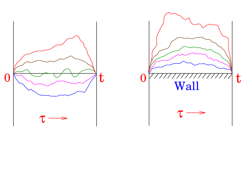
Figure 1: Typical watermelon configurations without a wall (left) and with a wall (right) at the origin for $N=5$ nonintersecting Brownian motions over the time interval $0\leq\tau\leq t$.

Recently, the transverse fluctuations of $N$ nonintersecting lines have been studied extensively in watermelon geometry over $[0,t]$ both with and without a wall and important connections to random matrix theory have been discovered Ferrari ; JohanssonRMT ; Katori3 ; Katori2 ; Katori1 ; T-W ; Schehr ; N Kobayashi . For example, the joint distribution of the positions of all the walkers at a fixed time $0\leq\tau\leq t$ for watermelons without a wall was shown to be identical (after appropriate rescaling) to the joint distribution of eigenvalues of a Gaussian random matrix belonging to the unitary (GUE) ensemble JohanssonRMT ; Katori1 . On the other hand, the joint distribution of the positions at a fixed time $0\leq\tau\leq t$ for watermelons with a hard wall at the origin was computed recently Schehr and was shown to be identical (after an appropriate change of variable) to the joint distribution of eigenvalues of a random matrix drawn from the Wishart (or Laguerre) ensemble at a special value of its parameters, which also corresponds to the chiral Gaussian unitary ensemble of random matrices Katori2 .

It is useful at this point to recollect the definition of a Wishart matrix. A Wishart matrix $W$ is an $(N\times N)$ square matrix of the product form $W=X^{\dagger}X$ where $X$ is a $(M\times N)$ rectangular matrix with real or complex entries and $X^{\dagger}$ is its Hermitian conjugate. If the entries $X_{ij}$ represent some data, e.g., $X_{ij}$ may indicate the price of the $j$-th commodity on the $i$-th day, then $W$ is just the (unnormalized) covariance matrix that provides informations about the correlations between prices of different commodities. If $X$ is a Gaussian random matrix, $P(X)\propto\exp\left[-\frac{\beta}{2}{\rm Tr}(X^{\dagger}X)\right]$ where the Dyson index $\beta=1,2$ corresponds respectively to real and complex matrices, then the random covariance matrix $W$ belongs to the Wishart ensemble named after Wishart who introduced them in the context of multivariate statistical data analysis Wishart . Since then the Wishart matrix has found numerous applications. Wishart matrices play an important role in data compression techniques such as the “Principal Components Analysis” (PCA). PCA applications include image processing Wilks ; Fukunaga ; Smith , biological microarrays arrays1 ; arrays2 , population genetics Cavalli ; Patterson ; genetics , finance BP ; Burda , meteorology and oceanography Preisendorfer . The spectral properties of the Wishart matrices have been studied extensively and it is known James that for $M\geq N$, all $N$ positive eigenvalues of $W$ are distributed via the joint probability density function (pdf)

$$P_{N}(\lambda_{1},...,\lambda_{N})=K_{N}\,e^{-\frac{\beta}{2}\,\sum_{k}\lambda_{k}}\prod_{k=1}^{N}\lambda_{k}^{\frac{\beta}{2}(M-N+1)-1}\,\prod_{i<j}|\lambda_{i}-\lambda_{j}|^{\beta}$$ (1)

where $K_{N}$ is a normalization constant and the Dyson index $\beta=1,2$ (respectively for real and complex $X$). In the “Anti-Wishart” case, that is when $M<N$, $W$ has $M$ positive eigenvalues ( and $N-M$ eigenvalues that are exactly zero ) and their joint probability distribution is simply obtained by exchanging $M$ and $N$ in the formula (1). Hence we will focus only on the Wishart case with $M\geq N$. Note that even though the Wishart pdf in Eq. (1) was obtained for integer $M\geq N$, the pdf is actually a valid measure for any real continuous $M\geq N$. In particular, for $M-N=\frac{1}{2}$ ($M-N=-\frac{1}{2}$) in the case $\beta=2$, the pdf in Eq. (1) is realized as the distribution of the squares of positive eigenvalues of class $C$ ($D$) random matrices Katori2 , in the classification of Altland and Zirnbauer Altland . In addition, the pdf in Eq. (1) is also realized for $d$-dimensional squared Bessel processes under nonintersection constraint with $\beta=2$ and $M-N=d/2-1$ for $d>0$ Katori4 .

In Ref. Schehr , the joint pdf of the positions of $N$ nonintersecting Brownian motions in the ‘watermelon with a wall’ geometry, mentioned in the previous paragraph, was shown to correspond to the joint pdf of Wishart ensemble in Eq. (1) with special values of the parameter $\beta=2$ and $M-N=1/2$. At these special values, the joint pdf also correspond to those of the squares of the eigenvalues of class $C$ matrices Katori2 . A question thus naturally arises whether it is possible to find a nonintersecting Brownian motion model that will generate a Wishart ensemble in Eq. (1) with arbitrary values of the two parameters $\beta$ and $M-N\geq 0$. In this paper we address precisely this issue and show how to generate the Wishart ensemble with arbitrary positive $\beta$ and $M-N\geq 0$, starting from an underlying microscopic model of nonintersecting Brownian motions.

In this paper we study the nonintersecting Brownian motions in a geometry different from that of the watermelons discussed above. Here we consider a system of $N$ $(1+1)$-dimensional nonintersecting fluctuating elastic interfaces with heights $h_{i}(x)$ ($i=1,2,3,\dots N)$ that run across the interval $x\in[0,L]$ in the longitudinal direction (see Fig. 2). Equivalently the heights $\{h_{i}(x)\}$ can be thought of as the positions of $N$ nonintersecting walkers at ‘time’ $x$. In contrast to the watermelon geometry, the lines here are not constrained to reunite at the two end points. Instead, each line satisfies the periodic boundary condition in the longitudinal direction, i.e., they are wrapped around a cylinder of perimeter $L$ (see Fig. 2). In addition, there is a hard wall (or substrate) at $h=0$ that induces an external confining potential $V(h_{i})$ on the $i$-th interface for all $1\leq i\leq N$. In a slightly more general version of the model, one can also introduce a pairwise repulsive interaction between lines. In presence of the external confining potential $V(h_{i})$, the system of elastic lines reaches a thermal equilibrium and our main goal is to compute the statistical properties of the heights of these lines at thermal equilibrium. More precisely, we compute the joint distribution of heights of the lines at a fixed position $0\leq x\leq L$ and show that, in the limit $L\rightarrow\infty$ (large system), this joint distribution, after an appropriate change of variables, is precisely the same as the joint distribution in the Wishart ensemble. Note that due to the translational symmetry in the longitudinal direction (imposed by the periodic boundary condition), this joint pdf of the heights is actually independent of $x$.

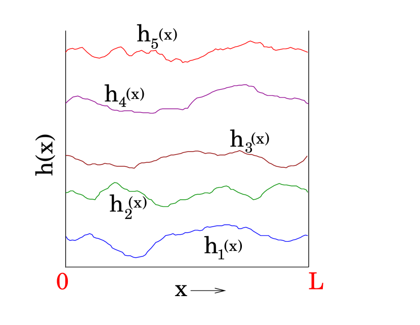
Figure 2: Nonintersecting fluctuating interfaces with heights $h_{i}(x)$ for $0\leq x\leq L$ with periodic boundary conditions, $h_{i}(0)=h_{i}(L)$.

Thus our model is actually closer to the solid-on-solid (SOS) models at thermal equilibrium in presence of a substrate Forgacs , except with the difference that here we have multiple nonintersecting interfaces. This model is thus appropriate to describe the interfaces between different co-existing ‘wet’ phases of a multiphase two-dimensional fluid system on a solid substrate or a film fisher . We note that nonintersecting Brownian motions in an external harmonic potential was studied recently by Bray and Winkler Bray , but they were mostly interested in calculating the probability that such walkers all survive up to some time $t$. In the Brownian motion language, we are here interested in a different question: given that each walker survives up to ‘time’ $L$ and comes back to its starting position, what is the joint distribution of the positions of the walkers (or equivalently the heights of the interfaces) at any intermediate ‘time’ $0\leq x\leq L$ ?

In this paper, we consider the external confining potential of the form

$$V(h)=\frac{b^{2}h^{2}}{2}+\frac{\alpha(\alpha-1)}{2h^{2}}\;\;\textrm{with}\;\;b>0\;\;\textrm{and}\;\;\alpha>1$$ (2)

with a harmonic confining part and a repulsive inverse square interaction. Such a choice is dictated by the following observations. The harmonic potential is needed to confine the interfaces as otherwise there will be a zero mode. The repulsive inverse square potential has an entropic origin. For a single interface near a hard wall, Fisher fisher indeed showed that the effective free energy at temperature $T$ behaves as $k_{B}T/h^{2}$ where $h$ is the distance of the interface (or the walker) from the wall. Thus it is natural to choose the external potential of the form as in Eq. (2). In addition, as we will see later, such a physical choice also has the advantage that it is exactly soluble. We will see indeed that this choice of the potential generates, for the joint density of heights at a fixed point $x$ and in the limit of a large system ($L\rightarrow\infty$), a Wishart pdf in Eq. (1) with fixed $\beta=2$, but with a tunable $M-N=\alpha-1/2$ where $\alpha$ sets the amplitude of the repulsive inverse square potential in Eq. (2). Thus when $\alpha-1/2=k$ is a positive integer $k$, this generates a physical realization of Wishart matrices with integer dimensions $M=N+k$ and $N$.

Our model is also rather close to the realistic experimental system of fluctuating step edges on vicinal surfaces of a crystal in presence of a substrate (or hard wall). When a crystal is cut by a plane which is oriented at a small nonzero angle to the high-symmetry axis, one sees a sequence of terraces oriented in the high-symmetry direction that are separated by step edges which can be modelled as ‘elastic’ nonintersecting lines or trajectories of nonintersecting Brownian motions Einstein . In an external confining harmonic potential but in absence of a wall at $h=0$ (such that $h\to-h$ symmetry is preserved), the joint distribution of the heights of the lines at equilibrium can be mapped to the GUE ensemble Einstein , although most studies in this context are concerned with the so called Terrace-Width distribution, i.e., the distribution of the spacings between the lines. In our model, due to the presence of the wall which breaks the $h\to-h$ symmetry, new interesting questions emerge. For example, it is natural also to ask for the distribution of the minimal (maximal) height, i.e., the height of the line closest (farthest) from the wall. Using the mapping to the Wishart random matrix, the minimal and maximal height correspond respectively to the smallest and the largest eigenvalue of the Wishart random matrix. In addition, it is also interesting and physically relevant to investigate the statistics of the center of mass of the $N$ nonintersecting Brownian motions. We will see that strong correlations between the lines violate the central limit theorem resulting in strong non-Gaussian tails in the distribution of the center of mass.

Let us summarize below our main results.

$\bullet$ Using a path integral formalism we show that the computation of the equilibrium joint distribution of heights at a fixed point in space can be mapped to determining the spectral properties of a quantum Hamiltonian. Subsequently, when the external potential is of the form in Eq. (2), this quantum potential turns out to be integrable and allows us to compute the equilibrium joint distribution of heights exactly. In particular in the limit of a large system ($L\rightarrow\infty$), we show that the joint distribution of heights, under a change of variables $b\,h_{i}^{2}=\lambda_{i}$, is exactly of the Wishart form in Eq. (1) with parameters $\beta=2$ and $M-N=\alpha-1/2$ where $\alpha$ appears in the potential in Eq. (2). Knowing the exact joint distribution, we then compute various statistical properties of the heights of the interfaces as listed below.

$\bullet$ We find that the average density of lines at height $h$, in the limit of a large number $N$ of interfaces, is a quarter of ellipse as a function of $h$, with finite support over $[0,2\sqrt{\frac{N}{b}}]$ where $b$ appears in Eq. (2). The typical height thus scales with $N$ for large $N$ as $h_{\rm typ}\sim\sqrt{N}$. This differs considerably from the case of $N$ interfaces that are allowed to cross, where the typical height is of order one. The spreading of nonintersecting interfaces is a consequence of the strong interaction between them induced by their fermionic repulsion.

$\bullet$ We study the height distribution of the topmost (farthest from the wall) interface in the large $N$ limit. We show that the average height of the farthest interface (maximal height) is $2\sqrt{\frac{N}{b}}$ for large $N$ : it is given by the upper bound of the average density of states. The typical fluctuations of the maximal height around its mean are distributed via the Tracy-Widom distribution Johansson ; Johnstone ; T-W mean . However, for finite but large $N$, the tails of the distribution of the maximal height show significant deviations from the Tracy-Widom behavior. We compute exactly these large deviation tails.

$\bullet$ We also study the statistics of the height of the lowest (closest to the wall) interface (minimal height) and argue that, for large $N$, it scales as $N^{-1/2}$. This should be compared to the case of non-interacting Brownian motions where the typical distance of the closest (to the wall) walker is of $\sim O(1)$ from the wall. This is again an effect of the strong interaction between the interfaces: their mutual repulsion pushes the lowest interface closer to the substrate. We further show that the full distribution of the minimal height can be exactly computed for a special value of the parameter $\alpha=3/2$ in Eq. (2).

$\bullet$ Finally we study the distribution of the center of mass of the heights $G_{N}=\frac{h_{1}+...+h_{N}}{N}$ for large $N$. Thanks to the analogy between the Wishart eigenvalues and a Coulomb gas of charges, the mean and variance of the center of mass can be computed, as well as the shape of the probability distribution: we show that the pdf of $G_{N}$, $P(G_{N}=\nu)$, has a non-analytic behavior (essential singularity) at $\nu=\langle G_{N}\rangle$ (which is shown to be a direct consequence of a phase transition of ‘inifinite’ order in the associated Coulomb gas problem). In addition, we find exact asymptotic results, to leading order for large $N$, for the mean $\langle G_{N}\rangle=\frac{8}{3\pi}\sqrt{\frac{N}{b}}$ and the variance $\langle G_{N}^{2}\rangle-\langle G_{N}\rangle^{2}=\frac{2}{\pi^{2}Nb}$.

The rest of the paper is organized as follows. In section II, we present our model, compute (via path integral method) the joint probability distribution of the heights of the interfaces and compare it to the probability distribution of the eigenvalues of a Wishart matrix. In section III, we analyse some statistical properties of the model. We first present the results for the average density of lines (subsection III.1). We then compute the behavior of the maximal height (III.2) and the minimal height (III.3). Finally we study the distribution of the center of mass of the heights in (III.4). Section IV concludes the paper with a summary and outlook.

II The model

Our model consists of $N$ nonintersecting $(1+1)$-dimensional interfaces over a substrate of size $L$ (that induces an external potential). For simplicity, we first present the model for a single interface in subsection II.1 and show how, using a path-integral formalism, one can map the problem of calculating the equilibrium height distribution of the interface to computing the spectral properties of a quantum Hamiltonian. In particular, calculating the height distribution in the limit $L\rightarrow\infty$ (large system) corresponds to calculating the ground state wavefunction of this quantum Hamiltonian. Then we present the interacting model for general $N$ interfaces in subsection II.2 and show how to generalize the path integral formalism to a many-body problem and subsequently compute the joint distribution of heights at equilibrium. In particular, for a large system, the joint distribution is shown to have the Wishart form in Eq. (1) with parameters $\beta=2$ and $M-N=\alpha-1/2$ where $\alpha$ appears in the potential in Eq. (2).

II.1 One interface

Let us first consider the case of one single interface ($N=1$). The interface is described by its height $h(x)$ for $x$ from $0$ to $L$. When we think of the interface as a walker (or Brownian motion), the height $h$ plays the role of the position of the walker, while the coordinate $x$ along the substrate corresponds to time. The substrate can then be seen as a wall at height zero: one has $h(x)>0$ for every $x$. In the stationary state at thermal equilibrium, the energy of a configuration $\{h(x)\}$ of the interface can be expressed as

$$E\big{[}\{h(x)\}\big{]}=E_{elast}\big{[}\{h(x)\}\big{]}+U\big{[}\{h(x)\}\big{]}$$ (3)

with $E_{elast}\big{[}\{h(x)\}\big{]}=\frac{1}{2}\int_{0}^{L}dx\,\Big{(}\frac{dh}{dx}\Big{)}^{2}$ being the elastic energy (or the kinetic energy of the walker) and $U\big{[}\{h(x)\}\big{]}=\int_{0}^{L}dx\,V(h(x))$ describes the potential energy due to the interaction potential $V(h)$ with the substrate. The statistical weight of a configuration $[\{h(x)\},\,0\leq x\leq L]$ of the interface is thus simply (setting $k_{B}T=1$ where $k_{B}$ is the Boltzmann constant and $T$ the temperature) given by the Boltzmann weight

$$P\left[\{h(x)\}\right]\propto\exp\big{\{}-E\big{[}\{h(x)\}\big{]}\big{\}}\propto\exp\left\{-\frac{1}{2}\int_{0}^{L}\Big{(}\frac{dh}{dx}\Big{)}^{2}dx-\int_{0}^{L}V\left(h(x)\right)dx\right\}$$ (4)

We assume periodic boundary conditions: $h(0)=h(L)=h>0$.

In absence of an external potential ($V\equiv 0$), the interface is depinned, with a roughness exponent $\chi=1/2$, which means $\langle h^{2}\rangle-\langle h\rangle^{2}\propto L^{2\chi}\propto L$. In this case the interface is just the trajectory of a free one dimensional Brownian motion: the displacement $h$ of the walker grows as the square root of the ‘time’ ($L$). But when the substrate induces an attractive potential, the interface remains pinned to the wall (substrate). The interface then becomes smooth ($\chi=0$) in this case.

Given the overall statistical weight of the full configuration of an interface in Eq. (4) over $x\in[0,L]$, our task next is to compute the ‘marginal’ height distribution $P(h)$ of the interface at a fixed point $x$ in space, by integrating out the heights at other points. Note that due to the translational symmetry imposed by the periodic boundary condition, this marginal height distribution $P(h)$ is independent of the point $x$, which we can conveniently choose to be $x=0$ for example. This integration of all other heights except at $0$ (or $L$) can be very conveniently carried out by the following path integral that allows us to write the marginal pdf $P(h)$ as

$$P(h)\propto\int_{h(0)=h}^{h(L)=h}\mathcal{D}h(x)\>e^{-E\big{[}\{h(x)\}\big{]}}\,\,\mathbb{1}_{h(x)>0}$$ (5)

where the symbol $\mathbb{1}_{h(x)>0}$ is an indicator function that enforces the condition that the height at all points $x\in[0,L]$ is positive and the energy $E\big{[}\{h(x)\}\big{]}$ is given in Eq. (4).

The path integral can be reinterpreted as a quantum propagator:

$$P(h)\propto\langle h|e^{-\hat{H}L}|h\rangle$$ (6)

with the Hamiltonian

$$\hat{H}=-\frac{1}{2}\frac{d^{2}}{dh^{2}}+V(h)$$ (7)

and with the constraint $h>0$. The problem is now the one of a quantum particle in one dimension with position $h(x)$ at time $x$, described by the Hamiltonian $\hat{H}$ (in imaginary time).

We assume now that the energy spectrum of $\hat{H}$ is discrete (this will be the case in presence of the confining potential). The propagator can be decomposed in the eigenbasis of $\hat{H}$:

$$P(h)=\frac{\sum_{E}e^{-EL}\>\left|\psi_{E}(h)\right|^{2}}{\sum_{E}e^{-EL}}$$ (8)

where $\psi_{E}$ is the eigenfunction of energy $E$. Thus calculating the marginal height distribution is equivalent, thanks to the relation in Eq. (8), to calculating the full spectral properties (i.e., all eigenvalues and eigenfunctions) of the quantum Hamiltonian $\hat{H}$. In Eq. (6) and (8), the size $L$ of the substrate (in the classical system of interfaces) plays the role of the inverse temperature in the associated quantum problem (but it has nothing to do with the temperature of the interfaces). Hence, in a large system $L\to\infty$, only the ground state ($\psi_{E_{0}}\equiv\psi_{0}$ with energy $E_{0}$) contributes to the sum in Eq. (8). Henceforth, we will always work in this limit where the marginal pdf is given by the exact formula

$$P(h)=|\psi_{0}(h)|^{2}$$ (9)

Let us make a quick remark here. While the results in Eqs. (8) and (9) may apriori look evident, they are however a bit more subtle. For example, the r.h.s. of Eq. (9) is, in a quantum mechanical sense, the probability density of finding a particle at $h$ in the ground state. But it is not obvious (and needs to be proved as done above) that it also represents the height distribution of a classical model.

Thus our task is now to determine the exact ground state of the quantum Hamiltonian $\hat{H}$. Analytically this is only possible for integrable $\hat{H}$. With the choice of potential $V(h)$ as in Eq. (2), the quantum Hamiltonian $\hat{H}$ is fortunately integrable. The eigenfunction $\psi_{n}(h)$ satisfies the Schrödinger equation:

$$\hat{H}\psi_{n}=-\frac{1}{2}\frac{d^{2}\psi_{n}}{dh^{2}}+V(h)\psi_{n}=E_{n}\psi_{n}$$ (10)

with the boundary conditions, $\psi_{n}(h=0)=0$ (due to the hard wall at $h=0$) and $\psi_{n}(h\to\infty)=0$. The solution is of the form

$$\psi_{n}(h)=c_{n}\>e^{-\frac{b}{2}h^{2}}\;h^{\alpha}\;\mathcal{L}_{n}^{(\alpha-\frac{1}{2})}(bh^{2});\quad\quad\textrm{with}\>\;\;E_{n}=b\,(2n+\alpha+\frac{1}{2})$$ (11)

with $n$ a non-negative integer (discrete spectrum), $c_{n}$ a normalization constant and $\mathcal{L}_{n}^{(\alpha-\frac{1}{2})}$ a generalized Laguerre polynomial of degree $n$

$$\mathcal{L}_{n}^{\gamma}(x)=\sum_{i=0}^{n}\left(\begin{array}[]{c}n+\gamma\\ n-i\end{array}\right)\,\frac{(-x)^{i}}{i!}$$ (12)

Note that for $\gamma=0$, $\mathcal{L}_{n}^{0}(x)=\mathcal{L}_{n}(x)$ reduces to the ordinary Laguerre polynomial

$$\mathcal{L}_{n}(x)=\sum_{i=0}^{n}\left(\begin{array}[]{c}n\\ i\end{array}\right)\,\frac{(-x)^{i}}{i!}.$$ (13)

We also note that the generalized Laguerre polynomial in Eq. (12) can alternately be expressed as a hypergeometric function

$$\mathcal{L}_{n}^{\gamma}(x)=\frac{(\gamma+1)_{n}}{n!}\,_{1}F_{1}(-n;\gamma+1;x).$$ (14)

where $(a)_{n}=(a)(a+1)...(a+n-1)$ is the Pochhammer symbol and

$${}_{p}F_{q}(a_{1},...,a_{p};b_{1},...,b_{q};z)=\sum_{n=0}^{\infty}\frac{(a_{1})_{n}...(a_{p})_{n}}{(b_{1})_{n}...(b_{q})_{n}}\frac{z^{n}}{n!}.$$ (15)

Finally, as $\mathcal{L}_{0}^{\gamma}(x)=1$, the pdf of the height of the interface is (in the limit of a large substrate $L\rightarrow\infty$)

$$P(h)=|\psi_{0}(h)|^{2}=|c_{0}|^{2}\,\>e^{-b\,h^{2}}\;h^{2\alpha}$$ (16)

with $|c_{0}|^{2}=\frac{2\,b^{\alpha+1/2}}{\Gamma(\alpha+1/2)}$.

The mean $m\equiv\langle h\rangle$ and variance $\sigma_{1}^{2}\equiv{\rm Var}(h)=\langle h^{2}\rangle-\langle h\rangle^{2}$ of the interface height are thus easy to compute:

$$m=\langle h\rangle=\int_{0}^{\infty}dh\,h\,P(h)=\frac{\Gamma(\alpha+1)}{\sqrt{b}\;\,\Gamma(\alpha+1/2)}$$ (17)

$$\sigma_{1}^{2}={\rm Var}(h)=\frac{1+2\alpha}{2\,b}-\frac{1}{b}\,\left(\frac{\Gamma(\alpha+1)}{\Gamma(\alpha+1/2)}\right)^{2}$$ (18)

II.2 $N$ interfaces

Let us consider now $N$ nonintersecting $(1+1)$-dimensional interfaces over a substrate of size $L$. The $i^{th}$ interface is described by its height $h_{i}(x)$ for $x$ from $0$ to $L$. Since the interfaces are nonintersecting, we can assume that they are ordered: $0<h_{1}(x)<h_{2}(x)<...<h_{N}(x)$ for every $x$. The only interaction between the interfaces is their fermionic repulsion (they do not cross). However, we will see that this constraint drastically changes the statistics of the interfaces. In the stationary state (at thermal equilibrium), the energy $E\big{[}\{h(x)\}\big{]}$ of a configuration $\{h(x)\}$ of one of the interfaces is given by (3) (same form as we assumed for one single interface), with an elastic energy and a potential $V(h)$ again given by (2). Therefore the statistical weight of a configuration $\{h_{i}(x)\,;1\leq i\leq N,\>0\leq x\leq L\}$ of the whole system is simply (setting $k_{B}T=1$ for simplicity):

$$P\left[\{h_{i}(x)\}_{i,x}\right]\propto\exp\left[-\sum_{i}\frac{1}{2}\int_{0}^{L}\Big{(}\frac{dh_{i}}{dx}\Big{)}^{2}dx-\sum_{i}\int_{0}^{L}V\left(h_{i}(x)\right)dx\right]$$ (19)

We assume again periodic boundary conditions: for every $i$, $h_{i}(0)=h_{i}(L)=h_{i}$ with $0<h_{1}<h_{2}<...<h_{N}$. The configuration space can thus be seen as a cylinder of radius $L/2\pi$.

The joint probability distribution of the heights of the interfaces at a given position (position $x$ that can be taken to be $0$ by cylindrical symmetry, as we already noticed) can again be expressed as a path integral:

$$P(h_{1},h_{2},...,h_{N})\propto\prod_{i}\int_{h_{i}(0)=h_{i}}^{h_{i}(L)=h_{i}}\mathcal{D}h_{i}(x)\>e^{-\sum_{i}E\big{[}\{h_{i}(x)\}\big{]}}\>\mathbb{1}_{h_{N}(x)>...>h_{1}(x)>0}$$ (20)

The path integral can then be reinterpreted as a quantum propagator for $N$ particles:

$$P(h_{1},h_{2},...,h_{N})\propto\langle h_{1},h_{2},...,h_{N}|e^{-\hat{H}L}|h_{1},h_{2},...,h_{N}\rangle$$ (21)

where the many-body Hamiltonian is given by

$$\textrm{with }\>\;\hat{H}=\sum_{i}\hat{H}_{i}=-\sum_{i}\frac{1}{2}\frac{d^{2}}{dh_{i}^{2}}+\sum_{i}V(h_{i})$$ (22)

with the constraint $h_{N}>...>h_{1}>0$. The problem is now the one of $N$ independent fermionic particles in one dimension with positions $h_{i}(x)$ at time $x$, described by the single particle Hamiltonian $\hat{H}_{i}$ (in imaginary time).

Exactly as for one single interface, the propagator can be decomposed in the eigenbasis of $\hat{H}$ (Hamiltonian for $N$ particles) and the joint distribution of heights is given by

$$P(h_{1},h_{2},\ldots,h_{N})=\frac{\sum_{E}e^{-EL}\>\left|\psi_{E}(h_{1},h_{2},\ldots,h_{N})\right|^{2}}{\sum_{E}e^{-EL}}$$ (23)

where $\psi_{E}(h_{1},h_{2},\ldots,h_{N})$ is the many-body wavefunction at energy $E$. Analogus to the single interface case, when the size of the system $L$ tends to infinity, only the ground state $\Psi_{0}$ ($N$-body wavefunction) contributes to the sum. In this limit, the joint probability is simply:

$$P(h_{1},h_{2},...,h_{N})=|\Psi_{0}(h_{1},...,h_{N})|^{2}$$ (24)

As in the single particle case, we emphasise that the relations in Eqs. (23) and (24) may apriori look evident, but they need to be proved as the l.h.s and r.h.s. of these equations refer to the probability density in a classical and a quantum problem respectively. We note that in the context of step edges on vicinal surfaces (in the absence of a wall), the relation (24) was implicitly assumed in Ref. Einstein , but not proved.

In the case of one interface, we computed the single particle wavefunction $\psi_{n}$ in (11). As the particles are independent fermions, the ($N$-body) ground state wavefunction $\Psi_{0}$ is a $N\times N$ Slater determinant. It is constructed from the $N$ single particle wavefunctions of lowest energy, the $\psi_{i}$ for $i$ from $0$ to $N-1:$

$$\Psi_{0}(h_{1},...,h_{N})\propto\det\left(\psi_{i-1}(h_{j})\right)\propto e^{-\frac{b}{2}\sum_{k}h_{k}^{2}}\;\prod_{k}h_{k}^{\alpha}\;\>\det\left(\mathcal{L}_{i-1}^{(\alpha-\frac{1}{2})}(bh_{j}^{2})\right)$$ (25)

Note that $\mathcal{L}_{i-1}^{(\alpha-\frac{1}{2})}(bh^{2})$ is a polynomial of $h^{2}$ of degree $i-1$. Any determinant involving polynomials can be reduced, via the linear combination of rows, to a Vandermonde determinant which can then be simply evaluated. We then get

$$P(h_{1},...,h_{N})=|\Psi_{0}(h_{1},...,h_{N})|^{2}\,\propto e^{-b\sum_{k}h_{k}^{2}}\;\prod_{k}h_{k}^{2\alpha}\;\>\prod_{i<j}(h_{i}^{2}-h_{j}^{2})^{2}$$ (26)

where $h_{i}$’s are positive. Note that due to the symmetry of the above expression, the ordering constraint $h_{1}<...<h_{N}$ can be removed by simply dividing the normalization constant by $N!$.

For interfaces that are allowed to cross, the joint probability distribution of the heights has a similar form, but without the Vandermonde determinant: $P(h_{1},...,h_{N})=P(h_{1})...P(h_{N})\propto e^{-b\sum_{k}h_{k}^{2}}\;\prod_{k}h_{k}^{2\alpha}$. The Vandermonde determinant $\prod_{i<j}(h_{i}^{2}-h_{j}^{2})^{2}$ comes from the fermionic repulsion between the interfaces. In particular, one has (as expected) for nonintersecting interfaces $P(h_{1},...,h_{N})=0$ if $h_{i}=h_{j}$ for $i\neq j$. The consequence of this repulsion on the typical magnitude of the heights of interfaces will be explored in the next section.

II.3 Relation to the Eigenvalues of a Wishart Matrix

We recall from the introduction that an $(N\times N)$ Wishart matrix is a product covariance matrix of the form $W=X^{\dagger}X$ where $X$ is a Gaussian $(M\times N)$ rectangular matrix drawn from the distribution, $P(X)\propto\exp\left[-\frac{\beta}{2}{\rm Tr}(X^{\dagger}X)\right]$. For $M\geq N$, all eigenvalues of $W$ are non-negative and are distributed via the joint pdf in Eq. (1). In the “Anti-Wishart” case, that is when $M<N$, $W$ has $M$ positive eigenvalues ( and $N-M$ eigenvalues that are exactly zero ) and their joint probability distribution is simply obtained by exchanging $M$ and $N$ in the formula (1).

The joint probability distribution of the heights of the interfaces in our model in Eq. (26) can then be related to the Wishart pdf in Eq. (1) with $\beta=2$ after a change of variables $b\,h_{i}^{2}=\lambda_{i}$

$$P(h_{1},\ldots,h_{N})dh_{1}...dh_{N} \propto e^{-b\sum_{k}h_{k}^{2}}\;\prod_{k}h_{k}^{2\alpha}\;\>\prod_{i<j}(h_{i}^{2}-h_{j}^{2})^{2}dh_{1}\ldots dh_{N}$$ (27)

$$=A_{N}\,e^{-\sum_{k}\lambda_{k}}\;\prod_{k}\lambda_{k}^{\alpha-\frac{1}{2}}\;\>\prod_{i<j}(\lambda_{i}-\lambda_{j})^{2}d\lambda_{1}\ldots d\lambda_{N}$$

where $A_{N}$ is a normalization constant. Recall that the parameter $\alpha>1$. By choosing $\alpha=(M-N)+\frac{1}{2}>1$, one recovers the Wishart pdf in Eq. (1) for $\beta=2$ (complex matrices $X$) and arbitrary $M-N>1/2$. Thus by tuning the amplitude $\alpha$ of the repulsive part of the potential in Eq. (2) one can generate the Wishart ensemble with a tunable $M$ (with $M-N>1/2$). The normalization constant $A_{N}$ can be computed using Selberg’s integrals Mehta and one gets

$$A_{N}^{-1}=\prod_{k=1}^{N}\left(k!\,\>\Gamma(\alpha-\frac{1}{2}+k)\right)$$ (28)

Wishart pdf with arbitrary $\beta\geq 0$ and $M>N$: We note that our model above generates a Wishart pdf with arbitrary $M-N>1/2$ but with fixed $\beta=2$. It is possible to generate the Wishart pdf with arbitrary $\beta\geq 0$ also by introducing an additional pairwise repulsive potential between the interfaces. For example, we may add to the energy functional in Eq. (19) an additional pairwise interaction term of the form,

$$-\sum_{1\leq j<k\leq N}\,\int_{0}^{L}V_{\rm pair}\left(h_{j}(x),\,h_{k}(x)\right)\,dx$$ (29)

where the pair potential $V_{\rm pair}(h_{j},h_{k})$ has a specific form

$$V_{\rm pair}(h_{j},h_{k})=\frac{\beta}{2}\,\left(\frac{\beta}{2}-1\right)\,\left[\frac{1}{(h_{j}-h_{k})^{2}}+\frac{1}{(h_{j}+h_{k})^{2}}\right]$$ (30)

with $\beta\geq 0$. In this case, once again using the path integral formalism developed above, we can map the computation of the joint distribution of heights to calculating the spectral properties of a quantum Hamiltonian via Eqs. (23) and (24). The corresponding quantum Hamiltonian turns out to be exactly the Calogero-Moser model Moser which is integrable OP ; YKY . In particular, using the exact ground state wavefunction of this Hamiltonian we get our corresponding joint distribution of interface heights in the following form

$$P(h_{1},...,h_{N})=|\Psi_{0}(h_{1},...,h_{N})|^{2}\propto e^{-b\sum_{k}h_{k}^{2}}\;\prod_{k}h_{k}^{2\alpha}\;\>\prod_{i<j}(h_{i}^{2}-h_{j}^{2})^{\beta}$$ (31)

which, after the usual change of variables $b\,h_{i}^{2}=\lambda_{i}$, corresponds to the general Wishart pdf in Eq. (1) with arbitrary $\beta\geq 0$ and a tunable $M-N=(2\alpha+1-\beta)/\beta$. We note that the procedure used above to obtain a variable $\beta$ random matrix ensemble was used before in the context of step edges on vicinal surfaces without a hard wall where a corresponding Gaussian matrix ensemble with tunable $\beta$ was obtained Einstein .

Note that for interfaces in presence of a wall, while the first term in the pair potential in Eq. (30) is quite natural and can arise out of entropic origin as well as dipolar interaction between step edges Einstein , the second term however does not have any physical origin. Unfortunately if one gets rid of this term, the integrability of the quantum Hamiltonian also gets lost. In any case, in the following we would focus only on the physical $\beta=2$ case.

III Statistical properties of the model

Once the joint distribution of heights at equilibrium is known, one can, at least in principle, compute the statistics of various relevant quantitites such as the average density of lines at height $h$, the distribution of the maximal and the minimal height, the distribution of the center of mass of the interfaces etc. In this section we show how to carry out this procedure and derive some explicit results upon borrowing the techniques developed in the context of random matrix theory. Many of the results in Secs. III A-C actually follow from a simple change of variables in the already known results of random matrix theory. For the sake of completeness, we remind the readers some of these results from random matrix theory and draw the consequences for our interface model. However, Sec. III D (where we derive the distribution of the center of mass of the interfaces) presents completely new results.

For simplicity, we will focus here only on large system ($L\rightarrow\infty$) properties. In particular, our focus would be to understand the effect of fermionic repulsion between the interfaces (nonintersecting constraint) and also the effect of the external confining potential on the statistics of the above mentioned physically relevant quantities.

We have shown in the previous section that the joint pdf of interface heights ($h_{i}$), after the change of variables $b\,h_{i}^{2}=\lambda_{i}$, is the same as the joint pdf of Wishart eigenvalues ($\lambda_{i}$) in Eq. (1), which can be re-written as a Boltzmann weight

$$P_{N}(\lambda_{1},...,\lambda_{N})\propto\exp\left[-\beta E_{\rm eff}(\lambda_{1},...,\lambda_{N})\right]$$ (32)

with the effective energy

$$E_{\rm eff}=\frac{1}{2}\,\sum_{k}\lambda_{k}-a\sum_{k}\ln\lambda_{k}-\sum_{i<j}\ln|\lambda_{i}-\lambda_{j}|$$ (33)

where $a=\left(\frac{1+M-N}{2}-\frac{1}{\beta}\right)$. In this form, the $\lambda_{i}$’s can be interpreted as the positions of charges repelling each other via the $2$-d Coulomb interaction (logarithmic), but are confined on the $1$-d positive axis and in presence of an external linear+logarithmic potential. The Dyson index $\beta$ plays the role of inverse temperature. Our model of interfaces corresponds to $\beta=2$ (see Eq. (27)).

We already noticed that the nonintersection constraint for the interfaces is equivalent to the presence of the Vandermonde determinant, and thus the logarithmic Coulomb repulsion, in the joint probability distribution. For independent interfaces (allowed to cross), there is no Vandermonde term and hence the logarithmic repulsion term in Eq. (33) is absent. In that case, balancing the first two terms of the energy gives a typical height of order one: $h_{\rm typ}\sim O(1)$. But for the nonintersecting case, when the number $N$ of interfaces becomes large, the logarithmic repulsion is stronger than the logarithmic part of the external potential (provided $a$ is not proportional to $N$). Therefore, balancing the first and the third term in the effective energy gives, for large $N$, $N\lambda_{\rm typ}\sim N^{2}$, thus $\lambda_{\rm typ}\sim N$ or equivalently $h_{\rm typ}\sim\sqrt{N}$. The effect of repulsion is strong: the interfaces spread out considerably.

Below we first compute the average density of states, followed by the computation of the distribution of the topmost interface (maximal height) and the lowest interface (minimal height) that is the closest to the substrate. Finally we analyze the distribution of the center of mass of the heights.

III.1 Average density of states

We would first like to know what fraction of $N$ interfaces lie, on an average, within a small interval of heights $[h,h+dh]$. This is given by the average density of states (normalized to unity)

$$\rho_{N}(h)=\frac{1}{N}\sum_{i=1}^{N}\langle\delta(h-h_{i})\rangle$$ (34)

As we explained above, we expect the typical height scale to be of order $h_{\rm typ}\sim\sqrt{N}$ for a large number $N$ of interfaces. Furthermore, the density of states is normalized to unity: $\int_{0}^{\infty}dh\>\rho_{N}(h)=1$. Therefore the density is expected to have the following scaling form for large $N$:

$$\rho_{N}(h)\approx\frac{1}{\sqrt{N}}\;\>g\left(\frac{h}{\sqrt{N}}\right)$$ (35)

Our goal is to compute this scaling function $g(x)$. This can actually be simply read off from the known results on Wishart matrices which we now recall. Consider the Wishart matrix with $M\geq N$ with eigenvalues distributed via the joint pdf in Eq. (1). In the asymptotic limit $N\to\infty$, $M\to\infty$ keeping the ratio $c=N/M$ fixed (with $c\leq 1$), the average density of states of the eigenvalues is known marcenko to be of the form:

$$\rho_{N}^{W}(\lambda)=\frac{1}{N}\sum_{i=1}^{N}\langle\delta(\lambda-\lambda_{i})\rangle\approx\frac{1}{N}f\left(\frac{\lambda}{N}\right)\;\;\textrm{for large $N$}$$ (36)

where the Marc̆enko-Pastur scaling function $f(x)$ depends on $c$ (but is independent of $\beta$)

$$f(x)=\frac{1}{2\pi x}\sqrt{(x_{+}-x)(x-x_{-})}$$ (37)

which has a non-zero support over the interval $x\in[x_{-},x_{+}]$ where $x_{\pm}=\left(\frac{1}{\sqrt{c}}\pm 1\right)^{2}$. Note that in the limit $c\to 1$, which happens when $M-N\sim O(1)$ for large $N$, $x_{-}\to 0$ and $x_{+}\to 4$.

Our interface model, after the customary change of variable $b\,h_{i}^{2}=\lambda_{i}$, corresponds to the Wishart ensemble in Eq. (1) with $\beta=2$ and $M-N=\alpha-1/2$. Hence, as long as $\alpha\sim O(1)$ for large $N$, $c=N/M\to 1$ in our model. Using $bh^{2}=\lambda$ and $c=1$ in Eq. (36) and (37), the average density of states in the interface model then indeed has the scaling form in Eq. (35) for large $N$ with the scaling function

$$g(x)=\frac{b}{\pi}\sqrt{\frac{4}{b}-x^{2}}$$ (38)

where $b$ is the frequency of the harmonic part of the potential (see (2)). The average density is a quarter of ellipse, as shown in figure 3. It has a finite support $\left[0\,,\,2\,\sqrt{\frac{N}{b}}\right]$.

Thus the interface heights spread out for large $N$ as a result of the nonintersection constraint. Let us compare this result to the case of independent interfaces that are allowed to cross each other. In that case, the average density of states is simply $\rho_{N}(h)=P(h)\propto e^{-b\,h^{2}}\;h^{2\alpha}$. It is independent of $N$ (evidently!) and has a non-zero support over the whole positive $h$ axis. It vanishes when $h$ tends to zero, and rapidly decreases to zero when $h$ becomes large. Thus most of the interfaces lie on an average close to the wall at a distance of $O(1)$. In contrast, the heights of nonintersecting interfaces, on an average for large $N$, have a compact support over a wide region. The density vanishes at the upper edge as a square root singularity and the upper edge itself grows as $\sqrt{N}$, thus spreading the interfaces further and further away from the wall as $N$ increases.

The average of the upper height (maximum) is expected to be given by the upper bound of the density support: $\langle h_{\rm max}\rangle\approx\>\,2\,\sqrt{\frac{N}{b}}$. The lower bound of the support of the density is zero for large $N$ in first approximation. We will show more precisely that the average height of the lower interface (minimum) is proportional to $\frac{1}{\sqrt{bN}}$.

Finally, the average of all interface heights $\langle h\rangle=\langle\frac{(h_{1}+h_{2}+\ldots+h_{N})}{N}\rangle$ can be computed for large $N$:

$$\langle h\rangle=\int_{0}^{\infty}h\rho_{N}(h)dh\approx\frac{8}{3\pi}\,\sqrt{\frac{N}{b}}$$ (39)

This differs drastically from the case of independent interfaces, where the average of all heights is the same as that for one single interface: $\langle h\rangle=\frac{\Gamma(\alpha+1)}{\sqrt{b}\;\,\Gamma(\alpha+1/2)}$ (see section II.1) is independent of $N$, but depends on $\alpha$ (parameter associated to the part of the potential proportional to $\frac{1}{h^{2}}$). In contrast, for nonintersecting interfaces, the part of the potential proportional to $\frac{1}{h^{2}}$ becomes negligible compared to the repulsion between interfaces, thus $\langle h\rangle$ does not depend on $\alpha$, but grows with $N$ (see (39)).

Figure 3: Rescaled average density of states $g(x)$ for the heights of interfaces plotted for $b=1$: $\rho_{N}(h)\approx\frac{1}{\sqrt{N}}\;\>g\left(\frac{h}{\sqrt{N}}\right)$. It is a quarter of ellipse.

III.2 Maximal height of the interfaces

In this subsection we compute the distribution of the height of the topmost interface (maximal height), the one furthest from the substrate. The average of the maximal height is given by the upper bound of the density support (see section III.1):

$$\langle h_{\rm max}\rangle\approx\>\,2\,\sqrt{\frac{N}{b}}\;\;\textrm{for large $N$.}$$ (40)

But we would like to know the full distribution of the height of the topmost interface, not just its average. For that purpose, we can again take advantage of the mapping between our interface model and the Wishart random matrix. Under this mapping, the height of the topmost interface $h_{\rm max}$ is related, via the change of variable $b\,h_{\rm max}^{2}=\lambda_{\rm max}$, to the largest eigenvalue $\lambda_{\rm max}$ of the Wishart matrix. The distribution of $\lambda_{\rm max}$ has been studied in great detail and we can then directly use these results for our purpose.

Let us recall briefly the known properties of the largest eigenvalue $\lambda_{\rm max}$ of Wishart matrices whose eigenvalues are distributed via the pdf in Eq. (1). For our purpose we will only focus on $\beta=2$ and $M\geq N$ with $M-N\sim O(1)$. In this case the parameter $c=N/M$ tends to the limiting value $c=1$ for large $N$, indicating that the upper edge of the Marc̆enko-Pastur sea, describing the average density of states in Eq. (37), approaches $x_{+}\to 4$ and lower edge $x_{-}\to 0$. Thus, the average of the maximal eigenvalue of a Wishart matrix is $\langle\lambda_{\rm max}\rangle\approx 4N$. Furthermore, Johansson Johansson and Johnstone Johnstone independently showed that the typical fluctuations of $\lambda_{\rm max}$ around its mean $4N$ are of order $N^{1/3}$, i.e.,

$$\lambda_{\rm max}\to 4N+2^{4/3}\,N^{1/3}\,\chi_{2}$$ (41)

where the random variable $\chi_{2}$ has an $N$-independent distribution for large $N$, ${\rm Prob}(\chi_{2}\leq x)=F_{2}(x)$ where $F_{2}(x)$ is the celebrated Tracy-Widom distribution T-W mean for $\beta=2$. However, for finite but large $N$, the tails of the pdf of $\lambda_{\rm max}$ (for $|\lambda_{\rm max}-4N|\sim O(N)$) show significant deviations from the Tracy-Widom behavior. The behavior in the tails of the pdf $P(\lambda_{\rm max}=t,N)$ is instead well described by the following functional forms Johansson , valid for arbitrary $\beta$,

$$P(t,N) \sim \exp\left[-\beta\,N^{2}\,\Phi_{-}\left(\frac{4N-t}{N}\right)\right]\quad{\rm for}\,\,t\ll 4N\,;$$ (42)

$$\sim \exp\left[-\beta\,N\,\Phi_{+}\left(\frac{t-4N}{N}\right)\right]\quad{\rm for}\,\,t\gg 4N\,;$$ (43)

where $\Phi_{\pm}(x)$ are the right (left) large deviation (rate) functions for the large positive (negative) fluctuations of $\lambda_{\rm max}$. Interestingly, the explicit form of the rate functions $\Phi_{\pm}(x)$ have recently been computed and were shown to be indepedent of $\beta$. The left rate function $\Phi_{-}(x)$ was computed in Ref. vivo using a Coulomb gas method developed in the context of Gaussian random matrices Dean and is given for $x\geq 0$ by

$$\Phi_{-}(x)=\ln\left(\frac{2}{\sqrt{4-x}}\right)-\frac{x}{8}-\frac{x^{2}}{64}.$$ (44)

The right rate function $\Phi_{+}(x)$ was also computed very recently vergassola using a different method

$$\Phi_{+}(x)=\frac{x+2}{2}-\ln(x+4)+\frac{1}{x+4}\,G\left(\frac{4}{4+x}\right)\,,$$ (45)

where $G(z)=_{3}F_{2}\left[\{1,1,3/2\},\{2,3\},z\right]$ is a hypergeometric function. For small argument $x$, the two rate functions have the following behavior vivo ; vergassola

$$\Phi_{-}(x) \approx x^{3}/{384}$$ (46)

$$\Phi_{+}(x) \approx x^{3/2}/6$$ (47)

Using these results, it was shown vivo ; vergassola that both large deviation tails of the pdf of $\lambda_{\rm max}$ in Eqs. (42) and (43) match smoothly with the inner Tracy-Widom form.

These results can then be directly translated to our problem of interfaces identifying $b\,h_{\rm max}^{2}=\lambda_{\rm max}$. For large $N$, the typical fluctuations of $h_{\rm max}$ around its mean are Tracy-Widom distributed (see figure 4) over a scale $\sim O(N^{-1/6})$. More precisely, we get

$$h_{\rm max}\approx 2\sqrt{\frac{N}{b}}+2^{-\frac{2}{3}}\,b^{-\frac{1}{2}}\>N^{-\frac{1}{6}}\,\chi_{2}$$ (48)

where $\chi_{2}$ is Tracy-Widom distributed, ${\rm Prob}(\chi_{2}\leq x)=F_{2}(x)$.

This gives in particular the first finite size correction to the leading term for the average of the maximal height, in the large $N$ limit:

$$\langle h_{\rm max}\rangle\approx 2\sqrt{\frac{N}{b}}+2^{-\frac{2}{3}}\,b^{-\frac{1}{2}}\>N^{-\frac{1}{6}}\,\langle\chi_{2}\rangle$$ (49)

where $\langle\chi_{2}\rangle\approx-1.7711$ T-W mean . The variance can also be computed from (48) and the known variance of the Tracy-Widom distribution $\langle\chi_{2}^{2}\rangle-\langle\chi_{2}\rangle^{2}\approx 0.8132$ T-W mean :

$${\rm Var}(h_{\rm max}) = \langle h_{\rm max}^{2}\rangle-\langle h_{\rm max}\rangle^{2}$$ (50)

$$\approx \frac{2^{-4/3}}{b}\,N^{-1/3}\left(\langle\chi_{2}^{2}\rangle-\langle\chi_{2}\rangle^{2}\right)$$

$$\approx \frac{0.32}{b\,N^{1/3}}$$

Figure 4: The dashed line shows the density of states $\rho_{N}(h)$ (quarter of ellipse). The height of the upper interface (maximal height) is centered around its mean $2\sqrt{\frac{N}{b}}$ with fluctuations of order $O(N^{-1/6})$ described by the Tracy-Widom law.

Similarly, the atypical large fluctuations of $h_{\rm max}$ around its mean (for $|h_{\rm max}-2\sqrt{N/b}|\sim O(N^{1/2})$) are described by the large deviation tails as for $\lambda_{\rm max}$ in Eqs. (42) and (43), with $\beta=2$. For the left large deviation, we get for $bt^{2}-4N\sim O(N)$ with $bt^{2}<4N$ :

$${\rm P}\left[h_{\rm max}=t,N\right]\approx\exp\left\{-2N^{2}\,\Phi_{-}\left(\frac{4N-bt^{2}}{N}\right)\right\}$$ (51)

where $\Phi_{-}(x)$ is given in Eq. (44).

Analogously the large and rare fluctuations to the right of the mean can also be computed from the exact expression of $\Phi_{+}(x)$ in Eq. (45). Replacing again $\lambda_{\rm max}$ by $b\,h_{\rm max}^{2}$, we get the right large deviation tail of the pdf of $h_{\rm max}$, for large $N$ and for $bt^{2}-4N\sim O(N)$ with $bt^{2}>4N$:

$${\rm P}\left[h_{\rm max}=t,N\right]\approx\exp\left\{-2N\,\Phi_{+}\left(\frac{bt^{2}-4N}{N}\right)\right\}$$ (52)

where $\Phi_{+}(x)$ is given in Eq. (45).

Figure 5: Pdf of the maximum of the heights (large deviation), plotted for $b=1$ and for different $N$, as a function of the rescaled height $x=\frac{t}{2\,\sqrt{N}}$. As $N$ increases, the rescaled location of the peak of the pdf approaches to $x\to 1$. The width of the regime around the peak where the Tracy-Widom law is valid is reduced to $\sim N^{-1/6-1/2}\sim N^{-2/3}$ in this scale. The rest of the pdf beyond the peak are described by the large deviation tails in Eqs. (51) and (52).

III.3 Minimal height of the interfaces

We have seen in subsection III.1 that the lower bound of the support of the average density of interfaces is indeed zero in the first approximation as $N\to\infty$. Since the lower edge of the support is also precisely the average height of the lowest (close to the substrate) interface, we have $\langle h_{\rm min}\rangle\to 0$ as $N\to\infty$. This is clearly an effect of the fermionic repulsion between the interfaces, because for ‘independent’ interfaces (that are allowed to cross) the height of the lowest interface (minimal height) is of order $h_{\rm min}\sim O(1)$: it does not see the other interfaces. The hard wall at the origin in the problem of interfaces corresponds to the constraint that the Wishart eigenvalues must be positive. In the Wishart ensemble, the neighborhood of the origin is, thus, called the hard edge of the spectrum. The distribution for the hard edge is known to be related to the Bessel kernel Forrester ; TWbis , just like the distribution at the soft edge (for the maximum eigenvalue) is related to the Airy kernel.

To know more precisely how $h_{\rm min}$ decreases with increasing $N$ in presence of the ‘nonintersection’ constraint, we need to find the statistics of $h_{\rm min}$ for large but finite $N$, which is precisely the objective of this subsection. The main result of this subsection is to show that for nonintersecting interfaces, the minimal height is typically of order $h_{\rm min}\sim O\left(\frac{1}{\sqrt{N}}\right)$ to leading order in large $N$. For special values of the parameters, we are also able to calculate the full distribution of the minimal height $h_{\rm min}$ as discussed below.

Under the customary change of variables $bh_{i}^{2}=\lambda_{i}$, it follows that $h_{\rm min}$ has the same distribution as $\sqrt{\lambda_{\rm min}/b}$ where $\lambda_{\rm min}$ is the minimum eigenvalue of Wishart ensemble with parameters $\beta=2$ and arbitrary $M\geq N$. The minimum eigenvalue of the Wishart ensemble has been studied before edelman , with applications in the quantum entanglement problem in bipartite systems majumdar-quant . When $M-N\sim O(1)$, which is precisely our case since $\alpha=M-N+1/2\sim O(1)$, the minimum eigenvalue is known to scale, for large $N$, as $\lambda_{\rm min}\sim 1/N$ for arbitrary $\beta$, though it has only been proved exactly for special values of $M-N$ and $\beta$, e.g., for $\beta=1$ and $M=N$ or for $\beta=2$ and $M=N$ edelman . For the interface model it then follows quite generally that $h_{\rm min}\sim 1/\sqrt{N}$ for large $N$ for general $\alpha\sim O(1)$. The fermionic repulsion between interfaces has thus again a strong effect: the lowest interface is pushed very close to the substrate since its height is of order $h_{\rm min}\sim 1/\sqrt{N}$ for large $N$ (instead of $O(1)$ for non-interacting interfaces that can cross).

To go beyond this scaling behavior for large $N$ and compute precisely the statistics of $h_{\rm min}$ for arbitrary $N$ seems difficult for general $\alpha$. Below we show that for the special case $\alpha=3/2$, it is possible to compute the full distribution of $h_{\rm min}$ for all $N$.

It turns out to be convenient to compute the cumulative distribution function (cdf) of the minimal height ${\rm Prob}\left[h_{\rm min}\geq\sqrt{\zeta},N\right]$, for arbitrary $\zeta$. We use the notation $\sqrt{\zeta}$ for the convenience of scaling as seen below. Our starting point is the central result for the joint pdf of interface heights in Eq. (26). Clearly, the event that the minimum height $h_{\rm min}\geq\sqrt{\zeta}$ is equivalent to the event that all the heights are greater than $\sqrt{\zeta}$: $h_{i}\geq\sqrt{\zeta}$ for all $i=1,2,\ldots,N$. Hence,

$${\rm Prob}\left[h_{\rm min}\geq\sqrt{\zeta},N\right]=\int_{\sqrt{\zeta}}^{\infty}dh_{1}\ldots\int_{\sqrt{\zeta}}^{\infty}dh_{N}\,P(h_{1},h_{2},\ldots,h_{N})$$ (53)

where the joint pdf $P(h_{1},h_{2},\ldots,h_{N})$ is given in Eq. (26). Making the standard change of variables, $bh_{i}^{2}=\lambda_{i}$ we then have

$${\rm Prob}\left[h_{\rm min}\geq\sqrt{\zeta},N\right]=A_{N}\int_{b\zeta}^{\infty}d\lambda_{1}\ldots\int_{b\zeta}^{\infty}d\lambda_{N}\>e^{-\sum_{k}\lambda_{k}}\;\prod_{k}\lambda_{k}^{\alpha-\frac{1}{2}}\;\>\prod_{i<j}(\lambda_{i}-\lambda_{j})^{2}$$ (54)

where the normalization constant $A_{N}$ is given in Eq. (28). Next, making a shift $\lambda_{i}=b\zeta+x_{i}$, one can rewrite Eq. (54) in a more compact form

$${\rm Prob}\left[h_{\rm min}\geq\sqrt{\zeta},N\right]=A_{N}\,e^{-bN\zeta}\,w(b\zeta)$$ (55)

where the function $w(z)$ is given by the multiple integral

$$w(z)=\int_{0}^{\infty}dx_{1}\ldots\int_{0}^{\infty}dx_{N}\;e^{-\sum_{k}x_{k}}\;\prod_{k=1}^{N}(x_{k}+z)^{\alpha-\frac{1}{2}}\;\>\prod_{i<j}(x_{i}-x_{j})^{2}.$$ (56)

For notational simplicity we have suppressed the $N$ and $\alpha$ dependence of $w(z)$. The multiple integral in Eq. (56) is not easy to evaluate for general values of the parameter $\alpha$. However, one can make progress for special values of $\alpha$.

We first note that when the parameter $\alpha-\frac{1}{2}=M-N$ is an integer, $w(z)$ is a polynomial of $z$ of degree $\alpha-\frac{1}{2}$. In the special case $\alpha=3/2$, i.e., $M=N+1$, one can explicitly evaluate $w(z)$ by following a method similar to the one used by Edelman edelman to compute the distribution of $\lambda_{\rm min}$ for Wishart matrices with $\beta=1$ and $M=N$. In this special case $M=N+1$ and $\beta=2$, the distribution of the minimum eigenvalue, in the large-$N$ limit, was already computed by Forrester Forrester . However, in this special case, one can actually calculate the distribution and the moments even for all finite $N$ as we demonstrate below. For $\alpha=3/2$ and $\beta=2$, we first compute two derivatives $w^{\prime}(z)$ and $w^{\prime\prime}(z)$ of the function $w(z)$ in Eq. (56). Using integration by parts and some rearrangements, we find that $w(z)$ satisfies an ordinary second order differential equation for any $N$

$$z\,w^{\prime\prime}(z)+(1+z)\,w^{\prime}(z)-N\,w(z)=0$$ (57)

whose unique (up to a constant) solution is in fact the ordinary Laguerre polynomial with negative argument

$$w(z)\propto\mathcal{L}_{N}(-z)=\sum_{k=0}^{N}\left(\begin{array}[]{c}N\\ k\end{array}\right)\frac{z^{k}}{k!}$$ (58)

and finally, since ${\rm Prob}\left[h_{\rm min}\geq 0,N\right]=1$, we get

$${\rm Prob}\left[h_{\rm min}\geq t,N\right]=e^{-bNt^{2}}\>\mathcal{L}_{N}(-b\,t^{2})=e^{-bNt^{2}}\>\sum_{k=0}^{N}\left(\begin{array}[]{c}N\\ k\end{array}\right)\,\frac{b^{k}\,t^{2k}}{k!}.$$ (59)

Hence, for the special case $\alpha=3/2$ we can then give an explicit expression for the pdf of $h_{\rm min}$ valid for all $N$,

$$P\left(h_{\rm min}=t,N\right)=-\frac{d}{dt}{\rm Prob}\left[h_{\rm min}\geq t,N\right]=2\,b^{2}\,t^{3}\,e^{-bNt^{2}}\>\mathcal{L}_{N-1}^{(2)}(-b\,t^{2})$$ (60)

where $\mathcal{L}_{n}^{\gamma}(x)$ is the generalized Laguerre polynomial already defined in Eq. (12).

From the exact pdf in Eq. (60) one can calculate all its moments explicitly as well (see appendix-A for details). We find for the $k$-th moment, for arbitrary $N$,

$$\langle h_{\rm min}^{k}\rangle=\frac{\Gamma(k/2+2)}{2b^{k/2}}\,\frac{(N+1)}{N^{k/2+1}}\,_{2}F_{1}\left(-(N-1),k/2+2;3;-1/N\right).$$ (61)

One can then work out the asymptotic behavior of the moments for large $N$. For example, one can show (see appendix-A) that the average value ($k=1$) $\langle h_{\rm min}\rangle$ decays for large $N$ as

$$\langle h_{\rm min}\rangle\approx\frac{c_{1}}{\sqrt{bN}}$$ (62)

with the constant prefactor $c_{1}$ given exactly by

$$c_{1}=\sqrt{\frac{\pi e}{4}}\,I_{0}(1/2)=1.5538\ldots$$ (63)

where $I_{n}(z)$ is the modified Bessel function of the first kind with index $n$

$$I_{n}(z)=\sum_{k=0}^{\infty}\frac{1}{k!\,(k+n)!}\left(\frac{z}{2}\right)^{2k+n}.$$ (64)

For large $N$, one can also work out precisely the scaling behavior of the full pdf of $h_{\rm min}$ given in Eq. (60) and recover the result of Forrester Forrester . Since typically $h_{\rm min}\sim 1/\sqrt{N}$, one expects that its pdf (normalized to unity) has a scaling form for large $N$

$$P\left(h_{\rm min}=t,N\right)\approx\sqrt{N}\,f_{\rm min}(t\,\sqrt{N}).$$ (65)

The scaling function $f_{\rm min}(x)$ can be computed explicitly from Eq. (60). We get

$$f_{\rm min}(x)=\lim_{N\rightarrow\infty}\frac{1}{\sqrt{N}}P\left(h_{\rm min}=\frac{x}{\sqrt{N}}\,,N\right)$$

$$\;\;\;\;\;=\lim_{N\rightarrow\infty}b^{2}\,x^{3}e^{-b\,x^{2}}\>\,_{1}F_{1}(1-N;3;\frac{bx^{2}}{N})$$

$$\;\;\;\;\;=\>b^{2}\,x^{3}\,e^{-b\,x^{2}}\,\,_{0}F_{1}(3;b\,x^{2})$$

$$\;\;\;\;\;=\>2b\,x\,e^{-b\,x^{2}}\>I_{2}(2x\sqrt{b}).$$ (66)

This function has the following asymptotic behavior

$$f_{\rm min}(x) \approx b^{2}\,x^{3}\quad{\rm as}\,\,x\to 0$$ (67)

$$\approx \frac{b^{3/4}}{\sqrt{\pi}}\,\sqrt{x}\,e^{-b\,x^{2}+2\,\sqrt{b}\,x}\quad{\rm as}\,\,x\to\infty$$

A plot of this scaling function is given in Fig. 6.

Figure 6: Rescaled probability density function of the minimum of the heights, in the case $\alpha=3/2$, plotted for $b=1$ and for $N=5$ (dashed line) and $N=20$ (dotted line) and compared with the limiting distribution $f_{\rm min}(x)$ (solid line). In the large $N$ limit, indeed the curves approach the limiting distribution $f_{\rm min}(x)$.

III.4 Center of mass

We study in this subsection the distribution of the center of mass of the heights

$$G_{N}=\frac{h_{1}+...+h_{N}}{N}$$ (68)

for large $N$. If the interfaces were allowed to cross, the heights $h_{i}$ would be independent and identically distributed variables (i.i.d.). In that case, the distribution of the center of mass $G_{N}$ would be a pure Gaussian distribution in the large $N$ limit (central limit theorem). But in our model, due to the repulsion between the interfaces, the interface heights are strongly correlated. What is the effect of the repulsion (nonintersecting constraint) on the center of mass? We will show how to compute the pdf of the center of mass for large $N$ upon borrowing some techniques developed in the context of random matrix theory, using in particular the analogy between the Wishart eigenvalues and a Coulomb gas of charges. We will show that the pdf of the center of mass $P(G_{N}=\nu)$ has an extraordinarily weak non-analytic behavior at $\nu=\langle G_{N}\rangle$ (where $\langle G_{N}\rangle$ is the average of the center of mass), which is shown to be a direct consequence of a phase transition in the associated Coulomb gas problem.

Since the typical height of an interface $h_{\rm typ}\sim\sqrt{N}$ for large $N$, it follows that the center of mass $G_{N}\approx O(\sqrt{N})$. More precisely, by symmetry of the joint pdf of the heights, the average of the center of mass is given by the average height (see (39)):

$$\langle G_{N}\rangle=\langle h\rangle\approx\frac{8}{3\pi}\,\sqrt{\frac{N}{b}}\equiv\mu\sqrt{N}\;\;\textrm{for large $N$,}\;\;\textrm{where}\;\;\mu=\frac{8}{3\pi\sqrt{b}}$$ (69)

Let us thus write $\nu=s\sqrt{N}$, where the scaled variable $s\sim O(1)$.

The main result of this subsection is to show that in the scaling limit $N\to\infty$, $\nu\to\infty$ but keeping the ratio $s=\nu/\sqrt{N}$ fixed, the pdf of the center of mass scales as:

$$P\left(G_{N}=\nu\right)\propto\exp\left[-N^{2}\>\Phi\left(\frac{\nu}{\sqrt{N}}\right)\right]$$ (70)

where the associated large deviation function $\Phi(s)$ is plotted in figure 8, has the following asymptotic behavior

$$\Phi(s)\approx\left\{\begin{array}[]{lcl}-2\ln s&{\rm for}&\;\;s\rightarrow 0^{+}\\ &&\\ \;\;\;b\,s^{2}&{\rm for}&\;\;s\rightarrow+\infty\end{array}\right.$$ (74)

and is a non-analytic smooth function: $\Phi(s)$ is infinitely differentiable everywhere but it is not analytic. More precisely, we will show that $\Phi(s)$ is given by

$$\Phi(s)=\left\{\begin{array}[]{l}\Phi^{-}(s)\;\;{\rm for}\;\;s<\mu\\ \Phi^{+}(s)\;\;{\rm for}\;\;s>\mu\end{array}\right.\;\;\;\;\textrm{where $\Phi^{-}$ and $\Phi^{+}$ are analytic functions on their domain of definition}$$ (75)

$$\textrm{and with}\;\;\;\;\;\;\;\;\Phi^{+}(s)-\Phi^{-}(s)\approx-\pi\,\sqrt{b}\,(s-\mu)\,e^{-\frac{8}{\pi\,\sqrt{b}\,(s-\mu)}}\>e^{4(\ln 2-1)}\>\;\;\;\;\;\;\;{\rm as}\;\;s\rightarrow\mu^{+}$$ (76)

$\Phi(s)$ has thus an essential singularity at $s=\mu$, it is not analytic.

But all the derivatives of $\Phi$ exist and are continuous. In particular, for $s\rightarrow\mu$, $\Phi$ has, in first approximation, a quadratic behavior:

$$\Phi(s)\approx\frac{(s-\mu)^{2}}{2\,\sigma^{2}}\;\;\;{\rm for}\;\;s\rightarrow\mu\ \;\;{\rm with}\;\;\mu=\frac{8}{3\,\pi\,\sqrt{b}}\;\;{\rm and}\;\;\sigma=\frac{1}{\pi}\sqrt{\frac{2}{b}}$$ (77)

The pdf of the center of mass can thus be approximated by a Gaussian around its minimum ($s=\mu$), which gives the mean and variance of the center of mass:

$$\langle G_{N}\rangle\approx\mu\sqrt{N}\approx\frac{8}{3\pi}\sqrt{\frac{N}{b}}\;\;\;{\rm and}\;\;\;\sqrt{\textrm{Var}(G_{N})}=\sqrt{\langle G_{N}^{2}\rangle-\langle G_{N}\rangle^{2}}\approx\frac{\sigma}{\sqrt{N}}\approx\frac{1}{\pi}\sqrt{\frac{2}{N\,b}}$$ (78)

We will also derive an exact closed form for $\Phi^{-}(s)$:

$$\Phi^{-}(s)=\frac{L(s)^{2}}{32}\,-\,\ln\left(\frac{L(s)}{4}\right)-\frac{1}{2}\;\;{\rm where}\;\;L(s)=\left[2^{5/3}\,g_{1}(s)^{-1/3}-2^{1/3}\,g_{1}(s)^{1/3}\right]^{2}\;\;{\rm with}\;\;g_{1}(s)=-3\pi s\,\sqrt{b}+\sqrt{16+9\,\pi^{2}\,b\,s^{2}}$$ (79)

But we will see that $\Phi^{+}(s)$ is more difficult to compute: we will only derive its asymptotics ($s\rightarrow+\infty$ and $s\rightarrow\mu^{+}$).

To derive these results, let us start with the pdf of the center of mass:

$$P(G_{N}=s\,\sqrt{N}) = \int_{0}^{\infty}dh_{1}...\int_{0}^{\infty}dh_{N}\;\delta\left(\frac{h_{1}+...+h_{N}}{N}-s\,\sqrt{N}\right)\>P(h_{1},...,h_{N})$$ (80)

$$= A_{N}\>\int_{0}^{\infty}d\lambda_{1}...\int_{0}^{\infty}d\lambda_{N}\;e^{-\sum_{k}\lambda_{k}}\;\prod_{k}\lambda_{k}^{\alpha-\frac{1}{2}}\;\>\prod_{i<j}(\lambda_{i}-\lambda_{j})^{2}\;\delta\left(\frac{\sqrt{\lambda_{1}}+...+\sqrt{\lambda_{N}}}{N\,\sqrt{b}}-s\,\sqrt{N}\right)$$

where we have used Eq. (27). The integrand (without the delta function) can be written as $\exp\left[-E\{\lambda_{i}\}\right]$ where

$$E\{\lambda_{i}\}=\sum_{i=1}^{N}\lambda_{i}-\left(\alpha-\frac{1}{2}\right)\sum_{i=1}^{N}\ln(\lambda_{i})-\sum_{j\neq k}\ln|\lambda_{j}-\lambda_{k}|$$ (81)

can be interpreted as the energy of a Coulomb gas of $N$ charges with coordinates $\{\lambda_{i}\}$ as mentioned earlier in section III. Thus the calculation of the distribution of the center of mass reduces to the calculation of the distribution of a particular functional of this Coulomb gas. This can be performed exactly for large $N$ using a functional integral method followed by saddle point calculations. This method has been used recently in several contexts: for example, to calculate the large fluctuations of the maximum eigenvalue of both Gaussian and Wishart random matrices  Dean ; vivo ; vergassola , to compute the purity distribution in bipartite entanglement of a random pure state facchi and also to compute the distributions of conductance and shot noise for ballistic transport in a chaotic cavity shotnoise .

To evaluate the multiple integral in Eq. (80) by the functional integral method one proceeds in two steps. First step is a coarse-graining procedure that sums over (partial tracing) all microscopic configurations of $\{\lambda_{i}\}$ compatible with a fixed normalized (to unity) charge density $\rho_{N}(\lambda)=N^{-1}\sum_{i}\delta(\lambda-\lambda_{i})$ and a fixed value of $s=\sum_{i}\sqrt{\lambda_{i}}/\left({N^{3/2}\sqrt{b}}\right)$. The next step is to integrate over all possible normalized charge densities with fixed $s$–this is the functional integration which is then carried out using the method of steepest descent for large $N$.

To proceed, we first scale the positions of charges, $x=\frac{\lambda}{N}$ such that $x\sim O(1)$ and define the charge density in the $x$ space $\rho(x)=\frac{1}{N}\sum_{i}\delta\left(x-\frac{\lambda_{i}}{N}\right)$. With this scaling, it is easy to check that while the first and the third term in the energy expression in Eq. (81) are both of order $\sim O(N^{2})$, the second term multiplying $(\alpha-1/2)$ (corresponding to the external logarithmic potential) is of order $\sim O(N)$, as long as $(\alpha-1/2)$ is of order $\sim O(1)$. Thus this term becomes negligible for large $N$ for any $N$-independent $\alpha$ and to leading order in large $N$, the $\alpha$-dependence just drops out. Then, the coarse-graining procedure gives, to leading order for large $N$,

$$P(G_{N}=s\sqrt{N})\propto\int\mathcal{D}\left[\rho\right]\,e^{-N^{2}\,E_{s}\left[\rho\right]+O(N)}$$ (82)

where the effective energy functional is given by:

$$E_{s}\left[\rho\right]=\int_{0}^{\infty}x\rho(x)dx-\int_{0}^{\infty}\int_{0}^{\infty}\rho(x)\rho(x^{\prime})\ln|x-x^{\prime}|dxdx^{\prime}\>+R\left(\int_{0}^{\infty}\sqrt{x}\rho(x)dx-s\,\sqrt{b}\right)+D\left(\int_{0}^{\infty}\rho(x)dx-1\right)$$ (83)

We have introduced two Lagrange multipliers, $R$ and $D$, in order to take into account two constraints. The first (associated to $R$) enforces the condition $G_{N}=\frac{\sqrt{\lambda_{1}}+...+\sqrt{\lambda_{N}}}{N\,\sqrt{b}}=s\sqrt{N}$ or equivalently $\int_{0}^{\infty}\sqrt{x}\rho(x)dx=s\,\sqrt{b}$ (it replaces the delta function in the expression of $P\left(G_{N}=s\sqrt{N}\right)$). The second (associated to $D$) enforces the normalization of the density $\rho$: $\int_{0}^{\infty}\rho(x)dx=1$.

The functional integral (82) is carried out in the large $N$ limit by the method of steepest descent. Hence:

$$P(G_{N}=s\sqrt{N})\propto\exp\left[-N^{2}\,E_{s}\left[\rho_{c}\right]\right]$$ (84)

where $\rho_{c}(x)$ minimizes the effective energy: $\frac{\delta E_{s}[\rho(x)]}{\delta\rho(x)}=0$. The saddle point density $\rho_{c}(x)$ is thus given by the equation:

$$x+R\sqrt{x}+D=2\int_{0}^{\infty}\rho_{c}(x^{\prime})\ln|x-x^{\prime}|dx^{\prime}$$ (85)

Differentiating once with respect to $x$ leads to the integral equation:

$$1+\frac{R}{2\sqrt{x}}=2\mathcal{P}\int_{0}^{\infty}\frac{\rho_{c}(x^{\prime})}{x-x^{\prime}}dx^{\prime}=2\,H_{x}\left[\rho_{c}\right]$$ (86)

$H_{x}\left[\rho_{c}\right]$ is called the semi-infinite Hilbert transform of $\rho_{c}$ (and $\mathcal{P}$ denotes the principal value). It is not easy to invert it directly. However, the finite Hilbert transform $H_{x}^{f}\left[y\right]=\mathcal{P}\int_{a}^{b}\frac{y(t)}{t-x}dt$ can be inverted using a theorem proved by Tricomi tricomi . According to Tricomi, the solution of the integral equation

$$f(x)=\mathcal{P}\int_{a}^{b}\frac{y(t)}{t-x}dt\;\;\textrm{with}\;\;a<x<b,\;|a|+|b|<\infty$$ (87)

is given by

$$y(x)=\frac{1}{\pi^{2}\sqrt{x-a}\,\sqrt{b-x}}\left[C_{0}-\mathcal{P}\int_{a}^{b}\frac{\sqrt{t-a}\,\sqrt{b-t}}{t-x}f(t)dt\right]\;\;\;\;\;\textrm{for}\;\;a<x<b\;\;\;\;\;\;\;\;\;\;\;\;\;\;\;\;\;\;\;\;\;\;\;$$ (88)

where $C_{0}$ is an arbitrary constant. Tricomi showed that $C_{0}$ then satisfies: $\pi\int_{a}^{b}y(t)dt=C_{0}$. We will hereafter assume that the saddle point density $\rho_{c}$ has a finite support and use Tricomi’s result.

So, the steps we need to carry out are (i) to find the solution $\rho_{c}(x)$ of the integral equation (86) which will contain yet unknown Lagrange multipliers $R$ and $D$ (ii) fix $R$ and $D$ from the two conditions: $\int_{0}^{\infty}\rho_{c}(x)\,dx=1$ and $\int_{0}^{\infty}\sqrt{x}\,\rho_{c}(x)\,dx=s\sqrt{b}$ for a fixed given $s$ and (iii) evaluate the saddle point energy $E_{s}[\rho_{c}]$ which is then precisely (up to an additive constant) the large deviation function $\Phi(s)$ announced in Eq. (70).

Physically, as the effective (external) potential for the charges is of the form $V_{f}(x)=x+R\sqrt{x}+D$ (see equations (83) and (85)), we expect a different behavior of the charge density $\rho_{c}(x)$ depending on the sign of the Lagrange multiplier $R$.

$\bullet$ For $R>0$, the effective potential $V_{f}(x)=x+R\sqrt{x}+D$ is an increasing function of $x$ for $x\geq 0$ with minimum at $x=0$. In this case, the charges will be confined near the origin. Therefore the density must be large for small $x$, decreasing as $x$ increases and finally vanishing at a certain $x=L$. We thus assume that $\rho_{c}(x)$ has a finite support over $]0,L]$ where $L$ is fixed by demanding that the density vanishes at $x=L$: $\rho_{c}(L)=0$.

$\bullet$ However, for $R<0$, the effective potential is minimal for $x=x_{0}=\frac{R^{2}}{4}>0$. The density must be larger around $x=x_{0}$. In that case, $\rho_{c}(x)$ will have a finite support over $[L_{1},L_{2}]$ with $L_{1}>0$ and where $L_{1}$ and $L_{2}$ are fixed by the constraints $\rho_{c}(L_{1})=0=\rho_{c}(L_{2})$.

We will see later that $R>0$ corresponds to the left side of the mean of the center of mass ($s<\mu$), and $R<0$ corresponds to its right side ($s>\mu$). Thus there is a phase transition in this Coulomb gas problem as one tunes $s$ through $s=\mu$ or equivalently $R$ through the critical value $R=0$. The optimal charge density has different behaviors for $R>0$ and $R<0$. When expressed as a function of $s$, this leads to non-analytic behavior of the saddle point energy, i.e., the large deviation function $\Phi(s)$ at its minimum $s=\mu$.

III.4.1 Case $R\geq 0$ ($s\leq\mu$)

Let us begin with the case $R\geq 0$, that will be shown to correspond to $s\leq\mu$ (left side of the mean of the center of mass). In this case, the effective potential is minimal for $x=0$. We can thus assume that $\rho_{c}$ has a finite support over $]0,L]$ where $L$ is fixed by the constraint $\rho_{c}(L)=0$. In this subsection, we compute the saddle point density $\rho_{c}(x)$ and derive an exact closed form for the energy $E_{s}[\rho_{c}]$ (and thus the function $\Phi(s)$). From this explicit form, we work out the asymptotic behavior of $\Phi(s)$ for $s\rightarrow 0$ and for $s\rightarrow\mu^{-}$. For $s\rightarrow\mu^{-}$, we will see that the pdf can be approximated by a Gaussian -and this will give the mean and variance of the pdf of the center of mass.

The (normalized) solution $\rho_{c}(x)$, with support over $]0,L]$, of the integral equation (86) can then be obtained using Tricomi’s theorem in Eq. (88). The resulting integral can be performed using the Mathematica and we get

$$\rho_{c}(x)=\frac{1}{2\pi}\sqrt{\frac{L-x}{x}}+\frac{R}{2\pi^{2}\sqrt{x}}\>\mbox{{argth}}\,\left(\sqrt{1-\frac{x}{L}}\right)\;\;\;\;\textrm{for}\;\;0<x\leq L$$ (89)

where argth  is the inverse hyperbolic tangent.

As the density $\rho_{c}(x)$ must be positive for all $x\in]0,L[$ (it is a density of states, of charges), such a solution (with support over $]0,L]$) can exist only for $R\geq 0$. For $R\neq 0$, we have indeed $\rho_{c}(x)\approx\frac{R}{4\pi^{2}}\>\frac{|\ln x|}{\sqrt{x}}$ as $x\rightarrow 0^{+}$. Therefore $R$ must be positive: $R\geq 0$. Conversely, it is not difficult to see that for $R\geq 0$, the density given in Eq. (89) is positive for all $x\in]0,L[$. In this phase ($R\geq 0$), as figure 7 shows, the Coulomb charges are confined close to the origin: the interfaces are bound to the substrate.

Figure 7: Density of states $\rho_{c}(x)$ (density of charges) of the Coulomb gas associated to the computation of the pdf $P(G_{N}=s\sqrt{N})$ of the center of mass, in the case $s\leq\mu=\frac{8}{3\pi\sqrt{b}}$ ($R\geq 0$), plotted for different values of $s$ (and for $b=1$). The effective potential seen by the charges is minimal for $x=0$, thus the density has a finite support over $]0,L]$ and diverges at the origin.
$\bullet$ When $s$ tends to $\mu\approx 0.85$ for $b=1$ (i.e. the center of mass tends to its mean value), $L$ tends to $4$ and $\rho_{c}$ tends to the average value of the density of states ($R\rightarrow 0$).
$\bullet$ When $s<\mu$ and $s$ decreases (i.e. the center of mass is smaller than its mean and decreases), $L<4$ and $L$ decreases also: the Coulomb gas of charges is more and more compressed, the charges are more and more confined close to the origin.

We want to compute the pdf $P(G_{N}=s\,\sqrt{N})$. The basic variable is thus $s$. There are also three unknown parameters: $R$ and $D$ are two Lagrange multipliers and $L$ is the upper bound of the density support. These parameters will be determined by enforcing the three constraints $\int_{0}^{\infty}\rho_{c}(x)dx=1$, $\int_{0}^{\infty}\sqrt{x}\rho_{c}(x)dx=s\,\sqrt{b}$ and $\rho_{c}(L)=0$.

Hence, the parameters $L$ and $R$ are solutions of the two following equations:

$$\frac{L^{3/2}}{12\pi}+\frac{\sqrt{L}}{\pi}=s\,\sqrt{b}\;\;\;\textrm{and}\;\;\;R=\frac{2\pi}{\sqrt{L}}-\frac{\pi\sqrt{L}}{2}$$ (90)

These equations can be solved exactly. In particular, we obtain the following expression for $L=L(s)$:

$$L(s) = \left(-g_{1}(s)^{1/3}\,2^{1/3}+2^{5/3}\,g_{1}(s)^{-1/3}\right)^{2}\;\;\;\;\textrm{with}\;\;\;g_{1}(s)=-3\pi s\sqrt{b}+\sqrt{16+9b\pi^{2}\,s^{2}}$$ (91)

The saddle point energy can then be computed (from equation (83) and using (85) for the calculation of the Lagrange multiplier $D$) as a function of $L=L(s)$:

$$E_{s}\left[\rho_{c}\right]=\frac{L(s)^{2}}{32}-\ln\left(\frac{L(s)}{4}\right)+1$$ (92)

Finally the distribution of the center of mass, in the large $N$ limit, is simply given by the steepest descent method $P(G_{N}=s\sqrt{N})\propto\exp\left[-N^{2}\,E_{s}\left[\rho_{c}\right]\right]\;\;$:

$$P(G_{N}=\nu)\propto\exp\left[-N^{2}\Phi\left(\frac{\nu}{\sqrt{N}}\right)\right]\;\;\;\;\textrm{with}\;\;\;\Phi(s)=\frac{L(s)^{2}}{32}-\ln\left(\frac{L(s)}{4}\right)-\frac{1}{2}$$ (93)

with $L=L(s)$ given in Eq. (91). The additive constant has been chosen for convenience such that the minimum of $\Phi$ is $0$. $\Phi$ is thus a positive function. $\Phi(s)$ is plotted in Fig. 8. As expected, the minimum of $\Phi(s)$ is reached for $s=\mu$ , where $G_{N}=\mu\,\sqrt{N}=\langle G_{N}\rangle$ -the average of the center of mass.

Validity of the regime where the density has a support over $]0,L]$: $R\geq 0$, $s\leq\mu$

As we noticed above, the density $\rho_{c}$ must be positive for every $0<x\leq L$, which is equivalent to demanding that $R\geq 0$. And from Eq. (90), one can easily show that the constraint $R\geq 0$ is equivalent to $\mathbf{s\leq\mu}$. Thus the expression of $\Phi(s)$ given in Eq. (93) is only valid on the left side of the mean of the center of mass: $\nu\leq\mu\sqrt{N}$ (or $s\leq\mu$).

Limit $s\rightarrow\mu^{-}$ ($R\rightarrow 0^{+}$ ): Gaussian approximation of the pdf

For $s\rightarrow\mu^{-}$, $\Phi$ can be expanded about its minimum:

$$\Phi(s)\approx\frac{(s-\mu)^{2}}{2\sigma^{2}}\;\;{\rm where}\;\;\mu=\frac{8}{3\pi\sqrt{b}}\;\;{\rm and}\;\;\sigma=\frac{1}{\pi}\sqrt{\frac{2}{b}}$$ (94)

In this limit, the pdf of the center of mass can be approximated by a Gaussian:

$$P(G_{N}=s\sqrt{N})\propto e^{-\frac{N^{2}\>(s-\mu)^{2}}{2\sigma^{2}}}\;\;\textrm{as}\;\;s\rightarrow\mu^{-}$$ (95)

For large $N$, only the vicinity of $s=\mu$, where $\Phi$ is minimum, will contribute. Therefore, the Gaussian approximation above gives the mean value of the center of mass and its variance:

$$\langle G_{N}\rangle=\langle h\rangle\approx\mu\sqrt{N}\approx\frac{8}{3\pi}\sqrt{\frac{N}{b}}$$ (96)

$$\sqrt{\textrm{Var}(G_{N})}=\sqrt{\langle G_{N}^{2}\rangle-\langle G_{N}\rangle^{2}}\approx\frac{\sigma}{\sqrt{N}}\approx\frac{1}{\pi}\sqrt{\frac{2}{N\,b}}$$ (97)

This differs again strongly from the case of independent interfaces. For interfaces that are allowed to cross (they are thus completely independent), the average of the center of mass $\langle G_{N}\rangle=\langle h\rangle=m$ is of order one, and its variance is given by $\sqrt{\textrm{Var}(G_{N})}=\frac{\sigma_{1}}{\sqrt{N}}$, where $m$ (resp. $\sigma_{1}$) is the mean (resp. variance) of one single interface (see section II.1). Both $m$ and $\sigma_{1}$ depend on $\alpha$ and $b$: they depend on the whole form of the potential $V(h)=\frac{b^{2}h^{2}}{2}+\frac{\alpha(\alpha-1)}{2h^{2}}$. But for nonintersecting interfaces, only the harmonic part of the potential (with frequency $b$) has a non-negligible effect for large $N$ (the $\alpha$-dependence drops out, as we explained at the beginning of the section). And the relative standard deviation $\frac{\sqrt{\textrm{Var}(G_{N})}}{\langle G_{N}\rangle}$ is of order $O\left(\frac{1}{\sqrt{N}}\right)$ for independent interfaces against $O\left(\frac{1}{N}\right)$ for nonintersecting interfaces. The relative fluctuations are strongly reduced by the fermionic repulsion.

Limit $s\rightarrow 0^{+}$ ($R\rightarrow+\infty$)

For $s\rightarrow 0^{+}$, the upper bound $L(s)$ of the density support tends to zero like $s^{2}$: $L(s)\approx\pi^{2}\,s^{2}\;b+O(s^{4})\;\;\textrm{as}\;\;s\rightarrow 0^{+}$ and thus $\Phi$ tends to infinity :

$$\Phi(s)\approx-2\ln s-\frac{1}{2}-\ln\left(\frac{\pi^{2}b}{4}\right)+O(s\ln s)\;\;\textrm{as}\;\;s\rightarrow 0^{+}$$ (98)

The probability density function thus tends to zero as a power law:

$$P(G=s\sqrt{N})\propto s^{2N^{2}}\;\;\textrm{as}\;\;s\rightarrow 0^{+}$$ (99)

To summarize, for $s\leq\mu=8/{\left(3\pi\sqrt{b}\right)}$, the large deviation function $\Phi(s)=\Phi^{-}(s)$ characterizing the form of the pdf of the center of mass $G_{N}$ to the left of its mean value is given by Eqs. (93) and (91), and is plotted in Fig. 8.

Figure 8: Large deviation function $\Phi(s)$ of the pdf of the center of mass, such that $P(G_{N}=s\sqrt{N})\propto e^{-N^{2}\Phi(s)}$. The minimum of $\Phi(s)$ occurs at $s=\mu=8/\left(3\pi\sqrt{b}\right)$ which corresponds to the average value of the center of mass. We have chosen $b=1$ so that $\mu=8/\left(3\pi\right)=0.848826..$. The domain $s<\mu$ corresponds to $R>0$ where the explicit form of $\Phi(s)$ is known (Eq. (93)). $\Phi(s)$ is a smooth function with a very weak non-analyticity at $s=\mu$ (essential singularity) -that can not be seen in a simple plot of $\Phi(s)$.

III.4.2 Case $R<0$ ($s>\mu$)

The previous regime (density with support over $]0,L]$) is only valid for $R\geq 0$ or equivalently $s\leq\mu$. When $R<0$, the effective potential is indeed minimal for $x=x_{0}=\frac{R^{2}}{4}>0$: the density $\rho_{c}$ is expected to have a finite support over $[L_{1},L_{2}]$ with $L_{1}>0$. $L_{1}$ and $L_{2}$ are fixed by the constraints $\rho_{c}(L_{1})=0=\rho_{c}(L_{2})$.

In this subsection, we find an expression for $\rho_{c}$ when $R<0$ as a sum of elliptic integrals. We also derive the equations associated to the constraints $\rho_{c}(L_{1})=0=\rho_{c}(L_{2})$. But we could in general neither compute explicitely the constraint $\int\sqrt{x}\rho_{c}(x)dx=s\,\sqrt{b}$ nor find a closed form for the energy (and $\Phi$), except for the asymptotic regimes $s\rightarrow+\infty$ and $s\rightarrow\mu^{+}$. For $s\rightarrow\mu^{+}$, we show that $\Phi(s)$ has a very weak non-analyticity -an essential singularity- at $s=\mu$:

$$\Phi^{+}(s)-\Phi^{-}(s)\approx-\pi\,\sqrt{b}\,(s-\mu)\,e^{-\frac{8}{\pi\,\sqrt{b}\,(s-\mu)}}\>e^{4(\ln 2-1)}\>\;\;{\rm as}\;\;s\rightarrow\mu^{+}\;\;{\rm where}\;\;\Phi(s)=\left\{\begin{array}[]{l}\Phi^{-}(s)\;\;{\rm for}\;\;s<\mu\\ \Phi^{+}(s)\;\;{\rm for}\;\;s>\mu\end{array}\right.$$ (102)

The (normalized) solution $\rho_{c}$, with support over $[L_{1},L_{2}]$, of the integral equation (86) is again given by Tricomi’s theorem. We get

$$\rho_{c}(x)=\frac{1}{\pi^{2}\sqrt{x-L_{1}}\sqrt{L_{2}-x}}\Big{[}\pi+\frac{\pi}{4}(L_{1}+L_{2}-2x)\>+\frac{R\,\sqrt{L_{2}-L_{1}}}{4}\>J\left(\frac{L_{1}}{L_{2}-L_{1}},\frac{x-L_{1}}{L_{2}-L_{1}}\right)\Big{]}$$ (103)

with

$$J\left(\xi,y\right) = \mathcal{P}\int_{0}^{1}dt\frac{\sqrt{t}\,\sqrt{1-t}}{(t-y)\,\sqrt{t+\xi}}$$ (104)

$$= -2\sqrt{1+\xi}\>E\left(\frac{1}{1+\xi}\right)+\frac{2\xi\sqrt{1+\xi}}{\xi+y}\>K\left(\frac{1}{1+\xi}\right)-\frac{2\xi(1-y)}{(\xi+y)\sqrt{1+\xi}}\>\>\Pi\left(\frac{\xi+y}{y(1+\xi)},\frac{1}{1+\xi}\right)$$

where $K$ and $E$ are the complete elliptic integrals of the first and second kind respectively ; and $\Pi$ is the incomplete elliptic integral of the third kind:

$$E(k)=\int_{0}^{1}\sqrt{\frac{1-kt^{2}}{1-t^{2}}}\,dt\;\;\;\textrm{and}\;\;\;K(k)=\int_{0}^{1}\sqrt{\frac{1}{(1-kt^{2})\,(1-t^{2})}}\,dt$$ (105)

$$\Pi(n,m)=\mathcal{P}\int_{0}^{1}\frac{1}{(1-nt^{2})\,\sqrt{1-mt^{2}}\sqrt{1-t^{2}}}\,dt$$ (106)

Figure 9: Density of states $\rho_{c}(x)$ (density of charges) of the Coulomb gas associated to the computation of the pdf $P(G_{N}=s\sqrt{N})$ of the center of mass, in the case $s>\mu=\frac{8}{3\pi\sqrt{b}}$ ($R<0$), plotted for different values of the Lagrange multiplier $R$, or equivalently different values of $s$ (and for $b=1$). The effective potential seen by the charges is minimal for $x=x_{0}=\frac{R^{2}}{4}>0$, thus the density has a finite support over $[L_{1},L_{2}]$ and is maximal around $x=x_{0}$.
When $s>\mu$ and $s$ increases (i.e. the center of mass is larger than its mean and increases), $L_{2}>4$, $L_{1}>0$ and $L_{2}$ and $L_{1}$ increase also: the charges form a bubble that gets further from the origin when $R$ decreases (or $s$ increases).

We want to compute the pdf $P(G_{N}=s\,\sqrt{N})$. The basic variable is thus $s$. There are now four unknown parameters: $R$ and $D$ are two Lagrange multipliers and $L_{1}$ and $L_{2}$ are the bounds of the density support. These parameters will be determined by enforcing the four constraints $\int_{0}^{\infty}\rho(x)dx=1$, $\int_{0}^{\infty}\sqrt{x}\rho(x)dx=s\,\sqrt{b}$, $\rho_{c}(L_{1})=0$ and $\rho_{c}(L_{2})=0$.

For a given $R$ (Lagrange multiplier), the parameters $L_{1}$ and $L_{2}$ are fixed by the constraints $\rho_{c}(L_{1})=0=\rho_{c}(L_{2})$:

$$\sqrt{L_{2}} = -\frac{R\>K(k)}{\pi}\;\;\;\;\;\;\textrm{where}\;\;k=\frac{L_{2}-L_{1}}{L_{2}}=1-\frac{L_{1}}{L_{2}}$$

$$\textrm{and}\;\;\;\;\frac{2\pi^{2}}{R^{2}} = -K(k)\left(E(k)+\left(\frac{k}{2}-1\right)\,K(k)\right)$$ (107)

We have already taken account of the constraint $\int\rho_{c}(x)dx=1$ (normalization) by setting the constant $C_{0}$ that appears in Tricomi’s theorem (equation (88)) to $C_{0}=\pi\int\rho_{c}(x)dx=\pi$.

The last constraint $\int\sqrt{x}\rho_{c}(x)dx=s\,\sqrt{b}$ gives $R$ as a function of $s$. But the integral is in general difficult to calculate. And finally $D$ is in principle given by the saddle point equation (see Eq. (85)) at a special value of $x$, for example $x=L_{1}$. But it is again difficult to compute in general.

Therefore we couldn’t compute exactly the saddle point energy. But, thanks to the above formulas, we could plot the density for different values of $k$ (or equivalently, different values of $R$ or of $s$). In this phase ($R<0$), as figure 9 shows, the Coulomb charges accumulate in a band near the minimum of the effective potential. They form a bubble that gets further from the origin when $R$ decreases (or $s$ increases). In this case, the interfaces are not bound to the substrate.

We could also derive the asymptotics of $\Phi(s)$ in this regime: $s\rightarrow+\infty$ and $s\rightarrow\mu^{+}$.

Right tail of the pdf: limit $s\rightarrow+\infty$ ($R\rightarrow-\infty)$

The limit $R\rightarrow-\infty$ or equivalently $s\rightarrow+\infty$ corresponds to $L_{2}\rightarrow+\infty$ with $k=\frac{L_{2}-L_{1}}{L_{2}}\rightarrow 0^{+}$. In this limit, we have

$$R \approx \sqrt{2}\left[-\frac{8}{k}+4+\frac{21}{32}k+O(k^{2})\right]\;\;{\rm and}\;\;\left\{\begin{array}[]{rcl}L_{2}&\approx&\frac{32}{k^{2}}-\frac{16}{k}-\frac{9}{4}+O(k)\\ &&\\ L_{1}&\approx&\frac{32}{k^{2}}-\frac{48}{k}+\frac{55}{4}+O(k)\end{array}\right.\;\;\;{\rm as}\;\;k=1-\frac{L_{1}}{L_{2}}\rightarrow 0^{+}$$ (111)

And finally, for $k=1-\frac{L_{1}}{L_{2}}\rightarrow 0^{+}$ with $y=\frac{x-L_{1}}{L_{2}-L_{1}}$ fixed, $0<y<1$, we have:

$$\rho_{c}(x)\approx\frac{1}{4\pi}\,\sqrt{y(1-y)}\>\;k\,+O(k^{2})\;\;{\rm with}\;\;y=\frac{x-L_{1}}{L_{2}-L_{1}}$$ (112)

The constraint $\int\sqrt{x}\rho_{c}(x)dx=s\,\sqrt{b}$ gives $s\approx\frac{4}{k}\sqrt{\frac{2}{b}}+O(1)$ as $k\rightarrow 0^{+}$, and the minimal energy diverges:

$$E_{s}[\rho_{c}]\approx\frac{32}{k^{2}}+O(\frac{1}{k})\;\;\textrm{as}\;\;k\rightarrow 0^{+}\;\;\;{\rm thus}\;\;\Phi(s)\approx s^{2}b+O(s)\;\;\textrm{as}\;\;s\rightarrow+\infty$$ (113)

which corresponds to a Gaussian tail:

$$P(G_{N}=s\sqrt{N})\propto e^{-b\,N^{2}s^{2}}\;\;\textrm{as}\;\;s\rightarrow+\infty$$ (114)

III.4.3 Non-analyticity of the pdf: limit $s\rightarrow\mu^{+}$ ($R\rightarrow 0^{-})$

In this subsection, we analyse the limit $s\rightarrow\mu^{+}$, which corresponds to $R\rightarrow 0^{-}$.

Let us define for convenience the following parameters:

$$\xi=\frac{L_{1}}{L_{2}-L_{1}}\;\;\;\;\;(\xi\rightarrow 0\;\;{\rm as}\;\;s\rightarrow\mu^{+})\;\;\;\;\;\;{\rm and}\;\;\;\;\;\;X=-\frac{\ln\xi}{4}+\ln 2\;\;\;\;\;(X\rightarrow+\infty\;\;{\rm as}\;\;s\rightarrow\mu^{+})$$ (115)

In the following, $\xi$ is chosen to be the small expansion parameter (for $s\rightarrow\mu^{+}$). We will see that the expansion terms are of order $O(X^{\eta}\,\xi^{\theta})=O\left(|\ln\xi|^{\eta}\,\xi^{\theta}\right)$ with ${\theta}\geq 0$. As $X^{\eta}\,\xi^{\theta}\gg X^{{\eta}^{\prime}}\,\xi^{{\theta}^{\prime}}$ ($|\ln\xi|^{\eta}\,\xi^{\theta}\gg|\ln\xi|^{{\eta}^{\prime}}\,\xi^{{\theta}^{\prime}}$) for $0\leq{\theta}<{\theta}^{\prime}$ and for every ${\eta}$ and ${\eta}^{\prime}$, we can make an expansion in powers of $\xi$ of the form $\sum_{{\theta}\geq 0}c_{\theta}(X)\,\xi^{\theta}$, where the exact value of the coefficients $c_{\theta}(X)$ can be computed as functions of $X$ without expanding them. We thus keep all the orders of the expansion in $X$ (expansion in $\ln\xi$).

We will show that the saddle point energy (and thus the pdf of the center of mass $P(G_{N}=s\sqrt{N})$) has a very weak (infinite-order) non-analyticity at $s=\mu$ (mean of the center of mass). More precisely, we will show that the difference of the energy on the right and left side of $\mu$ is of order $O\left(\frac{\xi}{X}\right)\approx O\left(\frac{\xi}{|\ln\xi|}\right)\approx O\left(|s-\mu|\,e^{-\frac{8}{\pi\sqrt{b}\,|s-\mu|}}\right)$: it is an essential singularity (it is much smaller than any power of $|s-\mu|$).

A singular limit for the saddle point density

Using the equations (III.4.2) obtained by enforcing the constraint $\rho_{c}(L_{1})=0=\rho_{c}(L_{2})$, we can expand the Lagrange multiplier $R$ and the bounds $L_{1}$ and $L_{2}$ in terms of the small parameter $\xi=\frac{L_{1}}{L_{2}-L_{1}}$, to first order in $\xi$:

$$R\approx\frac{-\pi}{\sqrt{X(X-1)}}+\xi\>\left(\frac{\pi\,(4X^{2}+2X-1)}{16\,\left[X(X-1)\right]^{3/2}}\right)+O\left(\frac{\xi^{2}}{X}\right)\;\;{\rm and}\;\;\left\{\begin{array}[]{rcl}L_{2}&\approx&\left(\frac{4X}{X-1}\right)+\xi\>\left(-\,\frac{(4X+1)}{2(X-1)^{2}}\right)+O(\xi^{2})\\ &&\\ L_{1}&\approx&\xi\>\left(\frac{4X}{X-1}\right)+O(\xi^{2})\end{array}\right.$$ (119)

with $\xi=\frac{L_{1}}{L_{2}-L_{1}}$ and $X=-\frac{\ln\xi}{4}+\ln 2$.

For $s\rightarrow\mu^{+}$, we have $\xi\rightarrow 0$ ($X\rightarrow+\infty$) and we recover $R\rightarrow 0$ (with $R<0$), $L_{2}\rightarrow 4$ and $L_{1}\rightarrow 0$. These are the same limits as on the left side of $\mu$: for $s\rightarrow\mu^{-}$, we have $R\rightarrow 0$ and the density has a support over $]0,L]$ with $L\rightarrow 4$.

The saddle point density is given by Tricomi’s theorem in equation (103). Using the constraint $\rho_{c}(L_{1})=0$, we get

$$\rho_{c}(x)=\rho(y)\equiv A\,\sqrt{\frac{y}{1-y}}+\frac{B}{\sqrt{y(1-y)}}+\frac{C\,J(\xi,y)}{\sqrt{y(1-y)}}\;\;\;\;\;\;\;{\rm with}\;\;y=\frac{x-L_{1}}{L_{2}-L_{1}}\;\;(0\leq y\leq 1)$$ (120)

where $J(\xi,y)$ can be expressed as the principal value of an integral (see equation (104)):

$$J(\xi,y)=\mathcal{P}\int_{0}^{1}dt\frac{\sqrt{t}\,\sqrt{1-t}}{(t-y)\,\sqrt{t+\xi}}$$ (121)

and where the coefficients $A=-\frac{1}{2\,\pi}$, $B=\frac{-R\,J(\xi,0)}{4\pi^{2}\sqrt{L_{2}-L_{1}}}$ and $C=\frac{R}{4\pi^{2}\sqrt{L_{2}-L_{1}}}$ can easily be expanded to first order in $\xi$.

For $y\in]0,1[$ fixed and for $\xi\rightarrow 0$ ($s\rightarrow\mu^{+}$), we have

$$J(\xi,y)\approx-2+2\sqrt{1-y}\,\mbox{{argth}}\,(\sqrt{1-y})-\frac{\xi\,\ln\xi}{2y}+O(\xi)\;\;\;\;{\rm and}\;\;\;\;L_{1}\approx O(\xi)\;\;\;\;{\rm as}\;\;\xi\rightarrow 0\;\;$$ (122)

Therefore, to zeroth order in $\xi$, the density shape (for $L_{1}<x<L_{2}$) is the same as for $s<\mu$, it diverges for small $x$:

$$\rho_{c}(x)\approx\frac{1}{2\pi}\sqrt{\frac{L_{2}-x}{x}}-\frac{1}{4\pi X}\,\sqrt{\frac{L_{2}}{x}}\,\mbox{{argth}}\,\left(\sqrt{1-\frac{x}{L_{2}}}\right)+O(\xi)$$ (123)

But (for $s>\mu$), the density $\rho_{c}(x)$ has a finite support over $[L_{1},L_{2}]$ with $L_{1}>0$: it must vanish at $x=L_{1}$. The constraint $\rho_{c}(L_{1})=0$ seems to be violated in Eq. (123), but it is not. As $L_{1}\approx O(\xi)$, the part of the density associated to small $x$ (close to $L_{1}$) - and where the density must approach zero- does indeed not contribute to the zeroth order expansion of the density. The weight of the small range of values of $x$ (around $L_{1}$) where the density grows from zero to a very large value just becomes negligible when $s\rightarrow\mu^{+}$.

The limiting shape of the density for $s\rightarrow\mu^{+}$ is thus singular. Therefore it is better not to expand $J(\xi,y)$ and the density for fixed $y$ (fixed $x$) and small $\xi$, but to directly make an expansion of the energy, that involves integrals such that $\int dyJ(\xi,y)\sqrt{y+\xi}$ or $\int dyJ(\xi,y)\ln y$. Otherwise, as the limits $y\rightarrow 0$ and $\xi\rightarrow 0$ do not commute, the expansion of $J(\xi,y)$ in terms of powers of $\xi$ will generate increasing negative powers of $y$ that will make integrals like $\int dyJ(\xi,y)\ln y$ diverge in zero.

Expansion of the constraint $\int dx\rho_{c}(x)\sqrt{x}=s\sqrt{b}$ for $s\rightarrow\mu^{+}$

We must enforce the constraint $\int_{L_{1}}^{L_{2}}dx\rho_{c}(x)\sqrt{x}=s\sqrt{b}$ that replaces the delta function $\delta\left(\frac{\sqrt{\lambda_{1}}+...+\sqrt{\lambda_{N}}}{N\,\sqrt{b}}-s\sqrt{N}\right)$ in the expresssion of the pdf of the center of mass $P(G_{N}=s\sqrt{N})$:

$$s\,\sqrt{b} = \int_{L_{1}}^{L_{2}}dx\rho_{c}(x)\sqrt{x}=(L_{2}-L_{1})^{3/2}\,\int_{0}^{1}dy\rho(y)\,\sqrt{y+\xi}$$ (124)

From the expression of $\rho_{c}$ given in Eq. (120), we see that we need to expand for small $\xi$ a double improper integral:

$$I(\xi)=\int_{0}^{1}dy\frac{\sqrt{y+\xi}\,J(\xi,y)}{\sqrt{y(1-y)}}=\int_{0}^{1}dy\frac{\sqrt{y+\xi}}{\sqrt{y(1-y)}}\,\mathcal{P}\int_{0}^{1}dt\,\frac{\sqrt{t(1-t)}}{\sqrt{t+\xi}}\,\frac{1}{t-y}$$ (125)

As $I(\xi)$ is a double improper integral (with principal value), it is not easy to compute it or even expand it directly (for small $\xi$). Let us first make a simple transformation in order to get rid of the principal value:

$$I(\xi)=I(\xi=0)+\xi\,f_{0}(\xi)\;\;{\rm with}\;\;f_{0}(\xi)=\int_{0}^{1}dy\,\int_{0}^{1}dt\,\frac{\sqrt{(1-t)}}{\sqrt{y(1-y)}}\,\frac{1}{\sqrt{t+\xi}\left[\sqrt{t(y+\xi)}+\sqrt{y(t+\xi)}\right]}$$ (126)

where $I(\xi=0)=-2$ (it can be easily computed exactly) and where $f_{0}$ is a definite double integral, easier to expand. However, as we already noticed, the limit $\xi\rightarrow 0$ and the integration do not commute: the expansion can not be done inside the integral. Hence, the method of expansion must be a bit more subtle. Our method (see appendix-B for details) consists in splitting the initial integral $f_{0}(\xi)$ in a sum of integrals (some of them are easier to compute, the other ones are shown to be negligible).

Finally (see appendix-B) we get the expansion of $I(\xi)$ to first order in $\xi$ (but to all orders in $X$, or $\ln\xi$):

$$I(\xi) \approx -2+\xi\>\Big{[}8X^{2}-4X-1\Big{]}+O(\xi^{2}\,X^{2})\;\;\;\;\;\;\;\;\;\;\;\;{\rm as}\;\;\xi\rightarrow 0$$ (127)

Hence the constraint $\int dx\rho_{c}(x)\sqrt{x}=s\sqrt{b}$ is given by

$$s\,\sqrt{b} \approx \frac{2\,(4X-3)\,\sqrt{X}}{3\pi\,(X-1)^{3/2}}+\xi\>\left(\frac{-16X^{3}+12X^{2}-2X+1}{8\pi\,(X-1)^{5/2}\,\sqrt{X}}\right)+O(\xi^{2}\,X)\;\;\;\;\;\;{\rm as}\;\;\xi\rightarrow 0$$ (128)

In particular, as expected, when $\xi\rightarrow 0^{+}$ ($X\rightarrow\infty$), $s\,\sqrt{b}$ tends to the mean value $\mu\sqrt{b}=\frac{8}{3\pi}$.

Moreover, the formula above (Eq. (128)) can be inverted to express $X$ and $\xi$ as functions of $(s-\mu)$. As $\mu\,\sqrt{b}=\frac{8}{3\pi}$, we get:

$$X\approx\frac{2}{\pi\,(s-\mu)\,\sqrt{b}}+1+O\left((s-\mu)\right)\;\;\;{\rm and}\;\;\;\xi\approx e^{\frac{-8}{\pi\,(s-\mu)\,\sqrt{b}}}\;\;e^{4\,(\ln 2-1)}\;\left(1+O\left((s-\mu)\right)\right)\;\;{\rm as}\;\;s\rightarrow\mu^{+}$$ (129)

Energy $E_{s}[\rho_{c}]$ and scaling function $\Phi(s)=E_{s}[\rho_{c}]-\frac{3}{2}$

From equation (83), we can compute the saddle point energy:

$$E_{s}[\rho_{c}]=\frac{1}{2}\int_{L_{1}}^{L_{2}}dx\,\rho_{c}(x)\,x-\frac{R}{2}\,s\,\sqrt{b}-\frac{D}{2}$$ (130)

where the Lagrange multiplier $D$ can be calculated by replacing $x$ by $L_{1}$ in the saddle point equation for the density (equation (85)) and where $\int_{L_{1}}^{L_{2}}dx\,\rho_{c}(x)\,x$ is not very difficult to expand for $\xi\rightarrow 0$. Finally we get the expression of the energy for $s\rightarrow\mu^{+}$ ($\xi\rightarrow 0$), to first order in $\xi$ and all orders in $X=\ln 2-\frac{\ln\xi}{4}$:

$$E_{s}[\rho_{c}]\approx\ln\left(\frac{X-1}{X}\right)+\left(\frac{3X^{2}-4X+2}{2\,(X-1)^{2}}\right)+\xi\>\left(\frac{-16X^{3}+16X^{2}-6X+1}{8X\,(X-1)^{3}}\right)+O(\xi^{2})$$ (131)

Using equation (129) giving the expression of $\xi$ as a funtion of $(s-\mu)$ in the limit $s\rightarrow\mu^{+}$, we will thus derive the behavior of the pdf of the center of mass $P(G_{N}=s\sqrt{N})\propto e^{-N^{2}E_{s}[\rho_{c}]}$ (for large $N$) for $s\rightarrow\mu^{+}$.

In order to show that the pdf of the center of mass has a non-analyticity at $s=\mu$, we must compare the expansion of the saddle point energy on the left side and the right side of the mean.

Zeroth order in $\xi$: $\Phi(s)$ seems to be a smooth function

Let us first consider the zeroth order in the expansion in terms of powers of $\xi$ (on the right side of $\mu$). To zeroth order in $\xi$, the constraint $\int dx\rho_{c}(x)\sqrt{x}=s\sqrt{b}$ given in Eq. (128) reduces to

$$s\,\sqrt{b} \approx \frac{2\,(4X-3)\,\sqrt{X}}{3\pi\,(X-1)^{3/2}}+O(\xi)\approx\frac{L_{2}^{3/2}}{12\pi}+\frac{L_{2}^{1/2}}{\pi}+O(\xi)$$ (132)

Therefore, to all orders in $\ln\xi$ (or $X$ -but to zeroth order in $\xi$), we recover the same equation as Eq. (90), i.e. the same equation as on the left side of the mean, giving $L$ ($L_{2}$) as a function of $s$! The Lagrange multiplier $R$ is also given, to zeroth order in $\xi$ by the same function of $L_{2}$ ($L$) as on the left side of the mean (see Eq. (90)):

$$\frac{2\pi}{\sqrt{L_{2}}}-\frac{\pi\sqrt{L_{2}}}{2}\approx\frac{-\pi}{\sqrt{X(X-1)}}+O(\xi)\approx R+O(\xi)$$ (133)

Finally, the energy, to zeroth order in $\xi$ (but to all orders in $X$ or $\ln\xi$) is given by the same expression as the energy on the left side of the mean:

$$E_{s}[\rho_{c}]^{+} \approx \ln\left(\frac{X-1}{X}\right)+\left(\frac{3X^{2}-4X+2}{2\,(X-1)^{2}}\right)+O\left(\frac{\xi}{X}\right)$$ (134)

$$\approx \frac{L_{2}^{2}}{32}-2\ln\left(\frac{\sqrt{L_{2}}}{2}\right)+1+O\left(\frac{\xi}{X}\right)$$

$$\approx E_{s}[\rho_{c}]^{-}+O\left(\frac{\xi}{X}\right)$$

where $L_{2}=L_{2}(s)$ is given by equation (132), the same equation for $s\rightarrow\mu^{+}$ to zeroth order in $\xi$ as for $s\rightarrow\mu^{-}$. As $\xi\approx e^{\frac{-8}{\pi\,(s-\mu)\,\sqrt{b}}}\;\;e^{4\,(\ln 2-1)}$ when $s\rightarrow\mu^{+}$ (see equation (129)), we get:

$$\Phi^{+}(s)-\Phi^{-}(s)=E_{s}[\rho_{c}]^{+}-E_{s}[\rho_{c}]^{-}\approx O\left(\frac{\xi}{X}\right)\approx O\left(|s-\mu|\>e^{\frac{-8}{\pi\,|s-\mu|\,\sqrt{b}}}\right)$$ (135)

All the terms of the expansion of the energy (and thus $\Phi(s)$ and the pdf of the center of mass) in powers of $|s-\mu|$ (or $\frac{1}{\ln\xi}$ or $\frac{1}{X}$) are thus the same on the left and right side of the mean: $\Phi(s)$ is a smooth function, it is infinitely differentiable even at $s=\mu$ -in particular the quadratic approximation of $\Phi(s)$ in Eq. (94) is valid on both left and right side of its minimum ($s=\mu$). However, we will show that the expansion to first order in $\xi$ (by keeping all the powers of $X$) gives a very weak non-analyticity of the energy (and thus $\Phi(s)$).

First order in $\xi$: non-analyticity of $\Phi(s)$

Using equation (131) and the remarks we made about the zeroth order expansion in $\xi$, we get the difference between the expansion of the energy on the right and left side of $\mu$:

$$E_{s}[\rho_{c}]^{+}-E_{s}[\rho_{c}]^{-} \approx \xi\>\left(\frac{-16X^{3}+16X^{2}-6X+1}{8X\,(X-1)^{3}}\right)+O(\xi^{2})$$ (136)

Using the expression of $\xi$ and $X=\ln 2-\frac{\ln\xi}{4}$ as function of $s$ for $s\rightarrow\mu^{+}$ given in Eq. (129), we finally get

$$\Phi^{+}(s)-\Phi^{-}(s)=E_{s}[\rho_{c}]^{+}-E_{s}[\rho_{c}]^{-}\approx-\pi\,\sqrt{b}\,(s-\mu)\,e^{-\frac{8}{\pi\,\sqrt{b}\,(s-\mu)}}\>e^{4(\ln 2-1)}\>\;\;{\rm as}\;\;s\rightarrow\mu^{+}$$ (137)

This is an essential singularity. We have shown that the pdf of the center of mass $P(G_{N}=s\,\sqrt{N})\propto e^{-N^{2}E_{s}[\rho_{c}]}$ has a very weak non-analyticity at $s=\mu$: the energy (or equivalently $\Phi(s)$) has an infinite-order non-analyticity, of order $O\left(|s-\mu|\,e^{-\frac{8}{\pi\,\sqrt{b}\,|s-\mu|}}\right)$.

IV Conclusion

In summary, we have studied a simple model of $N$ nonintersecting fluctuating interfaces at thermal equilibrium and in presence of a wall that induces an external confining potential of the form $V(h)=\frac{b^{2}h^{2}}{2}+\frac{\alpha(\alpha-1)}{2h^{2}}$. Our study extablishes a deep connection between the statistics of heights of the interfaces in the limit of a large system ($L\rightarrow\infty$) and the eigenvalues of the Wishart random matrix, thus providing a nice and simple physical realization of the Wishart ensemble. More precisely, we have proved that the joint probability distribution of the interface heights $h_{i}$ in the limit of a large system can be mapped to the distribution of the eigenvalues $\lambda_{i}$ of a Wishart matrix under the change of variables $b\,h_{i}^{2}=\lambda_{i}$, with arbitrary parameter value $M-N$ of the Wishart ensemble that is fixed by the parameter $\alpha$ of the inverse square external potential.

We have also shown how to exploit the relation between interfaces and eigenvalues of the Wishart matrix to derive asymptotically exact results for the height statistics in the interface model. In particular, we have seen that the nonintersecting constraint, the only interaction between interfaces in our model, drastically changes the behavior of interfaces: they become strongly correlated. Despite the presence of strong correlations that make the problem difficult to analyse, we were able to compute a number of asymptotic (large $N$) results exactly. These include the computation of the average density of states, the distribution of maximal and minimal heights and the distribution of the center of mass of the interfaces. In the last case, we have shown that the distribution has an extraordinarily weak singularity near its peak (an essential singularity) and this non-analytical behavior was shown to be a direct consequence of a phase transition in the associated Coulomb gas problem.

Finally, we expect that the appearence of the Wishart random matrix in a physically realizable example as shown in this paper will be useful in other contexts. In addition, the Coulomb gas technique used here seems to be a very nice way to derive exact asymptotic results in this class of interacting many body systems where exact analytical results are hard to come by. It would be interesting to use the analogy with a Coulomb gas in other physical problems related to Wishart matrices, for example to compute the distribution of entropy of a bipartite quantum system (see majumdar-quant ; facchi ).

Acknowledgements: It is a pleasure to thank A. Comtet for many useful discussions.

Appendix A Computation of the moments of the minimal height

(60) gives an exact expression for the pdf of the minimal height (lowest interface):

$$P\left(h_{\rm min}=t,N\right)=2\,b^{2}\,t^{3}\,e^{-bNt^{2}}\>\mathcal{L}_{N-1}^{(2)}(-b\,t^{2})=b^{2}\,t^{3}\,e^{-bNt^{2}}\>N(N+1)\,_{1}F_{1}(1-N,3,-bt^{2})$$ (138)

(see (14) for the relation between Laguerre polynomials and hypergeometric functions)

Therefore we can compute explicitely the moments of the minimal height:

$$\langle h_{\rm min}^{k}\rangle = \int_{0}^{\infty}dt\>t^{k}\,P\left(h_{\rm min}=t,N\right)=b^{2}\,N(N+1)\,\int_{0}^{\infty}dt\>t^{k+3}\>e^{-bNt^{2}}\>\,_{1}F_{1}(1-N,3,-bt^{2})$$ (139)

$$= b^{2}\,N(N+1)\,\frac{b^{-k/2-2}}{2}\,\int_{0}^{\infty}du\>u^{k/2+1}\>e^{-Nu}\>\,_{1}F_{1}(1-N,3,-u)$$ (140)

with $bt^{2}=u$. The integral above can be computed: $\int_{0}^{\infty}du\>u^{d-1}\,e^{-cu}\,\,_{1}F_{1}(a,b,-u)=c^{-d}\,\Gamma(d)\,\,_{2}F_{1}(a,d;b;-1/c)$

Therefore

$$\langle h_{\rm min}^{k}\rangle=\frac{\Gamma(k/2+2)}{2\,b^{k/2}}\,\frac{(N+1)}{N^{k/2+1}}\>\,_{2}F_{1}(1-N,k/2+2;3;-1/N)$$ (141)

For example, for $k=1$, we find:

$$\langle h_{\rm min}\rangle=\frac{\Gamma(5/2)}{2\,b^{1/2}}\,\frac{(N+1)}{N^{3/2}}\>\,_{2}F_{1}(1-N,5/2;3;-1/N)$$ (142)

For large $N$, as ${}_{2}F_{1}(1-N,5/2;3;-1/N)=\sum_{n}\frac{(5/2)(7/2)...(3/2+n)}{\,(3)(4)...(n+2)\>n!}\,\frac{(1-N)(2-N)...(n-N)}{(-N)^{n}}$, we find:

$$\lim_{N\rightarrow\infty}\,{}_{2}F_{1}(1-N,5/2;3;-1/N) = \sum_{n}\frac{(5/2)(7/2)...(3/2+n)}{(3)(4)...(n+2)\>n!}$$

$$= {}_{1}F_{1}(5/2;3;1)=\frac{4\sqrt{e}}{3}I_{0}(1/2)$$

Hence, for large $N$:

$$\langle h_{\rm min}\rangle\approx\frac{c_{1}}{\sqrt{b\,N}}$$ (143)

with

$$c_{1}=\frac{\Gamma(5/2)}{2}\frac{4\sqrt{e}}{3}\>I_{0}(1/2)=\sqrt{\frac{\pi e}{4}}\>I_{0}(1/2)\approx 1.5538$$ (144)

Appendix B Non-analyticity of the pdf of the center of mass: expansion of $I(\xi)$

Let us expand for $\xi\rightarrow 0$ the integral $I(\xi)$ given in Eq. (125):

$$I(\xi)=\int_{0}^{1}dy\frac{\sqrt{y+\xi}\,J(\xi,y)}{\sqrt{y(1-y)}}$$ (145)

As $I(\xi)$ is a double improper integral (with principal value), it is not easy to compute it or even expand it directly (for small $\xi$). Let us first make a simple transformation in order to get rid of the principal value:

$$I(\xi) = \int_{0}^{1}dy\frac{\sqrt{y+\xi}}{\sqrt{y(1-y)}}\,\mathcal{P}\int_{0}^{1}dt\,\frac{\sqrt{t(1-t)}}{\sqrt{t+\xi}}\,\frac{1}{t-y}$$ (146)

$$= I(\xi=0)+\int_{0}^{1}dy\,\mathcal{P}\int_{0}^{1}dt\,\frac{\sqrt{t(1-t)}}{\sqrt{y(1-y)}}\,\frac{1}{t-y}\,\left(\sqrt{\frac{y+\xi}{t+\xi}}-\sqrt{\frac{y}{t}}\right)$$

$$= -2+\xi\int_{0}^{1}dy\,\int_{0}^{1}dt\,\frac{\sqrt{(1-t)}}{\sqrt{y(1-y)}}\,\frac{1}{\sqrt{t+\xi}\left[\sqrt{t(y+\xi)}+\sqrt{y(t+\xi)}\right]}$$

$$\equiv -2+\xi\,f_{0}(\xi)$$

The value of $I(\xi=0)$ can indeed be computed exactly:

$$I(\xi=0)=\int_{0}^{1}dy\frac{1}{\sqrt{1-y}}\,\mathcal{P}\int_{0}^{1}dt\,\frac{\sqrt{1-t}}{t-y}=\int_{0}^{1}\frac{dy}{\sqrt{1-y}}\left[-2+2\sqrt{1-y}\>\mbox{{argth}}\,\left(\sqrt{1-y}\right)\right]=\,-2$$ (147)

$f_{0}$ is a definite double integral, easier to expand:

$$f_{0}(\xi)=\int_{0}^{1}dy\,\int_{0}^{1}dt\,\frac{\sqrt{(1-t)}}{\sqrt{y(1-y)}}\,\frac{1}{\sqrt{t+\xi}\left[\sqrt{t(y+\xi)}+\sqrt{y(t+\xi)}\right]}$$ (148)

We thus need to expand a definite double integral $f_{0}(\xi)$ (we have got rid of the principal value).

However, as we already noticed, the limit $\xi\rightarrow 0$ and the integration do not commute: the expansion can not be done inside the integral.

Let us thus consider separately the integration over $]0,\xi]$ and $[\xi,1[$ (for the variable $y$):

$$f_{0}(\xi)=f_{1}(\xi)+f_{2}(\xi)$$ (149)

where $f_{1}$ and $f_{2}$ are definite double integrals (no principal value):

$$f_{1}(\xi) = \int_{0}^{\xi}dy\,\int_{0}^{1}dt\,\frac{\sqrt{(1-t)}}{\sqrt{y(1-y)}}\,\frac{1}{\sqrt{t+\xi}\left[\sqrt{t(y+\xi)}+\sqrt{y(t+\xi)}\right]}$$ (150)

$$f_{2}(\xi) = \int_{\xi}^{1}dy\,\int_{0}^{1}dt\,\frac{\sqrt{(1-t)}}{\sqrt{y(1-y)}}\,\frac{1}{\sqrt{t+\xi}\left[\sqrt{t(y+\xi)}+\sqrt{y(t+\xi)}\right]}$$ (151)

The method of expansion will be the following. We will write $f_{1}$ (resp. $f_{2}$) as a sum of two integrals: the first will be chosen of the same order of $f_{1}$ (resp. $f_{2}$) for small $\xi$, but easier to compute (by separation of the variables $t$ and $y$ for example); the second will be much smaller than the first and than $f_{1}$ (resp. $f_{2}$). Then, following the same scheme, each of these two integrals can again be split into two pieces, until we get the full expansion to first order in $\xi$ (the last integral will be shown to be much smaller than the other and will be neglected).

Let us first make the change of variable $y=\xi\,u$ in $f_{1}(\xi)$:

$$f_{1}(\xi)=\int_{0}^{1}du\int_{0}^{1}dt\frac{\sqrt{1-t}}{\sqrt{u}\,\sqrt{1-\xi u}\,\sqrt{t+\xi}}\,\frac{1}{\left(\sqrt{t(1+u)}+\sqrt{u(t+\xi)}\right)}$$ (152)

Then we have

$$f_{1}(\xi)=f_{1}^{a}(\xi)+f_{1}^{b}(\xi)$$ (153)

with $f_{1}^{a}$ a product of two integrals (separation of variables)

$$f_{1}^{a}(\xi) = \left(\int_{0}^{1}\frac{du}{\sqrt{u}\,(\sqrt{u}+\sqrt{1+u})\,\sqrt{1-\xi u}}\,\right)\,\left(\int_{0}^{1}dt\frac{\sqrt{1-t}}{\sqrt{t}\,\sqrt{t+\xi}}\right)$$ (154)

$$\approx \left(\int_{0}^{1}\frac{du}{\sqrt{u}\,(\sqrt{u}+\sqrt{1+u})\,}\,+O(\xi)\right)\,\left(\int_{0}^{1}dt\frac{\sqrt{1-t}}{\sqrt{t}\,\sqrt{t+\xi}}\right)$$

$$\approx \left(-1+\sqrt{2}+\mbox{{argsh}}\,1+O(\xi)\right)\,\left(-\ln\xi+4\ln 2-2+O\left(\xi\,\ln\xi\right)\right)$$

$$\approx \ln\xi\,\left(1-\sqrt{2}-\mbox{{argsh}}\,1\right)+(4\ln 2-2)(-1+\sqrt{2}+\mbox{{argsh}}\,1)+O\left(\xi\,\ln\xi\right)$$

and $f_{1}^{b}=f_{1}-f_{1}^{a}$ (expected to be much smaller than $f_{1}$) is given by:

$$f_{1}^{b}(\xi) = \int_{0}^{1}du\int_{0}^{1}dt\frac{\sqrt{1-t}}{\sqrt{u}\,\sqrt{1-\xi u}\,\sqrt{t+\xi}}\,\left[\frac{1}{\left(\sqrt{t(1+u)}+\sqrt{u(t+\xi)}\right)}-\,\frac{1}{\sqrt{t}\,(\sqrt{u}+\sqrt{1+u})}\right]$$ (155)

$$= -\xi\,\int_{0}^{1}\frac{du}{\sqrt{1-\xi\,u}\,(\sqrt{u}+\sqrt{1+u})}\int_{0}^{1}dt\frac{\sqrt{1-t}}{\sqrt{t(t+\xi)}\,(\sqrt{t}+\sqrt{t+\xi})\,\left(\sqrt{t(1+u)}+\sqrt{u(t+\xi)}\right)}$$

$$= f_{1}^{c}(\xi)+f_{1}^{d}(\xi)$$

with

$$f_{1}^{c}(\xi) = -\xi\,\int_{0}^{1}\frac{du}{\sqrt{1-\xi\,u}\,(\sqrt{u}+\sqrt{1+u})}\int_{0}^{1}dt\frac{\sqrt{1-t}}{\sqrt{t(t+\xi)}\,(\sqrt{t}+\sqrt{t+\xi})\,\left(\sqrt{u}+\sqrt{1+u}\right)\,\sqrt{t+\xi}}$$ (156)

$$= -\left(\int_{0}^{1}\frac{du}{\sqrt{1-\xi\,u}\,(\sqrt{u}+\sqrt{1+u})^{2}}\right)\,\left(\int_{0}^{1/\xi}dz\frac{\sqrt{1-\xi\,z}}{(1+z)\sqrt{z}(\sqrt{z}+\sqrt{1+z})}\right)$$

$$\approx -\left(\int_{0}^{1}\frac{du}{\sqrt{u}\,(\sqrt{u}+\sqrt{1+u})^{2}}+O(\xi)\right)\,\left(\int_{0}^{\infty}\frac{dz}{(1+z)\sqrt{z}(\sqrt{z}+\sqrt{1+z})}+O(\xi\,\ln\xi)\right)$$

$$\approx \left(\frac{3}{\sqrt{2}}-2-\frac{\mbox{{argsh}}\,1}{2}+O(\xi)\right)\,\left(2\ln 2+O(\xi\,\ln\xi)\right)$$

$$\approx \ln 2\left(3\sqrt{2}-4-\mbox{{argsh}}\,1\right)+O(\xi\,\ln\xi)$$

where we have made the change of variables $t=\xi\,z$; and

$$f_{1}^{d}(\xi) = -\xi^{2}\int_{0}^{1}\frac{du\,\sqrt{1+u}}{\sqrt{1-\xi\,u}\,(\sqrt{u}+\sqrt{1+u})^{2}}\,\int_{0}^{1}\frac{dt\;\sqrt{1-t}}{\sqrt{t}(t+\xi)\,(\sqrt{t}+\sqrt{t+\xi})^{2}\,\left(\sqrt{u(t+\xi)}+\sqrt{t(1+u)}\right)}\;\;\;\;\;\;$$ (157)

$$\approx -\int_{0}^{1}du\int_{0}^{\infty}dz\frac{\sqrt{1+u}}{(\sqrt{u}+\sqrt{1+u})^{2}}\frac{1}{\sqrt{z}(1+z)\,(\sqrt{z}+\sqrt{1+z})^{2}\,\left(\sqrt{u(1+z)}+\sqrt{z(1+u)}\right)}$$

$$\;\;\;\;\;\;\;\;\;\;\;\;\;\;\;\;\;\;\;\;\;\;\;\;\;\;\;\;\;\;\;\;\;\;\;\;\;\;\;\;\;\;\;\;\;\;\;\;\;\;\;\;\;\;\;\;\;\;\;\;\;\;\;\;\;\;\;\;\;\;\;\;\;\;\;\;\;\;\;\;\;\;\;\;\;\;\;\;\;\;\;\;\;\;\;\;\;\;\;\;\;\;\;\;\;\;\;\;\;\;\;\;\;\;\;\;\;\;\;\;+O(\xi)$$

$$\approx \mbox{{argsh}}\,1\,(\ln 2-3)+\sqrt{2}\,(1-3\ln 2)-1+6\ln 2+O(\xi)$$

Thus we have, for $\xi\rightarrow 0$

$$f_{1}(\xi)\approx\ln\xi\left(1-\sqrt{2}-\mbox{{argsh}}\,1\right)\,+\left(1-\sqrt{2}+\mbox{{argsh}}\,1\>(4\ln 2-5)+\ln 2\,(4\sqrt{2}-2)\right)+O\left(\xi\ln\xi\right)$$ (158)

The same method of expansion aplied to $f_{2}$ gives

$$f_{2}(\xi)=f_{3}(\xi)+f_{4}(\xi)$$ (159)

with

$$f_{3}(\xi) = \int_{\xi}^{1}\frac{dy}{y\,\sqrt{1-y}}\,\int_{0}^{1}dt\,\frac{\sqrt{(1-t)}}{\sqrt{t+\xi}\left(\sqrt{t}+\sqrt{t+\xi}\right)}$$ (160)

$$\approx \frac{\left(\ln\xi\right)^{2}}{2}+\ln\xi\,\left(\frac{3}{2}-3\ln 2\right)+2\ln 2\,\left(2\ln 2-\frac{3}{2}\right)+O\left(\xi(\ln\xi)^{2}\right)$$

and

$$f_{4}(\xi) = -\xi\,\int_{\xi}^{1}\frac{dy}{y\,\sqrt{1-y}\left(\sqrt{y}+\sqrt{y+\xi}\right)}\,\int_{0}^{1}dt\,\frac{\sqrt{t(1-t)}}{\sqrt{t+\xi}\left(\sqrt{t}+\sqrt{t+\xi}\right)\left(\sqrt{t(y+\xi)}+\sqrt{y(t+\xi)}\right)}$$ (161)

$$\approx \left(-\frac{3}{2}-\ln 2+\sqrt{2}+\mbox{{argsh}}\,1\right)\,\ln\xi$$

$$\;\;\;\;\;\;\;\;\;\;\;+\left((5-4\ln 2)\,\mbox{{argsh}}\,1+4(\ln 2)^{2}+\ln 2\,(1-4\sqrt{2})-2+\sqrt{2}\right)+O(\xi(\ln\xi)^{2})$$

(for the expansion of $f_{4}$, the same method of splitting has again been applied) Hence

$$f_{2}(\xi) = f_{3}(\xi)+f_{4}(\xi)\approx\frac{\left(\ln\xi\right)^{2}}{2}+\ln\xi\,\left(\sqrt{2}+\mbox{{argsh}}\,1-4\ln 2\right)$$ (162)

$$\;\;\;\;\;\;\;\;\;\;\;+\left((5-4\ln 2)\,\mbox{{argsh}}\,1+8(\ln 2)^{2}+\ln 2\,(-2-4\sqrt{2})-2+\sqrt{2}\right)+O(\xi(\ln\xi)^{2})$$

and, as $I(\xi)=-2+\xi\>\big{(}f_{1}(\xi)+f_{2}(\xi)\big{)}$, we get (with $X=\ln 2-\frac{\ln\xi}{4}$)

$$I(\xi) = -2+\xi\>\Big{[}\frac{\left(\ln\xi\right)^{2}}{2}+\ln\xi\,\left(1-4\ln 2\right)+\left(8(\ln 2)^{2}-4\ln 2\,-1\right)\Big{]}+O(\xi^{2}\,(\ln\xi)^{2})\;\;\;\;\;\;\;\;$$ (163)

$$= -2+\xi\>\Big{[}8X^{2}-4X-1\Big{]}+O(\xi^{2}\,X^{2})$$

References

- (1) P. G. de Gennes, J. Chem. Phys., 48, 2257 (1968).
- (2) D. A. Huse and M. E. Fisher, Phys. Rev. B 29, 239 (1984).
- (3) M. E. Fisher, J. Stat. Phys., 34, 667 (1984).
- (4) J. W. Essam and A. J. Guttmann, Phys. Rev. E, 52, 5849 (1995).
- (5) For a brief review see T. L. Einstein, Ann. Henri Poincaré 4, Suppl. 2, S811-S824 (2003); also available in arXiv:cond-mat/0306347.
- (6) H. L. Richards and T. L. Einstein, Phys. Rev. E , 72, 016124 (2005).
- (7) P. Ferrari and M. Praehofer, Markov Processes Relat. Fields, 12, 203 (2006).
- (8) K. Johansson, Probab. Theory Rel., 123, 225 (2002).
- (9) M. Katori and H. Tanemura, Phys. Rev. E, 66, 011105 (2002).
- (10) M. Katori, H. Tanemura, T. Nagao and N. Komatsuda Phys. Rev. E, 68, 021112 (2003).
- (11) M. Katori and H. Tanemura, J. Math. Phys., 45, 3058 (2004).
- (12) C. A. Tracy and H. Widom, The Annals of Applied Prob., 17, 953 (2007).
- (13) G. Schehr, S. N. Majumdar, A. Comtet, J. Randon-Furling, Phys. Rev. Lett., 101, 150601 (2008).
- (14) N. Kobayashi, M. Izumi and M. Katori, Phys. Rev. E, 78, 051102 (2008).
- (15) J. Wishart, Biometrica, 20, 32 (1928).
- (16) S.S. Wilks, Mathematical Statistics (John Wiley & Sons, New York, 1962).
- (17) K. Fukunaga, Introduction to Statistical Pattern Recognition (Elsevier, New York, 1990).
- (18) L.I. Smith, “A tutorial on Principal Components Analysis” (2002).
- (19) N. Holter et al., Proc. Nat. Acad. Sci. USA, 97, 8409 (2000).
- (20) O. Alter et al., Proc. Nat. Acad. Sci. USA, 97, 10101 (2000).
- (21) L.-L. Cavalli-Sforza, P. Menozzi and A. Piazza, “The History and Geography of Human Genes”, Princeton Univ. Press (1994).
- (22) N. Patterson, A. L. Preis and D. Reich, PLoS Genetics, 2, 2074 (2006).
- (23) J. Novembre and M. Stephens, Nature Genetics, 40, 646 (2008).
- (24) J.-P. Bouchaud and M. Potters, Theory of Financial Risks (Cambridge University Press, Cambridge, 2001).
- (25) Z. Burda and J. Jurkiewicz, Physica A, 344, 67 (2004); Z. Burda, J. Jurkiewicz and B. Waclaw, Acta Physica Polonica, B 36, 2641 (2005) and references therein.
- (26) R.W. Preisendorfer, Principal Component Analysis in Meteorology and Oceanography (Elsevier, New York, 1988)./
- (27) A.T. James, Ann. Math. Statistics, 35, 475 (1964).
- (28) A. Altland and M. R. Zirnbauer, Phys. Rev. Lett., 76, 3420 (1996).
- (29) M. Katori and H. Tanemura, Probab. Theory Relat. Fields, 138, 113 (2007).
- (30) G. Forgacs, R. Lipowsky, and Th. M. Nieuwenhuizen, in Phase Transitions and Critical Phenomena ed. by C. Domb and J.L. Lebowitz (Academic Press, London, 1991), vol 14, 136 (1991).
- (31) A.J. Bray and K. Winkler, J. Phys. A: Math. Gen. 37, 5493 (2004).
- (32) K. Johansson, Comm. Math. Phys., 209, 437 (2000).
- (33) I. M. Johnstone, Ann. Statist., 29, 295 (2001).
- (34) C. A. Tracy and H. Widom, Comm. Math. Phys., 159, 151 (1994); 177, 727 (1996).
- (35) M. L. Mehta, Random matrices (Academic Press, 1991).
- (36) J. Moser, Adv. Math., 16, 1 (1975).
- (37) M.A. Olshanetsky and A.M. Perelomov, Phys. Rep., 94, 313 (1983).
- (38) T. Yamamoto, N. Kawakami, and S. Yang, J. Phys. A: Math. Gen., 29, 317 (1996).
- (39) V. A. Marc̆enko, L. A. Pastur, Math. USSR-Sb, 1, 457 (1967).
- (40) P. Vivo, S. N. Majumdar, O. Bohigas, J. Phys. A: Math. Theor. , 40, 4317-4337 (2007).
- (41) D. S. Dean and S. N. Majumdar, Phys. Rev. Lett., 97, 160201 (2006); Phys. Rev. E, 77, 041108 (2008).
- (42) S. N. Majumdar and M. Vergassola, Phys. Rev. Lett., 102, 060601 (2009).
- (43) P. J. Forrester, Nucl. Phys. B, 402, 709 (1993).
- (44) C.A. Tracy and H. Widom, Comm. Math. Phys., 161, 289 (1994).
- (45) A. Edelman, J. Matrix Anal. and Appl. ,9, 543 (1988).
- (46) S. N. Majumdar, O. Bohigas, A. Lakshminarayan, J. Stat. Phys., 131, 33 (2008).
- (47) P. Facchi, U. Marzolino, G. Parisi, S. Pascazio, and A. Scardicchio, Phys. Rev. Lett., 101, 050502 (2008).
- (48) P. Vivo, S. N. Majumdar, O. Bohigas, Phys. Rev. Lett., 101, 216809 (2008).
- (49) F. G. Tricomi, Integral Equations, Pure Appl. Math. V, Interscience, London (1957).