Concurrence and Entanglement Entropy of Stochastic 1-Qubit Maps

Abstract

Explicit expressions for the concurrence of all positive and trace-preserving (“stochastic”) 1-qubit maps are presented. We construct the relevant convex roof patterns by a new method. We conclude that two component optimal decompositions always exist.

Our results can be transferred to $2\times n$-quantum systems providing the concurrence for all rank two density operators as well as lower and upper bounds for their entanglement of formation.

We apply these results to a study of the entanglement entropy of 1-qubit stochastic maps which preserve axial symmetry. Using analytic and numeric results we analyze the bifurcation patterns appearing in the convex roof of optimal decompositions and give results for the one-shot (Holevo-Schumacher-Westmoreland) capacity of those maps.

I Introduction

Entanglement, together with its applications, is one of the main features of quantum information theory Nielsen and Chuang (2000); Petz (2008). It is a resource for new communication and computation algorithms.

A pure state $\pi=|\psi\rangle\langle\psi|$ of a quantum system establishes quantum correlations between its subsystems, entangling them with each other. As a general rule, the more mixed (in the sense of majorization) the reduced density matrix $\pi^{A}=\operatorname{Tr}_{B}\pi$ is, the stronger will be its entanglement with the other parts. In bipartite quantum system the entanglement is the same for either part, and we may speak of the entanglement between both subsystems. In addition, if one part is 2-dimensional, the orbits of the reduced density operators under local unitary transformations depend on one parameter only.

The problem of characterising entanglement becomes more difficult when the total system is in a general (i. e., mixed) state. There are now quantum as well as classical correlations. Their distinction depends on the task in question and is, hence, not unique. Therefore, generally, one has to choose between several entanglement measures Horodecki et al. ; Bengtsson and Życzkowski (2006). Among them, the certainly most important one is the entanglement of formation $E_{\Phi}(\rho)$, discovered by Bennett et al. Bennett et al. (1996), expressing the asymptotic number of ebits (maximally entangled qubit pairs) needed to prepare a given bipartite state $\rho$ by local operations and classical communication (LOCC). Let $\Phi$ denote a trace preserving positive map from one quantum system into itself or into another one, and denote by $S_{\Phi}(\rho)$ the von Neumann entropy of the output $\Phi(\rho)$, given the input state $\rho$. Then we have

$$E_{\Phi}(\rho)=\min\sum p_{j}\;S\left(\Phi(\pi_{j})\right)$$ (1)

where the minimum is taken over all possible convex ($\sum p_{j}=1,p_{j}>0$) decompositions of the state $\rho$ into pure states

$$\rho=\sum p_{j}\,\pi_{j},\quad\pi_{j}\,\hbox{ pure, i.e., }\pi_{j}=|\psi_{j}\rangle\langle\psi_{j}|$$ (2)

Let us call this quantity entanglement entropy of $\Phi$ or $\Phi$-entanglement for short. This provides the entanglement of formation, if $\Phi$ is specified in Eq. (1) to be one of the partial traces, $\operatorname{Tr}_{A}$ or $\operatorname{Tr}_{B}$, of a bipartite quantum system. In other words, the entanglement of formation is the $\Phi$-entanglement with $\Phi=\operatorname{Tr}_{B}$ or $\Phi=\operatorname{Tr}_{A}$. The construction above preserves the symmetry between both parts of a bi-partite quantum system observed in the pure state case.

A further example for the appearance of the global optimization problem Eq. (1) is the HSW theorem of Holevo, Schumacher, and Westmoreland Nielsen and Chuang (2000); Schumacher and Westmoreland (1997); Holevo (1998). It gives the one-shot or product state classical capacity $\chi(\Phi)$ of a channel $\Phi$ by first subtracting $E_{\Phi}(\rho)$ from $S_{\Phi}(\rho)$ and then maximizing this Holevo quantity $\chi^{*}(\rho)$ over all input density operators:

$$\chi_{\Phi}^{*}(\rho) = S(\Phi(\rho))-E_{\Phi}(\rho)$$ (3)

$$\chi_{\Phi} = \max_{\rho}\;\chi_{\Phi}^{*}(\rho)$$

Closed formulas for the entanglement of formation, i.e., analytic solutions to the global optimization problem Eq. (1) are only known for certain classes of highly symmetric states Terhal and Vollbrecht (2000); Vollbrecht and Werner (2001), for the $\Phi$-entanglement of a 3-dimensional diagonal channel Benatti et al. (1996) and for the exceptional case of a pair of qubits. In this case of a $2\times 2$ system one knows a complete analytic formula for the entanglement of formation. It has been obtained first for rank two states Bennett et al. (1996); Hill and Wootters (1997) and later generalized to all 2-qubit states by Wootters Wootters (1998).

Wootters expressed $E_{\Phi}(\rho)$ in terms of another entanglement measure $C_{\Phi}(\rho)$, called concurrence in Hill and Wootters (1997).

Generally, one can replace the von Neumann entropy $S$ in Eq. (1) by any other unitary invariant, preferably concave, function, say $G$, on state spaces. Substituting $G(\Phi(\pi))$ for $S(\Phi(\pi))$ in Eq. (1) one obtains another entanglement measure attached to positive and trace preserving maps. The concurrence is a measure of this kind: Let $\Phi$ map the states of a quantum system into those of a 1-qubit quantum system, i.e., a map of output rank 2. Then the $\Phi$-concurrence $C_{\Phi}$ is defined by using $G(\rho)=2\sqrt{\det\rho}$. To get the concurrence of bipartite a $2\times n$-system one sets $\Phi=\operatorname{Tr}_{B}$. The concurrence appeared to be an interesting entanglement measure in its own right Wootters (2001). Many authors, e.g. Łoziński et al. (2003); Chen et al. (2005); Ou et al. (2007), have obtained bounds for the concurrence of general bipartite systems.

We may now state the aim of the present paper as follows: We study $C_{\Phi}$ and $E_{\Phi}$ for general 1-qubit trace preserving positive maps $\Phi$. We also exemplify in Section IVD how to transform our results to rank two density operators of a $2\times n$ quantum system.

In section II we explain important properties of roofs and describe, for a positive and trace preserving map $\Phi$ from any quantum system into a 1-qubit system, the relation between $\Phi$-concurrence and $\Phi$-entanglement, including entanglement of formation. In Section III we provide an explicit expression for the concurrence of general positive (stochastic) 1-qubit maps. We found this construction in Hellmund and Uhlmann (2008a). Afterwards we learned that a similar result had already been obtained by Hildebrand Hildebrand (2007, 2006). In this paper we elaborate on those results. The Section III contain a streamlined version of the constructions and proofs of Hildebrand and our unpublished work.

Our construction of the concurrence works for all stochastic (trace-preserving positive linear) 1-qubit maps, not only for completely positive ones. It is, therefore, suggestive but not the topic of the present paper, to ask for applications to the entanglement witness problem Horodecki et al. (1996).

Section IV is devoted to a more detailed study of examples. We present explicit formulas and intuitive pictures of the convex roof construction for some important classes. We start with bi-stochastic 1-qubit maps (subsection A), followed by a short discussion of 1-qubit channels of Kraus length two. Subsection C explores the richness of stochastic maps commuting with rotations about an axis. The last subsection D explains, mainly by example, the application of our previous results to more general channels (trace preserving and completely positive maps) with 1-qubit output. Section V is devoted to the $\Phi$-entropy for axial symmetric stochastic maps. We find several qualitative different phases distinguished by the geometric pattern of their roofs. In Section VI we shortly discuss the use of our construction at concurrence problems for channels with higher rank.

II The convex roof construction

Let us elaborate on some details of the solution of the global optimization problem Eqs. (1,2) by the so-called convex roof construction. Let $G$ be a function on the convex set $\Omega$ of density operators of a finite quantum system. A point $\rho\in\Omega$ is a roof point of $G$ if there is an extremal convex combination Eq. (2) such that

$$G(\rho)=\sum p_{j}\;G(\pi_{j})\;.$$ (4)

Then the convex decomposition $\rho=\sum p_{j}\pi_{j}$ with $p_{j}>0$ and $\sum p_{j}=1$ will be referred to as $G$-optimal. Thus, if we knew a $G$-optimal decomposition of $\rho$, we could calculate $G(\rho)$ from the values attained at pure states. A roof point $\rho$ will be called flat if there exists an optimal decomposition Eq. (4) where all values $G(\pi_{j})$ are mutually equal, i.e., $G(\rho)=G(\pi_{j})$ for all $j$.

The function $G$ will be called a roof if every density operator $\rho$ of $\Omega$ is a roof point for $G$. Similary one defines a flat roof as a function $G$ for which every point $\rho$ is a flat roof point.

Let $g(\pi)$ be a function defined on the set of pure states. Then $G$ is called a roof extension of $g$ if $G(\rho)$ is a roof and $G(\pi)=g(\pi)$ for all pure $\pi$. On the other hand, if $G_{\rm conv}$ is a convex extension of $g$ from the pure states to all states then $G_{\rm conv}\leq G$ for every roof extension $G$. The assertion can immediately be seen from Eq. (4) and the very definition of convex functions (Jensen’s inequality). Since the supremum of any set of convex functions is convex again, there is a largest convex extension which is, however, not larger than any roof extension of a function $g$. Is this largest convex extension a roof? One knows that the answer is “yes” for continuous $g$. Continuity of $g$, together with the compactness of the set of pure states, guaranties that the largest convex extension of $g$ is a roof and, hence, the unique convex roof extension of $g$ Benatti et al. (1996); Uhlmann (1998):

Theorem 1.

Let $g(\pi)$ be a continuous real-valued function on the set of pure states. There exists exactly one function $G(\rho)$ on $\Omega$ which can be characterized uniquely by each one of the following four properties:

1. $G$ is the unique convex roof extension of $g$.

2. $G(\rho)$ is the solution of the optimization problem

   $$G(\rho)=\inf_{\rho=\sum p_{j}\,\pi_{j}}\sum p_{j}\,g(\pi_{j}).$$ (5)

3. $G(\rho)$ is largest convex extension of $g$ Rockafellar (1970).

4. $G$ is the smallest roof extension of $g$.

Furthermore, given $\rho\in\Omega$, the function $G$ is convexly linear on the convex hull of all pure states $\pi$ appearing in optimal decompositions of $\rho$.

Therefore, $G$ provides a foliation of $\Omega$ into compact leaves such that a) each leaf is the convex hull of some pure states and b) $G$ is convexly linear on each leaf.

If $G$ is not only linear but even constant on each leaf, it is called a flat roof.

Item 1 of the theorem justifies to write “min” instead of “inf” in Eqs. (5) and (1).

Let us apply the theorem to find out how concurrence and $\Phi$-entanglement relate for stochastic maps $\Phi$ from an arbitrary quantum system into a 1-qubit system. Setting (a la Shannon) $H(x_{1},x_{2})=-x_{1}\log x_{1}-x_{2}\log x_{2}$, one has the following:

Theorem 2.

Let $\Phi$ a stochastic map into the states of a 1-qubit system. Denoting by $E_{\Phi}$ its $\Phi$-entanglement and by $C_{\Phi}$ its concurrence. The function

$$\xi(x)=H\left(\frac{1-y}{2},\frac{1+y}{2}\right),\quad 1=x^{2}+y^{2}$$ (6)

is strictly convex within $-1\leq x\leq 1$. It holds

$$E_{\Phi}(\rho)\geq\xi(C_{\Phi}(\rho))\;.$$ (7)

and this is an equality when $\rho$ is a flat roof point of $C_{\Phi}$.

To prove this theorem we have to collect three facts: a) For pure states $\pi$ we have equality in Eq. (7) and the value of both sides is the von Neumann entropy of $\Phi(\pi)$. Hence, both sides are extensions of $S(\Phi(\pi))$. b) The right hand side of Eq. (7) is convex, see appendix A for a proof. The left hand side is a convex roof and, hence, not smaller than any other convex extension. This proves the inequality Eq. (7). c) If $\rho$ is a flat roof point of $C_{\Phi}$, then the same is true for any function of $C_{\Phi}$, in particular for $\xi(C_{\Phi})$. Therefore, the left hand side, being a convex extension, cannot be larger then the right one and equality holds.

In the case of the entanglement of formation of a 2-qubit system ($\Phi=\operatorname{Tr}_{B}$) the concurrence is a flat roof and, hence, equality always holds in Eq. (7). This has been proved by Wootters Wootters (1998) by explicitly constructing flat optimal decompositions for all 2-qubit density operators.

However, already the concurrence of a $2\otimes 3$ bipartite system or of a general 1-qubit channel is not a flat roof. Eq. (7) together with the Fuchs-Graaf inequality (Fuchs and van de Graaf (1999), see also Hellmund and Uhlmann (2008b)) for 1-qubit states $S(\rho)\leq 2(\log 2)\sqrt{\det\rho}$ provides then the estimate

$${\xi}(C_{\Phi}(\rho))\;\leq\;E_{\Phi}(\rho)\;\leq\;\log(2)\;C_{\Phi}(\rho)$$ (8)

for all stochastic maps with 1-qubit output space, i.e., for all stochastic maps of (output) rank 2.

III Stochastic 1-qubit maps

The space ${\cal M}_{2}$ of hermitian 2$\times$2 matrices $\rho=\left(\begin{smallmatrix}x_{00}&x_{01}\\ x^{\ast}_{01}&x_{11}\end{smallmatrix}\right)$ is isomorphic to Minkowski space $\mathbb{R}^{1,3}$ via

$${\bf x}=(x_{0},\vec{x})\quad\Longleftrightarrow\quad{\rho} = \frac{1}{2}(x_{0}I+\vec{x}\cdot\vec{\sigma})$$

$$= \frac{1}{2}\begin{pmatrix}x_{0}+x_{3}&x_{1}+ix_{2}\\ x_{1}-ix_{2}&x_{0}-x_{3}\end{pmatrix}.$$

We have $\det\rho=\frac{1}{4}(x_{0}^{2}-x_{1}^{2}-x_{2}^{2}-x_{3}^{2})=\frac{1}{4}{\bf x}\cdot{\bf x}$ where the dot between 4-vectors denotes the Minkowski space inner product and $\operatorname{Tr}\rho=x_{0}$. Therefore the cone of positive matrices is just the forward light cone and the state space $\Omega$ of a qubit, the Bloch ball, is the intersection of this cone with the hyperplane $V$ defined by $x_{0}=1$. In this picture mixed states correspond to time-like vectors and pure states to light-like vectors, both normalized to $x_{0}=1$.

A trace-preserving positive linear map $\Phi:{\cal M}_{2}\rightarrow{\cal M}_{2}$ can be parameterized as King and Ruskai (2001)

$$\Phi(\rho)=\Phi\left(\frac{1}{2}(x_{0}I+\vec{x}\cdot\vec{\sigma})\right)=\frac{1}{2}\left(x_{0}I+(x_{0}\vec{t}+{\bf\Lambda}\vec{x})\cdot\vec{\sigma}\right)$$ (10)

where $\bf\Lambda$ is a 3$\times$3 matrix and $\vec{t}$ a 3-vector.

We consider the quadratic form $q$ on ${\cal M}_{2}$ defined by

$$q^{\Phi}_{w}({\bf x})=4(\det\Phi(\rho)-w\det\rho)=\Phi({\bf x})\cdot\Phi({\bf x})-w\,{\bf x}\cdot{\bf x}=\sum_{i,j=0}^{4}q_{ij}x_{i}x_{j}$$ (11)

where $w$ is some real parameter. For pure states, i.e., on the boundary of the Bloch ball where ${\bf x}\cdot{\bf x}=0$, the form $q({\bf x})$ equals the square of the concurrence $C=2\sqrt{\det\Phi(\rho)}$.

Furthermore, we denote by $Q$ the linear map $Q:x_{i}\mapsto\sum q_{ij}x_{j}$ corresponding to the quadratic form $q$ via polarization:

$$Q^{\Phi}_{w}=Q^{\Phi}_{0}-w\,\eta_{ij}=\begin{pmatrix}1-|\vec{t}|^{2}-w&-\vec{t}{\bf\Lambda}\\ -(\vec{t}{\bf\Lambda})^{T}&w\,{\bf I}-{\bf\Lambda}^{T}{\bf\Lambda}\end{pmatrix}$$ (12)

where $\eta_{ij}=\operatorname{diag}(+1,-1,-1,-1)$. The following two statements are the central result of this section:

Theorem 3.

Let the quadratic form $q$ and therefore the matrix $Q$ be positive semi-definite and degenerate, i.e., $Q\geq 0$ and $\dim\operatorname{Ker}Q>0$. If $\operatorname{Ker}Q$ contains a non-zero vector ${\bf n}$ which is space-like or light-like, ${\bf n}\cdot{\bf n}\leq 0$, then $q^{1/2}$ is a convex roof. Furthermore, this roof is flat if such an ${\bf n}$ exists with $n_{0}=0$.

Theorem 4.

For every positive trace-preserving map $\Phi$ there exists a unique value $w_{0}$ for the parameter $w$ such that the conditions of Theorem 3 are fulfilled. Therefore, the concurrence of an arbitrary stochastic 1-qubit map $\Phi$ is given by $C_{\Phi}(\rho)=\sqrt{q^{\Phi}_{w_{0}}(\rho)}$.

Let us sketch the proof of Theorems 3 and 4. The square root $\sqrt{q}$ of a positive semi-definite form $q$ on a linear space provides a semi-norm on this space and hence it is convex. According to Theorem 1 we need to show that it is also a roof, i.e., there is a foliation of the space into leaves such that $q^{1/2}$ is linear on each leaf. Let ${\bf n}=(n_{0},\vec{n})$ be a non-zero vector in $\operatorname{Ker}Q$. Then for all vectors $\bf m$ we have

$$q({\bf m}+{\bf n})=({\bf m}+{\bf n})Q({\bf m}+{\bf n})={\bf m}Q{\bf m}=q({\bf m}).$$ (13)

Let us start with the case where ${\bf n}$ can be chosen to have $n_{0}=0$. Then $\vec{n}$ gives a direction in $V$ along which $q$ is constant. Therefore, $\sqrt{q}$ is a flat convex roof.

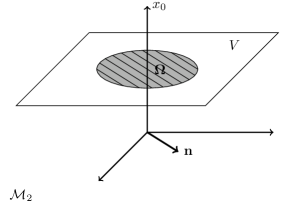
Figure 1: The embedding of the Bloch ball into ${\cal M}_{2}$ and its foliation by a flat convex roof.

Let us now consider the case where $\operatorname{Ker}Q$ does not contain a vector ${\bf n}$ with $n_{0}=0$. Then we have $\dim\operatorname{Ker}Q=1$ and this line intersects $V$ in one point which we call ${\bf n}$. Every other point $\bf m$ in $V$ can be connected to the point $\bf n$ by a line lying in $V$. Then $q^{1/2}$ is linear along the half-line $\mathbb{R}^{+}\ni s\mapsto s{\bf m}+(1-s){\bf n}$ since

$$q\left(s{\bf m}+(1-s){\bf n}\right) = (s{\bf m}+(1-s){\bf n})Q(s{\bf m}+(1-s){\bf n})$$ (14)

$$= s^{2}q({\bf m})$$

This concludes the proof of Theorem 3.

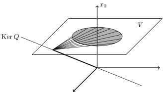
Figure 2: The foliation of the Bloch ball in the case $n_{0}\neq 0$.

Our proof of Theorem 4 presented in Hellmund and Uhlmann (2008a) used the Gorini-Sudarshan parametrization Gorini and Sudarshan (1976) of stochastic maps. Here we give a shorter and more elegant argument following Hildebrand (2006, 2007).

We will consider the flow of the signature of the quadratic form $q=q_{0}-w\eta$ as function of $w\in\mathbb{R}$. It is clear that for sufficiently large $w$ we have $\operatorname{sgn}q=\operatorname{sgn}(-\eta)=(+++-)$ whereas for large enough negative $w$ we have $\operatorname{sgn}q=\operatorname{sgn}(\eta)=(+---)$. A signature change can only occur at one of the real roots $w_{i}$ of $\det Q=\det(Q_{0}-w\eta)=0$. The “Minkowski metric” $\eta$ is regular and $\eta=\eta^{-1}$. Therefore the $w_{i}$ are the real eigenvalues of $\eta Q_{0}$ since $\det Q=(\det\eta)\det(\eta Q_{0}-wI)$.

Positivity of $\Phi$ implies $q^{\Phi}_{0}(\bf x)\geq 0$ for all $\bf x$ with $\bf x\cdot\bf x\geq 0$. This is just the assumption of Yakubovich’s S-lemma from the theory of quadratic forms (see Pólik and Terlaky (2007); Hildebrand (2006, 2007) which ensures the existence of a non-negative value $\hat{w}$ such that $q_{w}^{\Phi}$ is at least positive semidefinite, $q^{\Phi}_{\hat{w}}\geq 0$. Then it is clear that all four eigenvalues of $\eta Q_{0}$ are real and that $w_{1}\geq\hat{w}\geq w_{2}\geq w_{3}\geq w_{4}$: There must be at least one signature change above or at $\hat{w}$ and at least 3 signature changes below or at $\hat{w}$. More signature changes are impossible since we have at most four real roots. There is (up to degeneracies) only one possible pattern of signature changes and $q$ is positive and degenerate, $\operatorname{sgn}q=(+,..,0)$, precisely at $w=w_{1}$ and $w=w_{2}$. It is positive definite for $w_{1}>w>w_{2}$ if $w_{1}\neq w_{2}$. In the case $w_{1}\neq w_{2}$ let ${\bf n}_{1},{\bf n}_{2}$ be the corresponding vectors in $\operatorname{Ker}Q_{w_{i}}$. Then ${\bf n}_{1}Q_{0}{\bf n}_{1}=w_{1}{\bf n}_{1}^{2}$ and ${\bf n}_{2}Q_{0}{\bf n}_{2}=w_{2}{\bf n}_{2}^{2}$. Furthermore, no nonzero vector can be both in $\operatorname{Ker}Q_{w_{1}}$ and $\operatorname{Ker}Q_{w_{2}}$ since $\eta$ is non-degenerate. So, ${\bf n}_{1}Q_{0}{\bf n}_{1}>w_{2}{\bf n}_{1}^{2}$ and ${\bf n}_{2}Q_{0}{\bf n}_{2}>w_{1}{\bf n}_{2}^{2}$ (since $Q_{w_{1,2}}\geq 0$), providing $(w_{1}-w_{2}){\bf n}_{2}^{2}<0$ and $(w_{1}-w_{2}){\bf n}_{1}^{2}>0$. Therefore, $\operatorname{Ker}Q$ is time-like at $w_{1}$ and space-like at $w_{2}$.

In the degenerate case $w_{1}=w_{2}$, $\operatorname{Ker}Q$ is at least two-dimensional. In this case, let ${\bf n}_{1},{\bf n}_{2}$ be two orthogonal (in the Euclidean sense) vectors from $\operatorname{Ker}Q$. Then ${\bf n}_{1}$ and ${\bf n}_{2}$ can not both be time-like (since there is only one time-like direction).

This proofs the claim of Theorem 4, existence of a suitable $w_{0}$. It is given by $w_{2}$, the second largest eigenvalue of $\eta Q_{0}^{\Phi}$.

IV Explicit examples

Let us demonstrate our construction on some examples. From here on we will sometimes denote the coordinates $x_{1},x_{2},x_{3}$ of state space Eq. (III) as $x,y$ and $z$.

IV.1 Bistochastic maps or unital channels

Bistochastic maps preserve the center of the Bloch ball. We have $\vec{t}=0$ and the Bloch ball is pinched by ${\bf\Lambda}=\operatorname{diag}(\lambda_{1},\lambda_{2},\lambda_{3})$. This includes the depolarising channel $\rho\mapsto p\rho+(1-p)\frac{1}{2}I$ where ${\bf\Lambda}=\operatorname{diag}(p,p,p)$ and also the phase-damping channel where ${\bf\Lambda}=\operatorname{diag}(p,p,1)$. We get $w=\max(\lambda_{1}^{2},\lambda_{2}^{2},\lambda_{3}^{2})$ and

$$C_{\Phi}(\rho)=q^{1/2}_{\Phi}(\rho)=\sqrt{(1-w)x_{0}^{2}+\sum_{i=1}^{3}\left(w-\lambda_{i}^{2}\right)x_{i}^{2}}$$ (15)

which is flat in one direction since one of the terms in the sum vanishes.

Nevertheless, this case includes channels of all Kraus lengths between 1 and 4.

Since the roof is flat, the entanglement entropy is given by

$$E_{\Phi}(\rho)=\xi\left(\sqrt{(1-w)x_{0}^{2}+\sum_{i=1}^{3}\left(w-\lambda_{i}^{2}\right)x_{i}^{2}}\right).$$ (16)

The Holevo quantity $\chi^{*}_{\Phi}(\rho)$ (see Eq. 3) is a concave function. Since the channel is symmetric under all 3 reflections $x_{i}\mapsto-x_{i}$, it must take its maximum, the HSW capacity

$$\chi_{\Phi}=\max_{\rho}\chi^{*}_{\Phi}(\rho)$$ (17)

at the origin of the Bloch ball, $\rho=\frac{1}{2}I$. This reproduces the well-known Ohya et al. (1997) result

$$\chi_{\Phi}=S(\frac{1}{2}I)-\xi(\sqrt{1-w})=\log(2)-\eta(\frac{1+\sqrt{w}}{2})-\eta(\frac{1-\sqrt{w}}{2})$$ (18)

IV.2 Channels of Kraus length 2

A channel has Kraus length two if it can be represented as

$$\Phi(\rho)=A^{\dagger}\rho A+B^{\dagger}\rho B$$ (19)

The concurrence of such channels has already been studied in Uhlmann (2005) using a quite different approach. According to Ruskai et al. (2002), unitary transformations can bring such a channel to the form

$${\bf\Lambda} = \operatorname{diag}(\cos u,\cos v,\cos u\cos v)$$ (20)

$$\vec{t} = (0,0,\sin u\sin v)$$ (21)

which corresponds to $A=[\cos\frac{u}{2}\cos\frac{v}{2}]I+[\sin\frac{u}{2}\sin\frac{v}{2}]\sigma_{z},\;B=[\cos\frac{u}{2}\sin\frac{v}{2}]\sigma_{x}-i[\sin\frac{u}{2}\cos\frac{v}{2}]\sigma_{y}$ and we can assume $\cos u\geq\cos v$. Then we find for the concurrence $w=\cos^{2}u$ and

$$C_{\Phi}^{2}(\rho)=y^{2}(\cos^{2}(u)-\cos^{2}(v))+(z\cos u\sin v-\cos v\sin u)^{2}$$ (22)

which is positive semi-definite and independent of $x$, so we have again a flat roof. All channels which arise from a bipartite $2\times 2$ system with rank-2 input states via restriction of the partial trace to the support space of the input state are of length 2 and have therefore a flat roof, in accordance with Wootters’ celebrated result Hill and Wootters (1997); Wootters (1998).

IV.3 Axial symmetric channels

Every positive trace-preserving linear map commuting with rotations about the $x_{3}$-axis is (modulo unitary transformations) of the form

$$\Phi(\rho)=\begin{pmatrix}\alpha x_{00}+(1-\gamma)x_{11}&\beta x_{01}\\ \beta x_{10}&\gamma x_{11}+(1-\alpha)x_{00}\end{pmatrix}.$$ (23)

with real non-negative parameters $\alpha,\beta,\gamma$. The Bloch ball is pinched by ${\bf\Lambda}=\operatorname{diag}(\beta,\beta,\alpha+\gamma-1)$ and then shifted along the $x_{3}$-axis by $\vec{t}=(0,0,\alpha-\gamma)$.

This family includes many standard channels. Besides the

• phase-damping channel (length 2, unital) for $\alpha=\gamma=1$ and

• the depolarizing channel (length 4, unital) for $\alpha=\gamma,\;\beta=2\alpha-1$

which we already considered, we also find

• the amplitude-damping channel (length 2, non-unital) for $\gamma=1,\;\beta^{2}=\alpha$.

Positivity of $\Phi$ demands

$$0 \leq\;\alpha,\gamma \leq\;1,$$ (24)

$$\beta^{2} \leq\;\beta^{2}_{\text{max}} =\;1+2\alpha\gamma-\alpha-\gamma+2\sqrt{\alpha(1-\alpha)\gamma(1-\gamma)}.$$ (25)

The first inequality guarantees that north and south pole of the Bloch ball are not mapped to the outside, the the second one describes the limit when the ellipsoid touches the sphere at a circle.

Figure 3: A map which is at the boundary of the set of positive maps.

The stronger condition of complete positivity of $\Phi$ evaluates to

$$\beta^{2}\leq\alpha\gamma$$ (26)

For the concurrence we have found the explicit expression

$$C^{2}_{\Phi}(X)=4(\det\Phi(X)-w\det(X))$$ (27)

with

$$w = \max(\beta^{2},\beta^{2}_{c})$$ (28)

$$\text{where}\qquad\beta_{c}^{2} = 1+2\alpha\gamma-\alpha-\gamma-2\sqrt{\alpha(1-\alpha)\gamma(1-\gamma)}.$$ (29)

In the case $\beta\geq\beta_{c}$ we have a flat roof whose leaves are in planes perpendicular to the $z$-axis.

Figure 4: Leaves of the concurrence at $\beta>\beta_{c}$.

In the other case we have a one-dimensional $\operatorname{Ker}Q$ generated by ${\bf n}=(1,0,0,z_{0})$ with $z_{0}=\frac{\sqrt{\gamma(1-\gamma)}+\sqrt{\alpha(1-\alpha)}}{\sqrt{\gamma(1-\gamma)}-\sqrt{\alpha(1-\alpha)}}$. The roof is not flat. The leaves are straight lines meeting at the point $z_{0}$ on the $z$-axis outside the Bloch ball:

Figure 5: Leaves of the concurrence at $\beta<\beta_{c}$.

At the bifurcation point $\beta=\beta_{c}$ the concurrence is linear everywhere on the Bloch ball (and therefore every decomposition is optimal):

$$C_{\beta=\beta_{c}}(\rho)=\left(\sqrt{\alpha(1-\alpha)}-\sqrt{\gamma(1-\gamma)}\right)z+\sqrt{\alpha(1-\alpha)}+\sqrt{\gamma(1-\gamma)}$$ (30)

The special case of the amplitude-damping channel $\alpha=\beta^{2},\gamma=1$ and therefore $\beta=\beta_{c}=\beta_{max}$ belongs to this degenerate situation with

$$C_{AD}(\rho)=(1+z)\sqrt{\alpha(1-\alpha)}$$ (31)

Since this channel has length 2, this result is also a special case of eq. (22) for $u=-v$ with $\alpha=\cos^{2}u$. The concave Holevo quantity must take its maximum for states on the z-axis where we get

$$\chi^{*}_{AD}(z)=\eta\left(\frac{1+z}{2}\alpha\right)+\eta\left(1-\frac{1+z}{2}\alpha\right)-{\xi}\left((1+z)\sqrt{\alpha(1-\alpha)}\right)$$ (32)

The equation $\frac{\partial\chi^{*}}{\partial z}=0$ can be solved only numerically. The resulting capacity is plotted in Fig. 6.

Figure 6: HSW capacity for the amplitude-damping channel as function of the channel parameter $\alpha$.

Similar results can be found in Dorlas and Morgan (2008).

Let us finally mention that we have no explanation for the striking similarity between eqs. (25) and (29). They differ only by the sign of the square root. So, $\beta^{2}_{max}$ derived from Fig. 3 and this $\beta^{2}_{c}$ of the roof bifurcation are roots of the same quadratic equation.

IV.4 The $2\times n$ bipartite quantum system

Here we consider $2\times n$ systems $\mathcal{H}=\mathcal{H}^{A}\otimes\mathcal{H}^{B}$, $\dim\mathcal{H}^{A}=2$. Let $\mathcal{H}_{2}$ be any 2-dimensional subspace of $\mathcal{H}$ and $V$ a unitary mapping of $\mathcal{H}^{A}$ onto $\mathcal{H}_{2}$. Then

$$\rho\mapsto\Phi(\rho)=V(\operatorname{Tr}_{B}\rho)V^{{\dagger}}$$ (33)

is a 1-qubit channel for all density operators $\rho$ supported by $\mathcal{H}_{2}$. The eigenvalues of $\Phi(\rho)$ and of $\rho^{A}=\operatorname{Tr}_{B}\rho$ are the same. Hence, by Eq. (11) and by Theorem 4, we are allowed to write

$$C(\rho)^{2}=4(\det\rho^{A}-w\det\rho)$$ (34)

for all density operators $\rho$ with support in $\mathcal{H}_{2}$ and with a unique $w=w(\mathcal{H}_{2})$. Notice that this representation does not depend on the choice of the unitary $V$ in Eq. (33). However, $w$ depends on the 2-dimensional subspace $\mathcal{H}_{2}$.

As an illustrating example we choose $n=4$ and consider $\mathcal{H}^{B}$ as a 2-qubit system. Then $\mathcal{H}$ becomes a 3-qubit system, $\mathcal{H}=\mathcal{H}^{a}\otimes\mathcal{H}^{b}\otimes\mathcal{H}^{c}$, and the partial trace $\operatorname{Tr}_{B}$ from Eq. (33) is identified with $\operatorname{Tr}_{bc}$. An interesting subspace is generated by the W and GHS state vectors given by $|W\rangle=3^{-1/3}(|001\rangle+|010\rangle+|100\rangle)$ and $|GHS\rangle=2^{-1/2}(|000\rangle+|111\rangle)$. Defining the unitary $V$ in Eq. (33) by $V|0\rangle=|GHZ\rangle$ and $V|1\rangle=|W\rangle$, $\Phi$ can be computed to be the 1-qubit map

$$\begin{pmatrix}x_{00}&x_{01}\\ x_{10}&x_{11}\end{pmatrix}\,\mapsto\,\begin{pmatrix}\frac{2}{3}x_{00}+\frac{1}{2}x_{11}&\frac{1}{\sqrt{6}}x_{01}\\ \frac{1}{\sqrt{6}}x_{10}&\frac{1}{3}x_{00}+\frac{1}{2}x_{11}\end{pmatrix}$$ (35)

This an axial symmetric channel and we can read off $w=1/6$, therefore,

$$C^{2}(\rho)=\frac{8}{9}x_{00}^{2}+x_{11}^{2}+\frac{4}{3}x_{00}x_{11}$$ (36)

For $\rho$ supported in our subspace this is equivalent to

$$C(\rho)^{2}=\frac{8}{9}\langle GHZ|\rho|GHZ\rangle^{2}+\langle W|\rho|W\rangle^{2}+\frac{4}{3}\langle GHZ|\rho|GHZ\rangle\,\langle W|\rho|W\rangle$$ (37)

After this quite explicit example we return to the more general case of Eq. (34). We rewrite the $2\times 2$ determinants in Eq. (34) by the help of the characteristic equation in terms of traces:

$$C(\rho)^{2}=2[(\operatorname{Tr}\rho^{A})^{2}-\operatorname{Tr}((\rho^{A})^{2})]-2w[(\operatorname{Tr}\rho)^{2}-\operatorname{Tr}(\rho^{2})]$$ (38)

Polarization of this quadratic form provides (compare Eq. (11)) the bilinear form

$$q_{w}(\rho_{1},\rho_{2})=2(1-w)(\operatorname{Tr}\rho_{1})(\operatorname{Tr}\rho_{2})+2\left[w(\operatorname{Tr}\rho_{1}\rho_{2})-(\operatorname{Tr}\rho_{1}^{A}\rho_{2}^{A})\right]$$ (39)

defined for all pairs of Hermitian operators on $\mathcal{H}$. If $\rho_{1}$ and $\rho_{2}$ are supported by the same 2-dimensional subspace $\mathcal{H}_{2}$, and if $w$ is correctly chosen, then $q_{w}$ is positive semi-definite and degenerate on that subspace. Hence, if $C(\rho_{1})=0$, then also $q_{w}(\rho_{1},\rho_{2})=0$ for all $\rho_{2}$ supported by $\mathcal{H}_{2}$. In particular, if $\rho_{1}=\pi_{1}$ is a separable pure state and $\rho_{2}$ a state, we get

$$1-\operatorname{Tr}\pi_{1}^{A}\rho_{2}^{A}=w(1-\operatorname{Tr}\pi_{1}\rho_{2})$$ (40)

It holds $\pi_{1}=\pi_{1}^{A}\otimes\pi_{1}^{B}$, as $\pi_{1}$ is assumed separable.
If there is a second pure separable state, say $\pi_{2}$, supported by $\mathcal{H}_{2}$, one gets

$$1-\operatorname{Tr}\pi_{1}^{A}\pi_{2}^{A}=w(1-(\operatorname{Tr}\pi_{1}^{A}\pi_{2}^{A})\,(\operatorname{Tr}\pi_{1}^{B}\pi_{2}^{B}))$$ (41)

Thus, in this particular case, the number $w$ is determined by the transition probabilities $\operatorname{Tr}\pi_{1}^{A,B}\pi_{2}^{A,B}=|\langle\psi^{A,B}_{1}|\psi_{2}^{A,B}\rangle|^{2}$ between the marginal states of $\pi_{1}$ and $\pi_{2}$. One observes that $w$ can vary between 0 and 1 already for subspaces generated by two separable vectors. This is a nice illustration of Theorem 3: The operator $\pi_{2}-\pi_{1}$ belongs to ${\rm Ker}\,Q$, and the concurrence remains constant along the intersection of the Bloch ball carried by $\mathcal{H}_{2}$ with every real line of the form $\rho+t(\pi_{2}-\pi_{1})$.

V Entanglement entropy for axial symmetric stochastic 1-qubit maps

In this chapter we study the entanglement entropy $E_{\Phi}$ defined in Eq. (1) for the axially symmetric map Eq. (23) in more detail, using Theorem 2 and numerical methods.

Our aim is an understanding of the structure of the foliation of the Bloch ball provided by the convex roof construction. This foliation encodes the optimal decompositions Eq. (2) for all states. The foliation changes with the channel parameters. In most of the $(\alpha,\beta,\gamma)$ parameter space all states have an optimal decomposition into two pure states. In a small region of the parameter space we find optimal decompositions of length 3. We characterize the bifurcation structure of this “phase transition” and its position in parameter space.

There exist quite a lot numerical and analytical work about the HSW capacity of 1-qubit channels, e.g., Cortese (2002); Berry (2005); Li-Zhen and Mao-Fa (2007) where the optimal decomposition of the optimal state is considered. In contrast, we consider the optimal decomposition of all states.

V.1 Some degenerate channels

$\alpha=\gamma$

In this case the channel is unital and has therefore a flat convex roof for the concurrence. We have $\beta_{\text{max}}=1$ and $\beta_{c}^{2}=(2\alpha-1)^{2}$, so we find $w=\max((2\alpha-1)^{2},\,\beta^{2})$. The concurrence $C$, and hence $E_{\Phi}$ too, are constant either (in case of $(2\alpha-1)^{2}>\beta^{2}$) on concentric cylinders around the $z$-axis $E_{\Phi}=E_{\Phi}(x^{2}+y^{2})$ or on planes perpendicular to the $z$-axis $E_{\Phi}=E_{\Phi}(z)$.

$\alpha+\gamma=1$

In this case the range of the channel is degenerate, being a 2-dimensional ellipse orthogonal to the $z$-axis. Furthermore, $\beta_{c}=0$ and therefore $w=\beta^{2}$. We get again a flat roof. $C_{\Phi}(z)$ and hence $E_{\Phi}$, too, are constant on planes perpendicular to the $z$-axis.

V.2 The general case $(\alpha-\gamma)(\alpha+\gamma-1)\neq 0$

We did extensive numerical studies of the global minimization problem of the entanglement entropy Eq. (1), guided by and compared to analytic studies of special cases. The following overall picture emerged: There are 3 different phases. For fixed values of $\alpha$ and $\gamma$, we have at large values of $\beta$ a phase (phase I) where the entanglement depends only on $z$. By decreasing $\beta$, we reach phase II where a cone with apex at the north pole appears. States in the cone have optimal decompositions of length 3. The opening angle of the cone decreases and for small enough $\beta$ we reach phase III, where again all optimal decompositions have length 2.

Figure 7: Leaves of the foliation of the entanglement entropy. The $z$ axis points upwards.

Of course we have a flat entanglement roof as long as we have a flat concurrence roof (phase Ia). But the flat phase for the entanglement extends to even lower values of $\beta$, where the concurrence is not longer flat (phase Ib)!

For phase III let us remark that the leaves form cones with their apex on the $z$-axis outside the Bloch ball. But different to the Phase II of the concurrence (compare Fig. 5) they do not intersect at the same point on the $z$-axis.

The above picture and the equations for $\beta_{1}$ and $\beta_{2}$ below are valid in the case

$$(\alpha-\gamma)(\alpha+\gamma-1)>0.$$ (42)

For the opposite case, turn the pictures upside down ($z\rightarrow-z$) and exchange $\alpha\leftrightarrow\gamma$ in the equations below for $\beta_{1}$ and $\beta_{2}$.

The bifurcation points $\beta_{1}$ and $\beta_{2}$ between the 3 phases can be calculated analytically. Let $s(\cos(\phi))$ denote the entropy $S(\Phi(\pi))$ for the pure state $\pi=(\sin(\phi),0,\cos(\phi))$. Then the bifurcation point $\beta_{1}$ can be found by comparing the competing decompositions $E_{1}=\frac{1}{3}s(1)+\frac{2}{3}s(\cos(\phi))$ with $E_{2}=s(\frac{1}{3}+\frac{2}{3}\cos(\phi))$. We expand $E_{1}(\phi)-E_{2}(\phi)=g(\alpha,\beta,\gamma)\phi^{2}+O(\phi^{3})$ and get $\beta_{1}$ as the root of $g(\alpha,\beta,\gamma)=0$.

Using the abbreviations $x=2\alpha-1,y=2\gamma-1$ we find

$$\begin{split}\beta_{1}^{2}=&\frac{x}{2(x+(x^{2}-1)\operatorname{arctanh}(x)}\left(x^{2}+xy+(x^{2}-1)y\operatorname{arctanh}(x)-\right.\\ &\left.\sqrt{(1-x^{2})\operatorname{arctanh}(x)(x^{3}-xy^{2}-(x^{2}-1)y^{2}\operatorname{arctanh}(x))}\right)\end{split}$$ (43)

Analogously, we obtain $\beta_{2}$ by comparing the decompositions $E_{1}=\frac{1+\cos(\phi)}{2}s(1)+\frac{1-\cos(\phi)}{2}s(-1)$ and $E_{2}=s(\cos(\phi))$ around $\phi=\pi$:

$$\beta_{2}^{2}=y\,\frac{(1+x)\log(1-y)+(1-x)\log(1+y)-(1+x)\log(1+x)-(1-x)\log(1-x)}{2(\log(1-y)-\log(1+y))}$$ (44)

V.3 Phase diagram

The following figure shows the phases in the $\beta,\gamma$-plane for $\alpha=0.8$. The upper boundary is given by the positivity condition, Eq. (25). The boundary between phases Ia (entanglement and concurrence have flat roofs) and Ib (only entanglement has flat roof) is given by Eq. (29). Phase II is bounded by Eqs. (43) and (44).

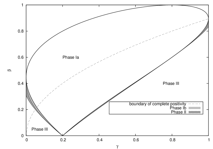
Figure 8: Phase diagram in the $(\gamma,\beta)$-plane for $\alpha=0.8$.

The phase II region where length 3 optimal decompositions exist as well as the phase Ib are quite small but they exist everywhere outside the degenerate points where either $\alpha+\gamma=1$ or $\alpha=\gamma$.

V.4 One-shot (HSW) capacity

The Holevo quantity will take its maximum for a state on the $z$-axis. Its numerical calculation is highly simplified by taking the foliation structure into account. We show in Figure 9 the $\beta$ dependence of this maximum, i.e., the HSW capacity, for fixed values of $\alpha$ and $\gamma$. The maps are positive for $\beta\leq\beta_{max}$, completely positive for $\beta\leq\beta_{cp}$. The values $\beta_{1}$ and $\beta_{2}$ indicated in the figure separate the phases I, II and III. In phase III the capacity is independent of $\beta$.

Figure 9: The HSW capacity as function of the channel parameter $\beta$ at $\alpha=0.8,\;\gamma=0.4$. The inset shows the small region where the transition between phases I, II and III takes place.

VI Concurrence for channels with higher input or output rank

Our method provides a complete solution for the concurrence of trace-preserving positive maps of input and output rank 2. How could one possibly overcome the input rank two (or 1-qubit map) restriction? The following problem may be of interest: Assume $\sum p_{j}\pi_{j}$ is an optimal decomposition for the concurrence of a $2\times n$ system. Every pair $\pi_{j}$, $\pi_{k}$ of different pure states is supported by a 2-dimensional Hilbert space $\mathcal{H}_{jk}$. Hence there is a number $w_{jk}=w(\mathcal{H}_{jk})$ defining the concurrence for density operators supported by $\mathcal{H}_{jk}$ according to Eq. (34). Which restrictions on the set of all $w_{jk}$ arise from the optimality of the decomposition?

Another issue is the generalization to higher output ranks. Rungta et al Rungta et al. (2001) proposed to replace the determinant $\det\rho$ by the second elementary symmetric function of the eigenvalues, $C_{\Phi}(\pi)=2\sqrt{e_{2}(\Phi(\pi))}$. While the square root of $e_{2}$ is concave, one might find a value for $w$ making the expression

$$2\sqrt{e_{2}(\Phi(\rho))-w\,e_{2}(\rho)}$$ (45)

a convex extension of $2e_{2}(\Phi(\pi))^{1/2}$, $\pi$ pure. In these cases, the expression Eq. (45) is a lower bound for the $\Phi$-concurrence. An example is the diagonal map $D_{m}$ in any dimension $m$ which cancels the off-diagonal elements. Denoting the matrix elements of $\rho$ by $x_{jk}$, this recipe results in

$$C_{D}(\rho)\geq 2(\sum_{j<k}|x_{jk}|^{2})^{1/2}$$ (46)

Another example is the following family of indecomposable Choi maps of a $3\times 3$ system:

$$\rho\;\mapsto\;\Phi[\mu](\rho)\;=\;\frac{1}{1+\mu}\begin{pmatrix}x_{00}+\mu x_{22}&-x_{01}&-x_{02}\\ -x_{10}&x_{11}+\mu x_{00}&-x_{12}\\ -x_{20}&-x_{21}&x_{22}+\mu x_{11}\end{pmatrix}.$$ (47)

$\Phi[\mu]$ is trace-preserving, positive and indecomposable for $\mu\geq 1$. The map $\Phi[1]$ is extremal in the set of positive maps. Here our recipe provides the bound

$$C_{\Phi}(\rho)^{2}\geq\frac{4\mu}{(1+\mu)^{2}}\left[(x_{00}+x_{11}+x_{22})^{2}+(\mu-1)\left(|x_{01}|^{2}+|x_{02}|^{2}+|x_{12}|^{2}\right)\right],$$ (48)

a positive semi-definite quadratic form in the matrix entries. In the special case $\mu=1$ our recipe provides an exact though highly degenerate answer: $\Phi[1]$ maps all pure states of the $3\times 3$ system to mixed states with the same $\Phi$-concurrence and therefore the $\Phi$-concurrence is constant everywhere, $C_{\Phi}(\rho)=1.$

VII Conclusions

We have explained a way to get concurrences of stochastic 1-qubit maps and of rank two states in $2\times n$ quantum systems. The methods is attractive by its simplicity, providing a large area of applications. The new methods is different from that of Wootters Wootters (1998) and of Uhlmann (2000) which is based on conjugations.

The advantage of the new methods is its applicability to roofs which are not flat. Only a small subset of the stochastic 1-qubit maps actually has a $\Phi$-concurrence which is a flat roof. For a general 1-qubit map the concurrence is real linear on each member of a unique bundle of straight lines crossing the Bloch ball. The bundle consists either of parallel lines or the lines meet at a pure state, or they meet at a point outside the Bloch ball. Furthermore, $C_{\Phi}$ turns out to be the restriction of a Hilbert semi-norm to the state space.

For the special case of an axial symmetric 1-qubit channel we presented a throughout study of the $\Phi$-entanglement. Here the structure of the optimal decomposition of states can be quite different depending on the channel parameters. There is a phase where all optimal decompositions have length 2 and are flat, a phase where states with optimal decompositions of length 3 exist, forming a cone in the foliation of the Bloch ball, and a phase where all optimal decompositions are of length 2 but not flat. We found explicit formulas for the bifurcation points which separate the phases. Interestingly, there exists a region in the space of 1-qubit maps where the $\Phi$-entanglement is flat despite the fact that the $\Phi$-concurrence is not flat.

Our method of finding optimal decompositions for the concurrence works perfectly for rank two density operators only. For higher rank states it provides lower bounds. It is a challenge to find an algorithm, if existing, which combines the merits of this approach and the conjugation based one.

Appendix A

The function defined in Eq. (6)

$$\xi(x)=H\left(\frac{1-y}{2},\frac{1+y}{2}\right),\quad 1=x^{2}+y^{2}$$ (49)

is defined on $-1\leq x\leq 1$ and does not depend on the sign of $x$. It is strictly convex since

$$\xi^{\prime\prime}(x) = \frac{1}{2y^{3}}\ln\frac{1+y}{1-y}-\frac{1}{y^{2}}$$ (50)

$$= \frac{1}{y^{2}}\left(\frac{y^{3}}{3}+\frac{y^{5}}{5}+\frac{y^{7}}{7}+\cdots\right)\;>\;0$$ (51)

Therefore, $\xi$ is the supremum of a family of functions $ax+b$. Inserting a convex function $C(\rho)$ with values $-1\leq C\leq 1$ represents $\xi(C)$ by a supremum of convex functions $aC+b$. This proves the convexity of $\xi(C(\rho))$ as a function of $\rho$.

References

- Nielsen and Chuang (2000) M. A. Nielsen and I. L. Chuang, Quantum Computation and Quantum Information (Cambridge University Press, 2000).
- Petz (2008) D. Petz, Quantum Information Theory and Quantum Statistics (Springer, 2008).
- (3) R. Horodecki, P. Horodecki, M. Horodecki, and K. Horodecki, Quantum entanglement, Rev. Mod. Phys., to appear, eprint quant-ph/0702225.
- Bengtsson and Życzkowski (2006) I. Bengtsson and K. Życzkowski, Geometry of Quantum States (Cambridge University Press, 2006).
- Bennett et al. (1996) C. H. Bennett, D. P. DiVincenzo, J. A. Smolin, and W. K. Wootters, Physical Review A 54, 3824 (1996), eprint quant-ph/9604024.
- Schumacher and Westmoreland (1997) B. Schumacher and M. D. Westmoreland, Phys. Rev. A 56, 131 (1997).
- Holevo (1998) A. S. Holevo, IEEE Transactions on Information Theory 44, 269 (1998), quant-ph/9611023.
- Terhal and Vollbrecht (2000) B. M. Terhal and K. G. H. Vollbrecht, Phys. Rev. Lett. 85, 2625 (2000).
- Vollbrecht and Werner (2001) K. G. H. Vollbrecht and R. F. Werner, Phys. Rev. A 64, 062307 (2001), eprint quant-ph/0010095.
- Benatti et al. (1996) F. Benatti, H. Narnhofer, and A. Uhlmann, Rep. Math. Phys 38, 123 (1996).
- Hill and Wootters (1997) S. Hill and W. K. Wootters, Phys. Rev. Lett. 78, 5022 (1997), eprint quant-ph/9703041.
- Wootters (1998) W. K. Wootters, Phys. Rev. Lett. 80, 2245 (1998), eprint quant-ph/9709029.
- Wootters (2001) W. K. Wootters, Quantum Information and Computation 1, 27 (2001).
- Łoziński et al. (2003) A. Łoziński, A. Buchleitner, K. Życzkowski, and T. Wellens, Europhysics Letters 62, 168 (2003), eprint quant-ph/0302144.
- Chen et al. (2005) K. Chen, S. Albeverio, and S.-M. Fei, Physical Review Letters 95, 040504 (2005), quant/ph-0506136.
- Ou et al. (2007) Y.-C. Ou, H. Fan, and S.-M. Fei (2007), arXiv:0711.2865.
- Hellmund and Uhlmann (2008a) M. Hellmund and A. Uhlmann, Concurrence of stochastic 1-qubit maps (2008a), arXiv:0802.209.
- Hildebrand (2007) R. Hildebrand, J. Math. Phys. 48, 102108 (2007).
- Hildebrand (2006) R. Hildebrand, Concurrence of Lorentz-positive maps (2006), eprint quant-ph/0612064.
- Horodecki et al. (1996) M. Horodecki, P. Horodecki, and R. Horodecki, Phys. Lett. A 223, 1 (1996).
- Uhlmann (1998) A. Uhlmann, Open Sys. Information Dyn. 5, 209 (1998), eprint quant-ph/9701014.
- Rockafellar (1970) R. T. Rockafellar, Convex Analysis (Princeton University Press, 1970).
- Fuchs and van de Graaf (1999) C. A. Fuchs and J. van de Graaf, IEEE Transactions on Information Theory 45, 1216 (1999), eprint quant-ph/9712042.
- Hellmund and Uhlmann (2008b) M. Hellmund and A. Uhlmann, An entropy inequality (2008b), arXiv:0812.0906, Quant. Inf. Comp., to appear.
- King and Ruskai (2001) C. King and M. B. Ruskai, IEEE Transactions on Information Theory 47, 192 (2001), eprint quant-ph/9911079.
- Gorini and Sudarshan (1976) V. Gorini and E. C. G. Sudarshan, Commun. Math. Phys. 46, 43 (1976).
- Pólik and Terlaky (2007) I. Pólik and T. Terlaky, SIAM Review 49, 371 (2007).
- Ohya et al. (1997) M. Ohya, D. Petz, and N. Watanabe, Prob. Math. Stat. 17, 179 (1997).
- Uhlmann (2005) A. Uhlmann, Open Sys. Information Dyn. 12, 1 (2005), eprint quant-ph/0605103.
- Ruskai et al. (2002) M. B. Ruskai, S. Szarek, and E. Werner, Lin. Alg. and its Appl. 347, 159 (2002).
- Dorlas and Morgan (2008) T. C. Dorlas and C. Morgan, International Journal of Quantum Information 6, 745 (2008).
- Cortese (2002) J. Cortese, Relative entropy and single qubit Holevo-Schumacher-Westmoreland channel capacity (2002), eprint quant-ph/0207128.
- Berry (2005) D. W. Berry, Phys. Rev. A 71, 032334 (2005).
- Li-Zhen and Mao-Fa (2007) H. Li-Zhen and F. Mao-Fa, Chinese Physics 16, 1843 (2007).
- Rungta et al. (2001) P. Rungta, V. Bužek, C. M. Caves, M. Hillery, and G. J. Milburn, Phys. Rev. A 64, 042315 (2001), eprint quant-ph/0102040.
- Uhlmann (2000) A. Uhlmann, Physical Review A 62, 032307 (2000), eprint quant-ph/9909060.