Diffusion of single ellipsoids under quasi-2D confinements

Abstract

We report video-microscopy measurements of the translational and rotational Brownian motions of isolated ellipsoidal particles in quasi-two-dimensional sample cells of increasing thickness. The long-time diffusion coefficients were measured along the long ($D_{a}$) and short ($D_{b}$) ellipsoid axes, respectively, and the ratio, $D_{a}/D_{b}$, was determined as a function of wall confinement and particle aspect ratio. In three-dimensions this ratio ($D_{a}/D_{b}$) cannot be larger than two, but wall confinement was found to substantially alter diffusion anisotropy and substantially slow particle diffusion along the short axis.

I Introduction

In many biological and industrial processes, diffusing particles are non-spherical and move in confined geometries. Examples of particles in this scenario include proteins diffusing in membranes Saffman and Delbruck (1975) and very fine grains migrating through pores in porous media. To date, quantitative measurements of anisotropic particle diffusion in confined geometries have been limited. However, new particle fabrication and imaging technologies combined with new image analysis tools now make the direct measurement of the diffusion of anisotropic particles readily possible. Thus, in this contribution we investigate the anisotropic diffusion of isolated ellipsoidal particles confined between two parallel plates.

The Brownian diffusion coefficient $D$ of an isolated spherical particle is well understood. It is inversely proportional to the drag (or friction) coefficient $\gamma$ via the Einstein relation,

$$D=k_{B}T/\gamma$$ (1)

where $k_{B}$ is the Boltzmann constant and $T$ is the temperature. For a prolate spheroid with long axis of length $2a$ and two short axes of length $2b$, translational diffusion is anisotropic and is described by diffusion coefficients $D_{a}=k_{B}T/\gamma_{a}$ along the long axis, and $D_{b}=k_{B}T/\gamma_{b}$ along the short axes. The rotational diffusion coefficient of the prolate spheroid about its short axes is $D_{\theta}=k_{B}T/\gamma_{\theta}$. Generally, the drag coefficients $\gamma_{a}$, $\gamma_{b}$ and $\gamma_{\theta}$ depend on the shape and size of the ellipsoid. Brownian motion of anisotropic particles was first seriously considered by F. Perrin Perrin (1934, 1936) who computed these drag coefficients analytically for a spheroid diffusing in three dimensions (3D). Interestingly, the ratio $D_{a}/D_{b}$ varies from one to two in 3D, as the spheroid aspect ratio $\phi=a/b$ varies from one to infinity.

The problem of diffusion in confined geometries, such as quasi-2D media, is different from the 3D case as a result of a complex interplay between hydrodynamic drag, the boundaries of the medium, and the particle geometry. Surfaces near a moving particle modify fluid flow fields, often increasing particle hydrodynamic drag. A full theoretical formulation of wall hydrodynamic effects has been developed for one sphere (or ellipsoid) coupled to one wall Happel and Brenner (1991). However, for more complicated situations, such as a sphere or an ellipsoid confined by two parallel walls, the only available analytical solutions are for weak confinement in a few special symmetric configurations Happel and Brenner (1991). Recent numerical calculations Bhattacharya et al. (2005), on the other hand, have been developed to derive the hydrodynamic drag of a single sphere and a linear chain of spheres confined more strongly in quasi-2D.

On the experimental side, the hydrodynamic drag of single spheres in weak confinement have been measured Lin et al. (2000); Dufresne et al. (2001), and video microscopy has been applied recently to measure anisotropic particle diffusion, including ellipsoids in quasi-2D Han et al. (2006) and 3D Mukhija and Solomon (2007), colloidal clusters near one wall Kim et al. (2008), and carbon nanotubes in weak confinement Bhaduri et al. (2008). In the present contribution we report measurements of hydrodynamic drag on ellipsoids in quasi-2D, confined between two parallel walls. We explore the strong confinement regime where drag coefficients are not readily available from theory and simulation, and we report on a light interference method to accurately measure the confinement. We find that the diffusion anisotropy is made stronger and the diffusion along ellipsoid short axes is dramatically slowed due to wall confinement. The experiment and analyses are similar to a previous paper Han et al. (2006). However the scope of the present work is different, focusing instead on how confinement affects diffusion, rather than on the detailed time-dependent Brownian dynamics of a single ellipsoid with the greatest diffusion anisotropy.

II Theory background

When a spheroid with semi-axes ($a$, $b$, $b$) moves along one of its principle axes with velocity $v$, through an unbounded quiescent fluid with viscosity $\eta$ at low Reynolds number, then the translational and rotational (about short axis) drag coefficients affecting the spheroid are

$$\gamma=6\pi\eta bG,$$ (2a)

$$\gamma_{\theta}=6\eta VG_{\theta}.$$ (2b)

$V$ is the volume of the spheroid and $G$ is the geometric factor that renders the ellipsoid different relative to the case of a sphere. The geometric factors for prolate spheroids diffusing in 3D are analytically given by Perrin’s equations Happel and Brenner (1991):

$$G_{a}=\frac{8}{3}\frac{1}{\left[\frac{2\phi}{1-\phi^{2}}+\frac{2\phi^{2}-1}{(\phi^{2}-1)^{3/2}}\ln(\frac{\phi+\sqrt{\phi^{2}-1}}{\phi-\sqrt{\phi^{2}-1}})\right]},\\$$ (3a)

$$G_{b}=\frac{8}{3}\frac{1}{\left[\frac{\phi}{\phi^{2}-1}+\frac{2\phi^{2}-3}{(\phi^{2}-1)^{3/2}}\ln(\phi+\sqrt{\phi^{2}-1})\right]},\\$$ (3b)

and Koenig (1975); Perrin (1934)

$$G_{\theta}=\frac{2}{3}\frac{\phi^{4}-1}{\phi\left[\frac{2\phi^{2}-1}{\sqrt{\phi^{2}-1}}\ln(\phi+\sqrt{\phi^{2}-1})-\phi\right]}.\\$$ (3c)

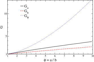
Figure 1: The geometric factors $G$ in Eq. (3) as a function of aspect ratio $\phi$.

Here $\phi=a/b$ is the aspect ratio. When $\phi=1$, then $G=G_{\theta}=1$, and Eq. (2) reduces to the translational and rotational Stokes laws for a sphere. Note also that Eqs. (2) and (3) are obtained using stick boundary conditions, valid when the particle is much larger than fluid molecules Hu and Zwanzig (1974); Bauer et al. (1974). In Fig. 1, Eq. (3) is plotted out as a function of $\phi$ for $\phi$ less than 10. When the aspect ratio $\phi\gg 1$, Eqs. (1), (2) and (3) yield

$$D_{a}=\frac{k_{B}T\ln\phi}{2\pi\eta a},\qquad D_{b}=\frac{k_{B}T\ln\phi}{4\pi\eta a}.$$ (4)

The ratio between these diffusion coefficients along long and short axes, i.e. $D_{a}/D_{b}=G_{b}/G_{a}$, increases monotonically from one to two as $\phi$ increases from one to infinity (in 3D). In quasi-2D, however, $D_{a}/D_{b}$ can be larger than two.

III Experiment

The diffusion of micrometer size PMMA (polymethyl methacrylate) and PS (polystyrene) ellipsoids was measured in water confined between two glass walls. Both PS and PMMA ellipsoids are synthesized by the method described in Ref. Ho et al. (1993). Briefly, we placed 0.5% (by weight) PS spheres into a 12% (by weight) aqueous PVA (polyvinyl alcohol) solution residing in a Petri dish. After water evaporation, the PVA film was stretched at 130^∘C. The PS (or PMMA) spheres embedded in the film are readily stretched because their glass transition temperatures are below 130^∘C. After cooling to room temperature, the PVA was dissolved and ellipsoids obtained. Note, the initial PMMA or PS spheres must not be cross-linked, otherwise they cannot be stretched. We measured the size of ellipsoids by SEM and by optical microscopy.

The ellipsoid solutions were cleaned and stabilized with 7 mM SDS (sodium dodecyl sulfate). The ellipsoids were not expected to have strong interactions with the glass surfaces, because the solution ionic strength was more than 0.1 mM and the Debye screening length for the particles was correspondingly less than 30 nm. However, it is difficult to estimate the ionic strength accurately in a thin cell because the glass surfaces can release Na⁺ ions Crocker (1996). Nevertheless, we found that the addition of 2 mM salt to the solution did not induce a detectable change in particle diffusion coefficients. This observation suggests that the double layers are not significantly affecting particle diffusion.

Glass surfaces of the sample cell were rigorously cleaned in a 1:4 mixture of hydrogen peroxide and sulfuric acid by sonication. Then the glass was thoroughly rinsed in deionized water and quickly dried with an air blow gun. Typically 0.3 $\mathrm{\mu L}$ solution spread over the entire $1.8\times 1.8~{}\textrm{mm}^{2}$ coverslip area, and ellipsoids did not stick to the surfaces. Because the gravitational height, $k_{B}T/mg$, is much larger than the cell thickness, $H$, the ellipsoids were readily suspended around mid-plane between the two walls. Finally, the cell was sealed with UV cured adhesive (Norland 63).

We measure the wall separation by light interference. When the cell thickness is below a few micrometers, then the interference colors produced by reflections from the two inner surfaces of the sample walls in white light illumination can be observed by eye or in the reflection mode of microscope, see Fig. 2A,B. When the wall separation $H=0$, the effective light path difference is $\Delta l=\lambda/2$ due to the $\pi$ phase shift of reflection at the lower surface. Thus all wavelength components of the white light yield a dark black color in interference at $H=0$. When $H>0$, the reflection light in the normal direction is a mixture of light with various wavelengths, and different wavelengths contribute with different weights to the observed color. White light interference from a wedge, for example, will be bands of colors as in the Michel-Levy Chart Hartshorne and Stuart (1970). By comparing the observed color with the Michel-Levy Chart, we can effectively read out the corresponding $\Delta l$ and obtain $H=\Delta l/(2n_{w})$, where $n_{w}$ is the refractive index of water. In the Michel-Levy Chart, the color starts from black at $\Delta l=0$ and changes from red to blue periodically with period $\Delta l=625$ nm. To avoid misreading the color by one or more periods, we either made a reference wedge or we put dilute spacer spheres with known diameter between the glass slides to establish a reference thickness. Also, color bands may shift slightly because the illumination light is not an ideal white light source. This error however, should be less than $625/4~{}\textrm{nm}$, so that the error of $H$ is less than $\delta H~{}(625$ nm$/4)/(2n_{w})=60$ nm. Although the absolute value of $H$ may be subject to $\sim 60~{}\mathrm{nm}$ uncertainty as described above, the relative values of different $H$ in one cell should be more accurate ($\sim 30~{}\mathrm{nm}$) because we can easily distinguish more than 8 different colors in one band including deep red, light red, orange, light orange, yellow etc.

Usually our sample thickness had less than 20 nm variation in the central $1~{}\textrm{mm}^{2}$ area and had 1-2 $\mu$m variation over the whole $18\times 18~{}\textrm{mm}^{2}$ area. Thus, we can study the diffusion of ellipsoids at different $H$ in one cell. The interference between reflected light from top inner surface of the wall and the ellipsoid’s top surface give rise to different colors (see Fig. 2). As is the case with Newton’s rings, the interference colors due to the two ellipsoid tips and the center of the ellipsoid were different. We found that the color only fluctuated near the two ellipsoid tips; the color was quite constant near the ellipsoid center. Thus the height fluctuation of the ellipsoids was very small and tumbling motions in the vertical plane were not strong.

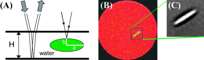
Figure 2: (color online) (A) Schematic of sample dimensions and the interference observation mode. (B) True interference color image of ellipsoid in the reflection mode of the microscope. (C) Bright field ellipsoid image in the transmission mode.

Particle motions observed by microscopy were recorded by a CCD camera to videotape at 30 frames/sec. In the dilute suspension, only one ellipsoid was visible in the $640\times 480~{}\textrm{pixel}^{2}=38.4\times 51.2~{}\mu\textrm{m}^{2}$ field of view under 100$\times$ objective during a half-hour experiment. We defocus slightly so that the ellipsoid can be more accurately located along its long axis. The built-in 2D Gaussian fit function in IDL (Interactive Data Language) was used to locate the center and orientation of the ellipse in each video frame. In practice, a small percent ($\sim$3%) of the frames failed to be correctly tracked. Without these frames, the trajectory breaks into short pieces and very long-time behavior becomes difficult to measure. To capture these frames, we very slightly adjusted tracking parameters or image contrast and re-analyzed the images; after these corrections roughly $3\%\times 3\%=0.09\%$ of the frames remain incorrectly tracked. We then repeated this procedure iteratively until all $\sim$50000 frames in one dataset were correctly tracked. The mean square displacements (MSD) at time lag $t=0$ has small non-zero intercept due to the tracking errors. Thus we can estimate the spatial and angular resolution from intercepts of their corresponding MSDs Crocker and Grier (1996). The orientation resolution is $1^{\circ}$, and spatial resolutions are 0.5 pixel = 40 nm along the particle’s short axis and 0.8 pixel = 64 nm along its long axis because of the superimposed small tumbling motion.

From the image analysis, we obtained the trajectory of a particle’s center-of-mass positions $\mathbf{x}(t_{n})=(x(t_{n}),y(t_{n}))$ in the lab frame and its orientation angle $\theta(t_{n})$ relative to the $x$-axis at times $t_{n}=n\times(1/30)$ sec, see Fig. 3. We define each $1/30$-sec time interval as a step. During the $n^{\rm th}$ step, the particle’s position changes by $\delta\mathbf{x}(t_{n})=\mathbf{x}(t_{n})-\mathbf{x}(t_{n-1})$ and its angle by $\delta\theta(t_{n})=\theta(t_{n})-\theta(t_{n-1})$. To obtain the drag coefficients along long and short axes, we need to covert the measured displacements from the fixed lab frame to the local body frame. Step displacements $\delta\tilde{\mathbf{x}}_{n}$ relative to the local body-frame and step displacements $\delta\mathbf{x}_{n}$ relative to the fixed lab frame are related via

$$\left(\begin{array}[]{c}\delta\tilde{x}_{n}\\ \delta\tilde{y}_{n}\end{array}\right)=\left(\begin{array}[]{cc}\cos\theta_{n}&\sin\theta_{n}\\ -\sin\theta_{n}&\cos\theta_{n}\end{array}\right)\left(\begin{array}[]{c}\delta x_{n}\\ \delta y_{n}\end{array}\right),$$ (5)

where $\theta_{n}=(\theta(t_{n-1})+\theta(t_{n}))/2$, see Fig. 3. In practice, choosing $\theta_{n}=\theta(t_{n-1})$ or $\theta_{n}=\theta(t_{n})$ has little effect on our results because $\theta$ barely changes during 1/30 s.

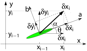
Figure 3: An ellipsoid in the $x$-$y$ lab frame and the $\tilde{x}$-$\tilde{y}$ body frame. The angle between two frames is $\theta(t)$. The displacement $\delta\mathbf{x}$ can be decomposed as ($\delta\tilde{x}$, $\delta\tilde{y}$) or ($\delta x$, $\delta y$).

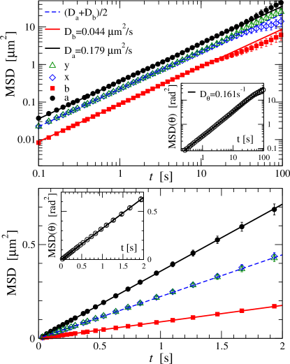
Figure 4: (color online) Mean square displacements (MSDs) of a $2.4\times 0.3\times 0.3~{}\mathrm{\mu m}^{3}$ ellipsoid confined in an $846~{}\mathrm{nm}$ thick cell. Top panel: log-log plot. Bottom panel: linear plot. The four lines arranged from top to bottom, respectively, are MSDs along $a$, $x$, $y$ and $b$ axes. Symbols represent experimental data, and lines represent linear fits to these data. Insets: Angular MSDs. All curves exhibit diffusive behavior, and the diffusion coefficients, $D=\textrm{MSD}/(2t)$, shown in the figure are derived from the best fit lines.

Figure 4 shows mean-square-displacements (MSDs) of a $2.4\times 0.3\times 0.3~{}\mathrm{\mu m}^{3}$ ellipsoid confined in an $846~{}\mathrm{nm}$ thick cell. In both the lab and the body frame, MSDs are diffusive with $\langle[\Delta\tilde{x}(t)]^{2}\rangle=2D_{a}t$, $\langle[\Delta\tilde{y}(t)]^{2}\rangle=2D_{b}t$, $\langle[\Delta x(t)]^{2}\rangle=\langle[\Delta y(t)]^{2}\rangle=(D_{a}+D_{b})t\equiv 2\overline{D}t$ and $\langle(\Delta\theta(t))^{2}\rangle=2D_{\theta}t$.

IV Results and Discussion

We repeated the experiments described above for different ellipsoids under different confinement conditions. From the slopes of their MSDs, we obtain $D_{a}$, $D_{b}$ and $D_{\theta}$ of different particles as a function of confinement condition as shown in Figs. 5,  6 and  7, respectively. Specifically, the normalized quantities, $D_{i}^{3D}/D_{i}=\gamma_{i}/\gamma^{3D}_{i}$, for $i=a,b,\theta$, are plotted as a function of increasing confinement, $2b/H$. Here the 3D normalization constants $D_{i}^{3D}$ (alternatively, $\gamma^{3D}_{i}$), are calculated from Eqs. 2 and 3.

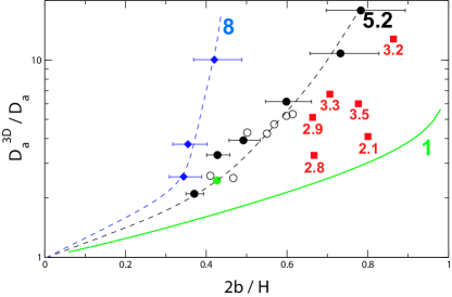
Figure 5: (color online) Ratio of theoretical 3D diffusion coefficient Happel and Brenner (1991) along the ellipsoid long axis, $D_{a}^{3D}$, to the measured diffusion coefficient, $D_{a}$, for ellipsoids confined at $2b/H$. Diamonds: $2.4\times 0.3\times 0.3~{}\mu$m³ ($\phi=8$) ellipsoids; Circles: $3.3\times 0.635\times 0.635~{}\mu$m³ ($\phi=5.2$) ellipsoids; Solid circles: From samples with no added salt; Open circles: From samples with 2 mM added salt; Green solid circle: From sample with BSA (bovine serum albumin) covered glass surfaces; Squares: All other samples - lower aspect ratio spheroids with particle aspect ratios labeled below each data point. The accuracy of $2b/H$ for these measurements is similar to other samples. Dashed curves: Guides for the eye. Solid curve ($\phi=1$): Replot of the numerical prediction in Fig. 1 of Ref. Bhattacharya et al. (2005) for a sphere strictly in the $H/2$ mid-plane.

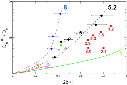
Figure 6: (color online) Ratio of theoretical 3D diffusion coefficient Happel and Brenner (1991) along the ellipsoid short axis, $D_{b}^{3D}$, to the measured diffusion coefficient, $D_{b}$, for ellipsoids confined at $2b/H$. Symbols are the same as those in Fig. 5. Solid curves from left to right: theoretical weak confinement predictions Happel and Brenner (1991) for aspect ratios $a/b=3,2$, and numerical result Bhattacharya et al. (2005) for aspect ration $a/b=1$ ranging over both weak and strong confinement regimes.

Notice that $2b/H=0$ corresponds to the 3D limit wherein $D^{3D}/D=1$. As expected, hydrodynamic drag increased and the diffusion coefficients correspondingly decrease as the confinement becomes stronger. The larger positive slopes exhibited by the more needle-like spheroids are indicative of motions more sensitive to confinement. Furthermore, the slopes of the same ellipsoids in Fig. 6 are larger than those in Fig. 5, indicating that diffusion along the ellipsoid short axis is more strongly affected by the confinement than diffusion along the long axis. Limited comparisons with all available analytical and numerical predictions (i.e. the solid curves in Figs. 5,  6), suggest that our data exhibit the generally expected trends with increasing confinement. Note that solid curves of analytical and numerical predictions in Figs. 5,  6 are for particles forced in the $z=H/2$ mid-plane. In real experiment, the measured drag is an average at different $z$. In our experiments, there are no detectable interference color changes at the centers of ellipsoids. Consequently $z$-fluctuations are less than $\sim 50~{}\mathrm{nm}\sim H/20$. In contrast, numerical results in Ref. Bhattacharya et al. (2005) show that the drag of a sphere at $H/3$ is very close ($<10$%) to the drag at $H/2$. Thus the $z$-fluctuations of our ellipsoids should have negligible effects on particle drags.

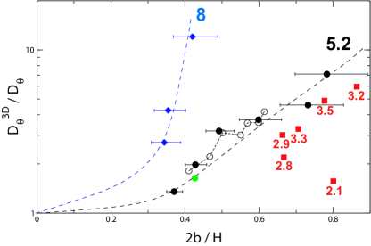
Figure 7: (color online) Ratio of theoretical rotational diffusion coefficient Perrin (1934); Koenig (1975) $D_{\theta}^{3D}$ to the measured diffusion coefficient, $D_{\theta}$, for ellipsoids confined at $2b/H$. Symbols are the same as those in Fig. 5.

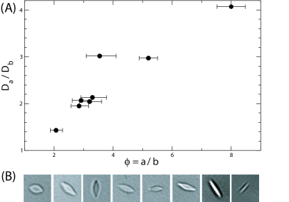
Figure 8: (A) Ratio of diffusion coefficients $D_{a}/D_{b}$ versus aspect ratio $\phi=a/b$. Seven of eight data points were taken for $2b/H\simeq 0.8$; the data point at $a/b=8$ was taken with $2b/H\simeq 0.4$. Solid curve: Theoretical result for $D_{a}/D_{b}$ versus aspect ratio $phi=$$a/b$ in 3D. (B) Microscope images of the corresponding eight particles as a function of aspect ratio (increasing from left to right). The dimensions of each particle from left to right: $[2a,2b]=[2.48,1.2]$, $[2.96,1.04]$, $[2.8,0.96]$, $[2.88,0.9]$, $[2.64,0.8]$, $[3.12,0.88]$, $[3.3,0.635]$, $[2.4,0.3]~{}\mu$m.

Another question that our data holds potential to explore concerns the effect of electric double layers on ellipsoid diffusion. The electric double layers around charged particles in suspension increase their hydrodynamic diameter and slow down diffusion, especially rotational diffusion because rotational drag is proportional to the volume rather than the length of the ellipsoid. This effect in rotational diffusion has been observed with depolarized dynamic light scattering in the regime where ionic concentration was low and spheroids small Matsuoka et al. (1996). In our systems such effects are expected to be small due to the high ionic strength of the suspension. As can be seen in Figs. 5, 6 and 7, diffusion coefficients are indistinguishable for the samples with 2 mM added salt and no added salt. The 6.9 nm screening layer of 2 mM solution lowers 3D diffusion coefficients by less than 2%.

Finally, Figure 8 shows the impact of aspect ratio on the ratio $D_{a}/D_{b}$. Here it is evident that diffusion in quasi-2D is quite different from diffusion in 3D. For 3D, $D_{a}/D_{b}$ asympotes to 2 at large aspect ratio, as shown by the solid theoretical curve. For quasi-2D, $D_{a}/D_{b}$, on the other hand, grows very rapidly with increasing aspect ratio Since we expect the stick boundary condition to hold in this system, the observation that $D_{a}/D_{b}=\gamma_{b}/\gamma_{a}>2$ should be purely due to confinement. A schematic to qualitatively capture this basic effect is given in Fig. 9. Imagine the fluid flowing past the ellipsoid. In 3D, the fluid flow pathways will be displaced by distances of order $2b$ in order to ‘go around’ the ellipsoid. This fluid flow displacement is the approximately the same, whether the spheroid is orientated either parallel or perpendicular to the flow, and therefore $\gamma_{a}$ and $\gamma_{b}$ are comparable. In 2D, however, the fluid flow pathway displacement is approximately $2b$ (or $2a$) when the spheroid is oriented parallel (perpendicular) to the flow, so that $\gamma_{b}/\gamma_{a}$ diverges with $a/b$. This qualitative picture also explains our observation that diffusion along the ellipsoid short axes is more strongly affected by the confinement than diffusion along the long axis. Finally, we note that in quasi-2D confinement, $D_{a}/D_{b}$ increases with increasing aspect ratio and should eventually saturate  Bhattacharya et al. (2005) at a value much larger than two, because some fluid will ‘leak’ between the particle and walls.

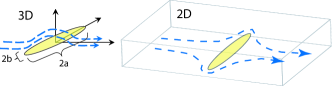
Figure 9: Schematic of fluid flow around an ellipsoid perpendicular to the flow. For the drag along short axes, fluid can flow around $2b$ in 3D, but has to flow around long axis $2a$ in 2D.

In summary, we have found that the anisotropic drag coefficients for ellipsoid diffusion substantially increase when the ellipsoids are strongly confined, especially along the short axes. In the future many questions remain about these systems will be exciting to explore, including the effects of neighboring ellipsoids and the effects of other confinement geometries. For example, quasi-1D confinement of an ellipsoid will align the ellipsoid along the diffusion direction. This effect may compensate the drag from boundaries and lead to an optimal diameter for ellipsoid diffusion speed in a quasi-1D cylinder.

V Acknowledgement

We thank Jerzy Blawzdziewicz for providing us with the theoretical curves at $\phi=1$ in Fig. 5 and 6. We also thank Tom Lubensky for useful conversations. This work was supported by the NSF-MRSEC grant #DMR-0520020 and partially by the NSF grant #DMR-0804881.

References

- Saffman and Delbruck (1975) P. G. Saffman and M. Delbruck, Proc. Natl. Acad. Sci. 72, 3111 (1975).
- Perrin (1934) F. Perrin, J. Phys. Radium V, 497 (1934).
- Perrin (1936) F. Perrin, J. Phys. Radium VII, 1 (1936).
- Happel and Brenner (1991) J. Happel and H. Brenner, Low Reynolds Number Hydrodynamics (Kluwer, Dordrecht, 1991).
- Bhattacharya et al. (2005) S. Bhattacharya, J. Blawzdziewicz, and E. Wajnryb, J. Fluid Mech. 541, 263 (2005).
- Lin et al. (2000) B. Lin, J. Yu, and S. A. Rice, Phys. Rev. E 62, 3909 (2000).
- Dufresne et al. (2001) E. R. Dufresne, D. Altman, and D. G. Grier, Europhys. Lett. 53, 264 (2001).
- Han et al. (2006) Y. Han, A. Alsayed, M. Nobili, J. Zhang, T. C. Lubensky, and A. G. Yodh, Science 314, 626 (2006).
- Mukhija and Solomon (2007) D. Mukhija and M. J. Solomon, J. Colloid Interface Sci. 314, 98 (2007).
- Kim et al. (2008) M. Kim, S. M. Anthony, and S. Granick, Soft Matter 5, 81 (2008).
- Bhaduri et al. (2008) B. Bhaduri, A. Neild, and T. W. Ng, Appl. Phys. Lett. 92, 084105 (2008).
- Koenig (1975) S. Koenig, Biopolymers 14, 2421 (1975).
- Hu and Zwanzig (1974) C. M. Hu and R. Zwanzig, J. Chem. Phys. 60, 4354 (1974).
- Bauer et al. (1974) D. R. Bauer, J. I. Brauman, and R. Pecora, J. Am. Chem. Soc. 96, 6840 (1974).
- Ho et al. (1993) C. C. Ho, A. Keller, J. A. Odell, and R. H. Ottewill, Colloid Polym. Sci. 271, 271 (1993).
- Crocker (1996) J. C. Crocker, Ph.D. thesis, The University of Chicago (1996).
- Hartshorne and Stuart (1970) N. H. Hartshorne and A. Stuart, Crystals and the Polarising Microscope (Edward Arnold Ltd., London, 1970).
- Crocker and Grier (1996) J. C. Crocker and D. G. Grier, J. Colloid Interface Sci. 179, 298 (1996).
- Matsuoka et al. (1996) H. Matsuoka, H. Morikawa, and H. Yamaoka, Colloids Surf., A 109, 137 (1996).