Solvation and Dissociation in Weakly Ionized Polyelectrolytes

Abstract

We present a Ginzburg-Landau theory of inhomogeneous polyelectrolytes with a polar solvent. First, we take into account the molecular (solvation) interaction among the ions, the charged monomers, the uncharged monomers, and the solvent molecules, together with the electrostatic interaction with a composition-dependent dielectric constant. Second, we treat the degree of ionization as a fluctuating variable dependent on the local electric potential. With these two ingredients included, our results are as follows. (i) We derive a mass reaction law and a general expression for the surface tension. (ii) We calculate the structure factor of the composition fluctuations as a function of various parameters of the molecular interactions, which provides a general criterion of the formation of mesophases. (iii) We numerically examine some typical examples of interfaces and mesophase structures, which strongly depend on the molecular interaction parameters.

I Introduction

Polyelectrolytes are much more complex than low-molecular-weight electrolytes and neutral polymers PG ; Barrat ; Rubinstein . Above all, the electrostatic interaction among the ionized monomers on the polymer chains and the mobile ions strongly influence the chain conformations and the mesophase formation Barrat ; Rubinstein ; Yoshikawa . Second, the dissociation (or ionization) on the chains should be treated as a chemical reaction in many polyelectrolytes containing weak acidic monomers Joanny ; Bu1 ; Bu2 , which is under the influence of the local electric potential. Then the degree of ionization is a space-dependent annealed variable in inhomogeneous polyelectrolytes, while it has mostly been treated to be a given constant in the theoretical literature. Such ionization heterogeneity should not be negligible in structure formations and in phase separation. Third, for water-like solvents with large dielectric constant $\varepsilon$, polymers are often hydrophobic and small ions are hydrophilic Bu1 , which can also affect the phase behavior. However, not enough attention has yet been paid on the effects of such short-range molecular interactions, where particularly relevant is the solvation (ion-dipole) interaction between ions and polar molecules Is .

In this paper we hence treat the degree of ionization as a fluctuating variable and include the molecular interactions. We show their relevance in polyelectrolytes in the simplest theoretical scheme. That is, we use the so-called random phase approximation PG in the Flory-Huggins scheme of weakly charged polyelectrolytes Lu1 ; Lu2 ; PD ; Krama . On the basis of a recent Ginzburg-Landau theory of ion distributions in binary mixtures Onuki-Kitamura ; OnukiPRE ; OnukiEPL ; OnukiW , we account for the solvation (hydration in aqueous solutions) between the charged particles (ions and ionized monomers) and the solvent molecules, whose free energy contribution usually much exceeds the thermal energy $T$ (per charged particle) Is . Hereafter we set the Boltzmann constant equal to unity.

In one-phase states of weakly charged polyelectrolytes, the structure factor $S(q)$ of the composition fluctuations with wave number $q$ was calculated in the random phase approximation Lu1 ; Lu2 , where the solvation interaction was neglected. Let $\phi$ and $f$ be the polymer volume fraction and the fraction of charged monomers on the chains, respectively. In this approximation the inverse of $S(q)$ is expressed as

$$\frac{1}{S(q)}={\bar{r}}(\phi)+\frac{q^{2}}{12a\phi(1-\phi)}+\frac{4\pi\ell_{B}f^{2}}{v_{0}^{2}(q^{2}+\kappa^{2})},$$ (1.1)

where the first term $\bar{r}$ depends on $\phi$ and $T$, $v_{0}=a^{3}$ is the volume of a monomer, $\ell_{B}=e^{2}/\epsilon T$ is the Bjerrum length, and $\kappa$ is the Debye-H$\ddot{\rm u}$ckel wave number. Due to the last electrostatic term in Eq.(1.1), $S(q)$ can have a peak at an intermediate wave number $q_{m}$ for small $\kappa$ or for low salt concentration. We here mention some related experiments. (i) Such a peak has been observed by scattering in one phase states of charged polymer systems Nishida ; Shibayama . It indicates formation of mesophases in sufficiently poor solvent, as was confirmed for a semidilue polyelectrolyte solution Candau . (ii) On the other hand, for neutral, polar binary mixturesOnuki-Kitamura ; OnukiPRE (or a mixture of neutral polymers and a polar solvent OnukiW ) with salt near the critical point, we calculated $S(q)$ in the same form as in Eq.(1.1). In electrolytes, the solvation interaction can strongly affect the composition fluctuations particularly near the critical point. In fact, in a recent scattering experiment Seto , a peak at an intermediate wave number has been observed in $S(q)$ in a near-critical binary mixture with salt. (iii) We also mention a finding of a broad peak in $S(q)$ in semi-dilute solutions of neutral polymers in a polar solvent with salt Hakim ; Hakim1 , where the solvation effect should be crucial. Thus we should calculate $S(q)$ in weakly charged polyelectrolytes including the solvation interaction.

We also mention calculations of the interface profiles in weakly charged polyelectrolytes in a poor solvent using the self-consistent field theory Shi ; Taniguchi . In these papers, however, the solvation interaction was neglected. In polyelectrolytes, the solvation interaction should decisively determine the charge distributions around an interface, as in electrolytes OnukiPRE ; OnukiW . In addition, the degree of ionization should significantly vary across an interface in polyelectrolytes, because the dissociation process strongly depends on the local counterion density.

The organization of this paper is as follows. In Section 2, we will present a Ginzburg-Landau approach accounting for the molecular interactions and the dissociation process. We will introduce the grand potential and present a theoretical expression for the surface tension. In Section 3, we will calculate the composition structure factor generalizing the results in the previous theories Onuki-Kitamura ; OnukiPRE ; Lu1 ; Lu2 . In Section 4, we will numerically examine the ion distributions around interfaces and in a periodic state.

II Theoretical background

We suppose weakly charged polymers in a theta or poor solvent consisting of a one-component polar fluid. We assume $f\ll 1$ to ensure flexibility of the chains. As suggested by Borue and ErukimovichLu1 and by Joanny and Leibler Lu2 , the random phase approximation can be used in concentrated solutions with

$$\phi>f^{2/3}(\ell_{B}/a)^{1/3}.$$ (2.1)

We consider the semidilute case $\phi>N^{-1/2}$, where $N$ is the polymerization index. Then the polymers consist of blobs with monomer number $g=\phi^{-2}$ and length $\xi_{b}=ag^{1/2}$ in the scaling theory PG and the electrostatic energy within a blob is estimated as

$$\epsilon_{b}=T(fg)^{2}\ell_{B}/\xi_{b}=Tf^{2}\phi^{-3}\ell_{B}a^{-1}.$$ (2.2)

Here the salt density is assumed not to exceed the density of the charged monomers $n_{p}$. Obviously, the condition $\epsilon_{b}<T$ yields Eq.(2.1). In our case the Debye-H$\ddot{\rm u}$ckel wave number $\kappa\propto(n_{p}\ell_{B})^{1/2}$ is sufficiently small such that $n_{p}\gg\kappa^{3}$ holds and a free energy contribution due to the charge density fluctuations $\propto\kappa^{3}$ is negligible Landau ; Onukibook .

II.1 Ginzburg-Landau free energy

For weakly ionized polyelectrolytes, we set up the free energy accounting for the molecular interactions and the ionization equilibrium. We neglect the image interaction Rubinstein ; OnukiPRE ; Onsager and the formation of dipole pairs and ion clusters pair ; Krama . The former is important across an interface when the dielectric constants of the two phases are distinctly different in the dilute limit of the ion densities (see comments in the last section), while the latter comes into play at not small ion densities.

The volume fractions of the polymer and the solvent are written as $\phi({\mbox{\boldmath$r$}})$ and $1-\phi({\mbox{\boldmath$r$}}),$ respectively. For simplicity, we neglect the volume fractions of the ions and assume that the monomers and the solvent molecules have a common volume $v_{0}=a^{3}$. Then $\phi$ is also the molar composition. The counterion density is written as $n_{c}({\mbox{\boldmath$r$}})$. We may add salt with cation and anion densities $n_{1}({\mbox{\boldmath$r$}})$ and $n_{2}({\mbox{\boldmath$r$}})$, respectively. The ion charges are $Z_{i}$ with $i=c,1$, and 2. In the monovalent case, for example, we have $Z_{c}=1$, $Z_{1}=1$, and $Z_{2}=-1$, respectively. In the continuum limit these variables are smooth coarse-grained ones on the microscopic level.

The number of the ionizable monomers on a chain is $\nu_{M}N$ with $\nu_{M}<1$. In this work the degree of ionization $\zeta({\mbox{\boldmath$r$}})$ in the range $0\leq\zeta\leq 1$ depends on the surrounding conditions and is inhomogeneous. Then the fraction of ionized monomers is

$$f=\nu_{M}\zeta,$$ (2.3)

and the number density of ionized monomers is

$$n_{p}=v_{0}^{-1}f\phi=v_{0}^{-1}\nu_{M}\zeta\phi,$$ (2.4)

where $\zeta$ and $\phi$ are space-dependent. The condition of weak ionization $f\ll 1$ is always satisfied for $\nu_{M}\ll 1$, but we need to require $\zeta\ll 1$ for $\nu_{M}\sim 1$. Furthermore, we assume that the charge of each ionized group is negative and monovalent (or equal to $-e$) so that the total charge density is written as

$$\rho=e\sum_{i=c,1,2}Z_{i}n_{i}-en_{p}.$$ (2.5)

The overall charge neutrality condition is $\int d{\mbox{\boldmath$r$}}\rho=0$. In more detail in the present of salt, we have

$$\int d{\mbox{\boldmath$r$}}[Z_{c}n_{c}-n_{p}]=\int d{\mbox{\boldmath$r$}}[Z_{1}n_{1}+Z_{2}n_{2}]=0.$$ (2.6)

The free energy $F$ of our system is the space integral of a free energy density $f_{T}$ in the fluid container. We assume that $f_{T}$ is of the form,

$$f_{T} = f_{0}(\phi,T)+\frac{T}{2}C(\phi)|\nabla\phi|^{2}+\frac{\varepsilon(\phi)}{8\pi}{{\mbox{\boldmath$E$}}}^{2}$$ (2.7)

$$+T\sum_{i=c,1,2}{n_{i}}[\ln(n_{i}v_{0})-1+g_{i}\phi]+T(\Delta_{0}+g_{p}\phi)n_{p}$$

$$+Tv_{0}^{-1}\nu_{M}\phi[\zeta\ln\zeta+(1-\zeta)\ln(1-\zeta)].$$

In the first line, the first term $f_{0}$ is the chemical part in the Flory-Huggins form PG ; Onukibook ,

$$f_{0}=\frac{T}{v_{0}}[\frac{\phi}{N}\ln\phi+(1-\phi)\ln(1-\phi)+\chi\phi(1-\phi)],$$ (2.8)

where $\chi$ is the interaction parameter dependent on the temperature $T$ and its critical value is $\chi_{c}=(1+N^{-1/2})^{2}/2$. in the absence of ions. The second term is the gradient part with the composition-dependent coefficient PG ,

$$C(\phi)=1/12a\phi(1-\phi),$$ (2.9)

where $a=v_{0}^{1/3}$. The third term is the electrostatic free energy, where ${\mbox{\boldmath$E$}}=-\nabla\Phi$ is the electric field. The electrostatic potential $\Phi$ satisfies the Poisson equation,

$$\nabla\cdot\varepsilon(\phi)\nabla\Phi=-4\pi\rho.$$ (2.10)

The dielectric constant $\varepsilon(\phi)$ changes from the solvent value $\varepsilon_{0}$ to the polymer value $\varepsilon_{p}$ with increasing $\phi$. For simplicity, we assume the linear form,

$$\varepsilon(\phi)=\varepsilon_{0}+\varepsilon_{1}\phi,$$ (2.11)

where $\varepsilon_{1}=\varepsilon_{p}-\varepsilon_{0}$. In some binary fluid mixtures, the linear form of $\varepsilon(\phi)$ has been measured Debye-Kleboth . For charged gels, Kramarenko et al. pointed out relevance of strong composition-dependence of $\varepsilon(\phi)$ in first-order swelling transition gel . In the second line of Eq.(2.7), the coupling terms $Tg_{i}\phi n_{i}$ ($i=c,1,2,p$) arise from the molecular interactions among the charged and uncharged particles, while $T\Delta_{0}$ is the dissociation energy in the dilute limit $\phi\to 0$. In the third line of Eq.(2.7), we give the entropic free energy of dissociationJoanny ; Bu1 ; Bu2 , where $v_{0}^{-1}\nu_{M}\phi$ is the density of the ionizable monomers.

Solvation interaction. We have introduced the molecular interaction terms ($\propto g_{i}$), which will be simply called the solvation interaction terms. In low-molecular-weight binary mixtures with salt Onuki-Kitamura ; OnukiPRE , such terms arise from the composition-dependence of the solvation chemical potential of ions $\mu_{i}^{\rm sol}$, where $i$ represents the ion species. The original Born theory Born gave $\mu_{i}^{\rm sol}=Z_{i}^{2}e^{2}/2\varepsilon(\phi)R_{i}$, where $Z_{i}e$ is the ion charge and $R_{i}$ is called the Born radius. Here $R_{i}$ is of order $1{\rm\AA}$ for small metallic ions in aqueous solution Is . For each ion species, the difference of $\mu_{i}^{\rm sol}$ in the coexisting two phases is the Gibbs transfer free energy typically much larger than $T$ per ion ($\sim 15T$ for monovalent ions) in electrochemistry Hung ; Osakai . In polymer solutions, the origin of these terms can be more complex Hakim ; Hakim1 ; Hydrogen . For example, ions interact with the dipoles of the solvent molecules and those on the chains differently, affecting the hydrogen bonding around the chains. Therefore, the solvation chemical potential of an charged particle of the species $i$ ($i=c,1,2,p$) arises from the interaction with the solvent molecules and that with the uncharged monomers as

$$\mu_{i}^{\rm sol}=\epsilon_{i}^{s}(1-\phi)+\epsilon_{i}^{m}\phi=(\epsilon_{i}^{m}-\epsilon_{i}^{s})\phi+\epsilon_{i}^{s},$$ (2.12)

where $\epsilon_{i}^{m}$ and $\epsilon_{i}^{s}$ are the interaction energies. The solvation contribution to the free energy is given by the space integral of the sum,

$$\sum_{i}\mu_{i}^{\rm sol}n_{i}=T\sum_{i}g_{i}\phi n_{i}+\sum_{i}\epsilon_{i}^{s}n_{i}.$$ (2.13)

Here we find $g_{i}$ appearing in Eq.(2.7) expressed as

$$g_{i}=(\epsilon_{i}^{m}-\epsilon_{i}^{s})/T.$$ (2.14)

The last term on the right hand side of Eq.(2.12) contributes to a constant (irrelevant) chemical potential for $i=1,2$ and to the constant $\Delta_{0}$ in Eq.(2.7) for $i=c,p$ (with the aid of Eq.(2.6) for $i=c$). As a result, we have attraction for $g_{i}<0$ and repulsion for $g_{i}>0$ between the ions ($i=c,1,2$) and the polymer chains, while we have a composition-dependent dissociation constant from $i=c,p$ (see Eq.(2.27)). For water-like solvent, $g_{i}>0$ for hydrophilic ions and $g_{i}<0$ for hydrophobic ions. The Born theory Born and the data of the Gibbs transfer free energy Hung ; Osakai both suggest that $|g_{i}|$ mostly much exceeds unity and is even larger for multivalent ions such as Ca²⁺.

II.2 Equilibrium relations

As a typical experimental geometry, our fluid system is inserted between two parallel metal plates with area $S$ and separation distance $L$(much shorter than the lateral dimension $S^{1/2}$). If the surface charge densities at the upper and lower plates are fixed at $\pm\sigma_{0}$, the electrostatic energy $F_{e}=\int d{\mbox{\boldmath$r$}}{\varepsilon(\phi)}{{\mbox{\boldmath$E$}}}^{2}/{8\pi}$ is a functional of $\phi$ and $\rho$. The potential values at the two plates are laterally homogeneous, but are fluctuating quantities OnukiPRE .

For small variations $\delta\phi$ and $\delta\rho$ superimposed on $\phi$ and $\rho$, the incremental change of $F_{e}$ is written as OnukiPRE

$$\delta F_{e}=\int d{\mbox{\boldmath$r$}}\bigg{[}\Phi\delta\rho-\frac{\varepsilon_{1}{\mbox{\boldmath$E$}}^{2}}{8\pi}\delta\phi\bigg{]}.$$ (2.15)

Under the charge neutrality $\int d{\mbox{\boldmath$r$}}\rho=0$, we first minimize $F$ with respect to $\zeta$ (or $n_{p}$) and $n_{c}$ at fixed $n_{1}$, $n_{2}$, and $\phi$. It is convenient to introduce $G=F+(T\lambda/e)\int d{\mbox{\boldmath$r$}}\rho$, where $T\lambda/e$ is the Lagrange multiplier independent of space. Using Eq.(2.15) we may calculate ${\delta G}/{\delta\zeta}$ and ${\delta G}/{\delta n_{c}}$. Setting them equal to zero, we obtain

$$\frac{\zeta}{1-\zeta}=\exp[U+\lambda-\Delta_{0}-g_{p}\phi],$$ (2.16)

$$n_{c}=v_{0}^{-1}\exp[-U-\lambda-g_{c}\phi],$$ (2.17)

where we introduce the normalized electric potential by

$$U={e}\Phi/T.$$ (2.18)

Next, homogeneity of the ion chemical potentials $\mu_{i}=\delta F/\delta n_{i}$ ($i=1,2)$ yields

$$n_{i}=n_{i}^{0}\exp[-g_{i}\phi-Z_{i}(U+\lambda)],$$ (2.19)

where $n_{i}^{0}=v_{0}^{-1}e^{\mu_{i}/T}$ are constants. Here $U$ and $\lambda$ appear in the combination $U+\lambda$ in all the physical quantities. If $U+\lambda$ is redefined as $U$, $\lambda$ may be set equal to zero without loss of generality.

We also require homogeneity of $h=\delta F/\delta\phi$, where we fix $n_{c},n_{1},n_{2}$ and $n_{p}$ in the functional derivative. With the aid of Eq.(2.15) some calculations give

$$\frac{h}{T} = \frac{1}{T}f_{0}^{\prime}(\phi)+\frac{C^{\prime}}{2}|\nabla\phi|^{2}-\nabla\cdot C\nabla\phi-\frac{\varepsilon_{1}}{8\pi T}{E}^{2}$$ (2.20)

$$+\sum_{i=c,1,2,p}g_{i}n_{i}+v_{0}^{-1}\nu_{M}\ln(1-\zeta),$$

where $f_{0}^{\prime}={\partial f_{0}}/{\partial\phi}$ and $C^{\prime}=\partial C/\partial\phi$. On the right hand side, the first three terms are those in the usual Ginzburg-Landau theory Onukibook . The last three terms arise from the electrostatic interaction, the solvation interaction, and the dissociation equilibration, respectively. We may calculate the interface profiles and the mesophase profiles from the homogeneity of $h$ OnukiPRE .

Surface tension. In the above procedure, we have minimized the grand potential $\Omega=\int d{\mbox{\boldmath$r$}}\omega$ under the charge neutrality $\int d{\mbox{\boldmath$r$}}\rho=0$, where the grand potential density is defined by

$$\omega=f_{T}-h\phi-\mu_{1}n_{1}-\mu_{2}n_{2},$$ (2.21)

with $f_{T}$ being given by Eq.(2.7). Using Eqs. (2.16)-(2.19) we may eliminate $\mu_{1}$ and $\mu_{2}$ to obtain

$$\omega = f_{0}+\frac{TC}{2}|\nabla\phi|^{2}-h\phi+\frac{\varepsilon}{8\pi}{{\mbox{\boldmath$E$}}}^{2}-\rho\Phi$$ (2.22)

$$-T\sum_{i=c,1,2}{n_{i}}+Tv_{0}^{-1}\nu_{M}\phi\ln(1-\zeta).$$

Furthermore, using Eq.(2.20) we may calculate the space gradient of $\omega$ as

$$\frac{\partial\omega}{\partial x_{k}}=\sum_{\ell}\frac{\partial}{\partial x_{\ell}}\bigg{(}{TC}\frac{\partial\phi}{\partial x_{k}}\frac{\partial\phi}{\partial x_{\ell}}\bigg{)}-\frac{\partial}{\partial x_{k}}\rho U,$$ (2.23)

where $\partial/\partial x_{k}$ and $\partial/\partial x_{\ell}$ are the space derivatives with respect to the Cartesian coordinates $x,y$, and $z$. In the one-dimensional case, where all the quantities vary along the $z$ axis, the above equation is integrated to give

$$\omega=TC(\phi^{\prime})^{2}-\rho\Phi+\omega_{\infty},$$ (2.24)

where $\phi^{\prime}=d\phi/dz$ and $\omega_{\infty}$ is a constant. Therefore, around a planar interface separating two bulk phases, $\omega(z)$ tends to a common constant $\omega_{\infty}$ as $z\to\pm\infty$. From the above relation the surface tension $\gamma=\int dz[\omega(z)-\omega_{\infty}]$ is expressed as

$$\frac{\gamma}{T} = 2\int dz\bigg{[}\frac{\hat{f}_{0}}{T}-\sum_{i=c,1,2}{n_{i}}+\frac{\nu_{M}\phi}{v_{0}}\ln(1-\zeta)\bigg{]}$$ (2.25)

$$= \int dz\bigg{[}C(\phi^{\prime})^{2}-\frac{\varepsilon(\phi)}{4\pi T}{\mbox{\boldmath$E$}}^{2}\bigg{]},$$

where $\hat{f_{0}}=f_{0}-h\phi-\omega_{\infty}$ in the first line and use is made of $\int dz\rho\Phi=\int dz\varepsilon{\mbox{\boldmath$E$}}^{2}/4\pi$. In the second line the integrand consists of a positive gradient term and a negative electrostatic term. Similar expressions for the surface tension have been obtained for electrolytes OnukiPRE and ionic surfactant systems OnukiEPL .

Mass action law. If Eqs.(2.12) and (2.13) are multiplied, $U$ cancels to disappear. It follows the equation of ionization equilibrium or the mass action equation Bu1 ; Bu2 ,

$$\frac{\zeta}{1-\zeta}n_{c}=K(\phi),$$ (2.26)

where $K(\phi)$ is the dissociation constant of the form,

$$K(\phi)=v_{0}^{-1}\exp[-\Delta_{0}-(g_{p}+g_{c})\phi].$$ (2.27)

We may interpret $\Delta(\phi)\equiv\Delta_{0}+(g_{p}+g_{c})\phi$ as the composition-dependent dissociation energy divided by $T$. With increasing $\phi$, the dissociation decreases for positive $g_{p}+g_{c}$ and increases for negative $g_{p}+g_{c}$. If $g_{p}+g_{c}\gg 1$, $K(\phi)$ much decreases even for a small increase of $\phi$. Then $\zeta$ and $n_{p}$ are related to $n_{c}$ as

$$\zeta=\frac{v_{0}n_{p}}{\nu_{M}\phi}=\frac{K}{K+n_{c}}.$$ (2.28)

These relations hold in equilibrium states, which may be inhomogeneous. In our theory, $n_{p}=n_{p}(\phi,U)$ is a function of the local values of $\phi$ and $U$ as well as $n_{c}$, $n_{1}$, and $n_{2}$. Here,

$$\frac{\partial n_{p}}{\partial U}=(1-\zeta)n_{p},\quad\frac{\partial n_{p}}{\partial\phi}=\frac{n_{p}}{\phi}-(1-\zeta)g_{p}n_{p},$$ (2.29)

so $n_{p}$ increases with increasing $U$ at fixed $\phi$.

Relations in bulk without salt. Furthermore, in a homogeneous bulk phase with $n_{p}=n_{c}$, Eq.(2.28) yields the quadratic equation for $n_{c}$,

$$n_{c}({n_{c}+K})=v_{0}^{-1}\nu_{M}\phi K,$$ (2.30)

which is solved to give

$$\zeta=\frac{v_{0}n_{c}}{\nu_{M}\phi}=\frac{2}{\sqrt{Q+1}+1}.$$ (2.31)

Here it is convenient to introduce

$$Q(\phi)={4\nu_{M}\phi}/{v_{0}K(\phi)}.$$ (2.32)

In particular, we find $\zeta\ll 1$ and $n_{c}\cong(\nu_{M}\phi K/v_{0})^{1/2}$ for $Q\gg 1$, while $\zeta\rightarrow 1$ for $Q\ll 1$. Thus the ion density $n_{c}$ has been determined for given $\phi$.

Relations in bulk with salt. As another simple situation, we may add a salt whose cations are of the same species as the counterions. The cations and anions are both monovalent. Here the counterionsa and the cations from the salt are indistinguishable. Thus the sum of the counterion density $n_{c}$ and the salt cation density $n_{1}$ is written as $n_{c}$, while the salt anion density is written as $n_{2}$. The charge neutrality condition becomes $n_{c}=n_{p}+n_{2}$ in the bulk. From Eq.(2.28) we obtain

$$n_{c}=v_{0}^{-1}{\nu_{M}\phi}K/(K+n_{c})+n_{2},$$ (2.33)

in the bulk phase. Then $n_{c}$ increases with increasing $n_{2}$. We treat $n_{2}$ as an externally given constant to obtain

$$n_{c} = \frac{1}{2}(n_{2}-K)+\frac{1}{2}\sqrt{(n_{2}+K)^{2}+4v_{0}^{-1}\nu_{M}\phi K}$$ (2.34)

$$\cong n_{2}+v_{0}^{-1}\nu_{M}\phi K/(n_{2}+K),$$

where the second line holds in the case $n_{2}+K\gg 2(\nu_{M}\phi K/v_{0})^{1/2}=Q^{1/2}K$. With increasing $n_{2}$, the ionized monomer density $n_{p}=n_{c}-n_{2}$ decreases, while $n_{c}$ increases. At high salt densities, where $n_{2}$ much exceeds both $2(\nu_{M}\phi K/v_{0})^{1/2}$ and $K$, we eventually obtain

$$n_{c}\cong n_{2},\quad n_{p}\cong\nu_{M}\frac{K\phi}{n_{2}}\ll n_{2},\quad\zeta\cong\frac{K}{n_{2}}\ll 1.$$ (2.35)

III Structure Factor of Composition Fluctuations

In phase transition theories Onukibook the order parameter fluctuations obey the equilibrium distribution $\propto\exp(-F/T)$, where $F$ is the Ginzburg-Landau free energy functional. In the present problem, the thermal flucuations of $\phi$, $n_{i}$, and $\zeta$ are assumed to obey the distribution $\propto\exp(-F/T)$ in equilibrium, where $F$ is the space integral of $f_{T}$ in Eq.(2.7). In the Gaussian approximation of $F$, we consider small plane-wave fluctuations of $\phi$, $n_{i}$, and $\zeta$ with wave vector $q$ in a one-phase state. It then follows the mean-field expression for the structure factor $S(q)$ of the composition fluctuations. It is of the form of Eq.(1.1) for a constant degree of ionization $\zeta$ in the absence of the solvation interaction. Here it will be calculated including the solvation interaction and in the annealed case. We examine how it depends on the parameters $g_{c}$, $g_{1}$, $g_{2}$, and $g_{p}$ and how it is modified by the fluctuating ionization.

III.1 Gaussian approximation

From Eq.(2.7) the fluctuation contributions to $F$ in the bilinear order are written as

$$\frac{\delta F}{T} = \sum_{\mbox{\boldmath$q$}}\bigg{[}\frac{1}{2}({{\bar{r}}+Cq^{2}})|\phi_{\small{\mbox{\boldmath$q$}}}|^{2}+\frac{2\pi}{\varepsilon q^{2}}|\rho_{\small{\mbox{\boldmath$q$}}}|^{2}+\sum_{i=c,1,2}\frac{|n_{i{\small{\mbox{\boldmath$q$}}}}|^{2}}{2{n_{i}}}$$ (3.1)

$$+\sum_{i=c,1,2,p}g_{i}n_{i{\small{\mbox{\boldmath$q$}}}}\phi_{\small{\mbox{\boldmath$q$}}}^{*}+\frac{n_{p}}{2(1-\zeta)\zeta^{2}}|\zeta_{\small{\mbox{\boldmath$q$}}}|^{2}\bigg{]},$$

where $\phi_{\small{\mbox{\boldmath$q$}}}$, $\rho_{\small{\mbox{\boldmath$q$}}}$, $n_{i{\small{\mbox{\boldmath$q$}}}}$ ($i=c,1,2,p)$, and $\zeta_{\small{\mbox{\boldmath$q$}}}$ are the Fourier components of $\phi({\mbox{\boldmath$r$}})$, $\rho({\mbox{\boldmath$r$}})$, $n_{i}({\mbox{\boldmath$r$}})$, and $\zeta({\mbox{\boldmath$r$}})$, respectively. From Eq.(2.4) the fluctuation of the charged-monomer density is of the form,

$$n_{p{\small{\mbox{\boldmath$q$}}}}=\frac{n_{p}}{\zeta}\zeta_{{\small{\mbox{\boldmath$q$}}}}+\frac{n_{p}}{\phi}\phi_{{\small{\mbox{\boldmath$q$}}}}.$$ (3.2)

In this section $\phi$ and $n_{i}$ denote the spatial averages, where $n_{p}=\sum_{i=c,1,2}Z_{i}n_{i}$ from the overall charge neutrality. The inhomogeneity in the dielectric constant may be neglected for small fluctuations. From the Flory-Huggins free energy (2.8) the coefficient $\bar{r}$ is of the form,

$$v_{0}{\bar{r}}=\frac{v_{0}}{T}\frac{\partial^{2}f_{0}}{\partial\phi^{2}}=\frac{1}{N\phi}+\frac{1}{1-\phi}-2\chi.$$ (3.3)

On the right and side of Eq.(3.1), the first term yields the Ornstein-Zernike structure factor of the composition without the coupling to the charged particles. The second and third terms are well-known for electrolyte systems, leading to the Debye-H$\ddot{\rm u}$ckel screening of the charge density correlation. The fourth term arises from the solvation interaction, while the fifth term from the fluctuation of ionization.

We minimize $\delta F$ with respect to $n_{i{\small{\mbox{\boldmath$q$}}}}$ ($i=c,1,2,p)$ at fixed $\phi_{{\small{\mbox{\boldmath$q$}}}}$ to express them in the linear form $n_{i{\small{\mbox{\boldmath$q$}}}}\propto\phi_{{\small{\mbox{\boldmath$q$}}}}$. In particular, $\rho_{{\small{\mbox{\boldmath$q$}}}}$ and $\zeta_{{\small{\mbox{\boldmath$q$}}}}$ are written as

$$\rho_{{\small{\mbox{\boldmath$q$}}}} = \frac{q^{2}}{4\pi\ell_{B}}U_{{\small{\mbox{\boldmath$q$}}}}=-\frac{Aq^{2}}{q^{2}+\kappa_{T}^{2}}\phi_{{\small{\mbox{\boldmath$q$}}}},$$ (3.4)

$$\zeta_{{\small{\mbox{\boldmath$q$}}}} = -\zeta(1-\zeta)\bigg{[}g_{p}+\frac{4\pi\ell_{B}A}{q^{2}+\kappa_{T}^{2}}\bigg{]}\phi_{{\small{\mbox{\boldmath$q$}}}},$$ (3.5)

where $U_{{\small{\mbox{\boldmath$q$}}}}$ is the Fourier component of $U({\mbox{\boldmath$r$}})$, and

$$\kappa_{T}^{2}=4\pi\ell_{B}[(1-\zeta)n_{p}+\sum_{i=c,1,2}Z_{i}^{2}n_{i}],$$ (3.6)

$$A=\frac{n_{p}}{\phi}-(1-\zeta)g_{p}n_{p}+\sum_{i=c,1,2}Z_{i}g_{i}n_{i}.$$ (3.7)

Here $\kappa_{T}$ defined in Eq.(3.6) is a generalized Debye-H$\ddot{\rm u}$ckel wave number introduced by Raphael and Joanny Joanny , where the term proportional to $n_{p}$ arises from dissociation and recombination on the polymer chains. The first relation (3.4) itself readily follows from the relations,

$$\frac{\partial\rho}{\partial\phi}=-eA,\quad\frac{\partial\rho}{\partial U}=-\frac{e\kappa_{T}^{2}}{4\pi\ell_{B}},$$ (3.8)

where $\rho({\mbox{\boldmath$r$}})$ is regarded as a function of the local values of $U({\mbox{\boldmath$r$}})$ and $\phi({\mbox{\boldmath$r$}})$ as discussed around Eqs.(2.28) and (2.29). From Eq.(3.5) we find $\zeta_{{\small{\mbox{\boldmath$q$}}}}\rightarrow 0$ as $\zeta\to 0$ or 1. We can see that the last term on the right hand side of Eq.(3.1) is negligible as $\zeta\to 1$.

After elimination of $n_{i{\small{\mbox{\boldmath$q$}}}}$ ($i=c,1,2,p)$ the free energy change $\delta F$ is expressed as $\delta F=\sum_{\mbox{\boldmath$q$}}T|\phi_{\small{\mbox{\boldmath$q$}}}|^{2}/S(q)$, where $S(q)$ is the composition structure factor calculated as

$$\frac{1}{S(q)} = {\bar{r}}+r_{s}+Cq^{2}+\frac{4\pi\ell_{B}A^{2}}{q^{2}+\kappa_{T}^{2}}$$ (3.9)

$$={\bar{r}}+r_{s}+C\gamma_{p}^{2}\kappa_{T}^{2}+Cq^{2}\bigg{[}1-\frac{\gamma_{p}^{2}\kappa_{T}^{2}}{q^{2}+\kappa_{T}^{2}}\bigg{]},$$

where $r_{s}$ is the shift of $\bar{r}$ arising from the solvation interaction given by

$$r_{s}=[{2}{\phi}^{-1}g_{p}-(1-\zeta)g_{p}^{2}]n_{p}-\sum_{i=c,1,2}g_{i}^{2}n_{i}.$$ (3.10)

As $\phi\to 0$ we have $r_{s}\cong 2g_{p}f$. For large $|g_{i}|\gg 1$ the other negative terms ($\propto g_{1}^{2}$) can be significant, leading to $r_{s}<0$. In the second line of Eq.(3.9) $\gamma_{p}$ is defined by

$$\gamma_{p}=\sqrt{\frac{4\pi\ell_{B}}{C}}\frac{A}{\kappa_{T}^{2}}=\frac{(4\pi\ell_{B}C)^{-1/2}A}{(1-\zeta)n_{p}+\sum_{i=c,1,2}Z_{i}^{2}n_{i}},$$ (3.11)

where $(4\pi\ell_{B}C)^{-1/2}=[3a\phi(1-\phi)/\pi\ell_{B}]^{1/2}$ if use is made of Eq.(2.9). Note that $r_{s}$ and $\kappa_{T}^{2}$ consist of the terms proportional to the charge densities, while $\gamma_{p}$ depends on their ratios. In particular, if $n_{c}=n_{p}$ and $n_{1}=n_{2}$ in the monovalent case, $\gamma_{p}$ depends on the density ratio $R\equiv n_{1}/n_{p}$ as

$$\gamma_{p}=\frac{(4\pi\ell_{B}C)^{-1/2}}{{2-\zeta+2R}}\bigg{[}\frac{1}{\phi}-(1-\zeta)g_{p}+g_{c}+(g_{1}-g_{2})R\bigg{]}.$$ (3.12)

Here $R=0$ for salt-free polyelectrolytes and $R$ is increased with increasing the salt density. As $R\to\infty$ the above formula tends to that for neutral polymer solutions (low-molecular-weight binary mixtures for $N=1$) with salt. We note that $\gamma_{p}$ can even be negative depending on the solvation terms in the brackets on the right hand side of Eq.(3.12).

III.2 Macrophase and microphase separation

From the second line of Eq.(3.9) we obtain the small-$q$ expansion $S(q)^{-1}=a_{0}+a_{1}q^{2}+a_{2}q^{4}\cdots$ with

$$a_{1}=C(1-\gamma_{p}^{2}),$$ (3.13)

so we encounter the following two cases. (i) If $|\gamma_{\rm p}|<1$, $S(q)$ is maximum at $q=0$ and we predict the usual phase transition with increasing $\chi$ in the mean field theory. The spinodal $\chi=\chi_{\rm sp}$ is given by

$$2\chi_{\rm sp}=\frac{1}{N\phi}+\frac{1}{1-\phi}+r_{s}+C\gamma_{p}^{2}\kappa_{T}^{2}.$$ (3.14)

Macroscopic phase separation occurs for $\chi>\chi_{\rm sp}$. On the right hand side of Eq.(3.14), $r_{s}=0$ and the last term becomes $n_{p}/(1-\zeta)\phi^{2}>0$ for $g_{i}=0$, but the sum of the last two terms can be much altered for $|g_{i}|\phi\gtrsim 1$. For example, without salt and in the monovalent case, it is equal to $[1/\phi^{2}+\zeta g_{c}^{2}+2g_{c}/\phi]n_{p}/(1-\zeta)-2g_{p}g_{c}n_{p}$. (ii) If $|\gamma_{\rm p}|>1$, $S(q)$ has a peak at an intermediate wave number $q_{m}$ given by

$$q_{m}^{2} = (4\pi\ell_{B}/C)^{1/2}|A|-\kappa_{T}^{2}$$ (3.15)

$$= \kappa_{T}^{2}(|\gamma_{p}|-1).$$

Thus $q_{m}\to 0$ as $\kappa_{T}\to 0$ or as $|\gamma_{p}|\to 1$. The spinodal is given by $S(q_{m})^{-1}=0$ or by

$$2\chi_{\rm sp}=\frac{1}{N\phi}+\frac{1}{1-\phi}+r_{s}+C\kappa_{T}^{2}(2|\gamma_{p}|-1).$$ (3.16)

Microphase separation should be triggered for $\chi>\chi_{\rm sp}$. Since $\gamma_{p}$ depends only on the ion density ratio $R$ as in Eq.(3.12), the criterion $\gamma_{p}>1$ remains unchanged however small the densities of the charged particles are. Of course, mesophase formation is well-defined only when $q_{m}$ in Eq.(3.15) is much larger than the inverse of the system length. In the following we discuss some special cases.

Polyelectrolytes without solvation interaction. For $g_{i}=0$, we have $r_{s}=0$ and $A=n_{p}/\phi=v_{0}^{-1}f$ as in the previous theories of weakly ionized polyelectrolytes Lu1 ; Lu2 ; Joanny . In the monovalent case Eq.(3.12) gives

$$\gamma_{p} = 1/[(4\pi\ell_{B}C)^{1/2}{(2-\zeta+2R)\phi}]$$ (3.17)

$$= [3a\phi/\pi\ell_{B}(1-\phi)]^{1/2}/(2-\zeta+2R),$$

where $R=n_{1}/n_{p}$ and use is made of Eq.(2.9) in the second line. Here $\gamma_{p}$ is largest without salt ($R=0$) and decreases with increasing $R$. In accord with this predicted salt effect, Braun et al. Candau observed a mesophase at low salt concentration and a macroscopic phase separation at high salt concentration. However, for large $|g_{i}|$, the solvation interaction comes into play. Thus more experiments are desirable to detect it in polyelectrolytes with water-like solvent.

Binary mixtures with solvation interaction. Without ionization or for $f=0$, we have $n_{p}=n_{c}=0$. Here we describe a neutral binary mixture with salt. Further for a monovalent salt, we have $A=(g_{1}-g_{2})n_{1}$ and

$$\gamma_{p} = (g_{1}-g_{2})/(16\pi\ell_{B}C)^{1/2},$$ (3.18)

$$r_{s} = -(g_{1}^{2}+g_{2}^{2})n_{1}.$$ (3.19)

From neutron scattering, Sadakane et al.Seto found periodic structures in a near-critical, low-molecular-weight mixture of D₂O and trimethylpyridine (3MP) containing sodium tetrarphenylborate (NaBPh₄). Their salt is composed of strongly hydrophilic cation Na⁺ and strongly hydrophobic anion BPh${{}_{4}}^{-}$. If their data are interpreted in our theoretical scheme, we expect $g_{1}\gg 1$, $g_{2}\ll-1$, and $\gamma_{p}>1$ for their system. Such ion pairs are antagonistic to each other, undergoing microphase separation where the solvent composition is inhomogeneous. It is worth noting that the scattering amplitude was maximum at $q=0$ upon addition of NaCl, KCl, etc. in the same mixture D₂O-3MP Seto1 . These salts consist of hydrophilic anions and cations with $g_{1}\sim g_{2}$, so $\gamma_{p}$ should be much smaller leading to no mesophase formation. It is also striking that the coexistence curve is much shifted as $\Delta T\propto r_{s}\propto g_{i}^{2}$ for large $|g_{i}|$ with increasing the salt density even for hydrophilic ion pairs, which is consistent with a number of previous experiments polar1 ; polar2 ; newly_found .

Neutral polymer solutions with salt. For very weak ionization but in the presence of salt, $\gamma_{p}$ is expressed as in Eq.(3.18). In our theory, even polymer solutions consisting of neutral polymers and a polar solvent can exhibit a charge-density wave phase for $|g_{1}-g_{2}|\gg 1$. Hakim et al. Hakim ; Hakim1 found a broad peak at an intermediate wave number in the scattering amplitude in (neutral) polyethylene-oxide (PEO) solutions with methanol and with acetonitrile by adding a small amount of salt KI. They ascribed the origin of the peak to binding of potassium ions to PEO chains. In our theory such a peak can arise for a sufficiently large $g_{1}-g_{2}$. Remarkably, the peak disappeared if the solvent was water, which indicates sensitive dependence of the molecular interactions on the solvent species. Thus more experiments should be informative, where use of antagonistic ion pairs will yield more drastic effects, leading to mesophases.

IV One-dimensional profiles and numerical results

We give numerical results of one-dimensional profiles in equilibrium. All the quantities are assumed to vary along the $z$ axis. For each given $\phi(z)$, we need to solve the nonlinear Poisson equation (2.10) numerically. The charge density is expressed as

$$\rho(z)=e\sum_{i=c,1,2}Z_{i}n_{i}(z)-\frac{e\nu_{M}\phi(z)}{1+n_{c}(z)/K(z)},$$ (4.1)

where $n_{i}(z)\propto\exp[-g_{i}\phi(z)-Z_{i}U(z)]$ from Eqs.(2.17) and (2.19) and $K(z)$ depends on $\phi(z)$ as in Eq.(2.27). We then seek $\phi(z)$ self-consistently from the homogeneity of the right hand side of Eq.(2.20).

As in electrolytes, there appears a difference of the electric potential $\Delta\Phi$ across an interface, which is called the Galvani potential difference OnukiPRE . Because there are many parameters, we will set $\chi=1$, $N=20$, $\varepsilon_{1}=-0.9\varepsilon_{0}$, and $\ell_{B}=e^{2}/\varepsilon_{0}T=8a/\pi$ in all the following examples. Then the dielectric constant of the solvent is 10 times larger than that of the polymer. The space will be measured in units of the molecular size $a=v_{0}^{1/3}$.

IV.1 Interface without salt

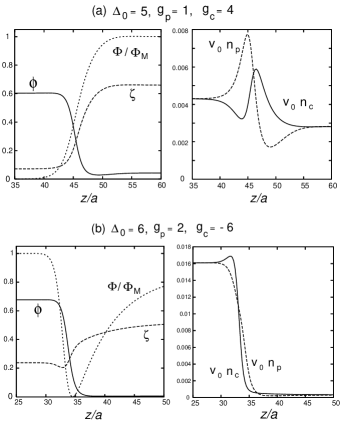
Figure 1: Interface profiles in the salt-free case for (a) $\Delta_{0}=5$, $g_{p}=1$, and $g_{c}=4$ (top) and for (b) $\Delta_{0}=8$, $g_{p}=2$, and $g_{c}=-6$ (bottom). Polymer volume fraction $\phi(z)$, normalized potential $\Phi(z)/\Phi_{M}$, and degree of ionization $\zeta(z)$ (left), and normalized charge densities $v_{0}n_{c}(z)$ and $v_{0}n_{p}(z)$ (right). The other parameters are common as $\chi=1$, $N=20$, $\nu_{M}=0.1$, $\varepsilon_{1}=-0.9\varepsilon_{0}$, and $\ell_{B}=8a/\pi$. Here $\Phi(z)$ is measured from its minimum, and $\Phi_{M}(=2.67T/e$ in (a) and $6.86T/e$ in (b)) is the difference of its maximum and minimum.

First we suppose coexistence of two salt-free phases, separated by a planar interface. Hereafter the quantities with the subscript $\alpha$ (the subscript $\beta$) denote the bulk values in the polymer-rich (solvent-rich) phase attained as $z\rightarrow-\infty$ (as $z\rightarrow\infty$). Namely, we write $n_{c\alpha}=n_{c}(-\infty)$ and $n_{c\beta}=n_{c}(\infty)$. Here we obtain $n_{c\alpha}$ or $n_{c\beta}$ from Eq.(2.29) and

$$\frac{n_{c\alpha}}{n_{c\beta}}=\frac{\phi_{\alpha}\zeta_{\alpha}}{\phi_{\beta}\zeta_{\beta}}=\exp({-g_{c}\Delta\phi-\Delta U})$$ (4.2)

from Eq.(2.17). Hereafter $\Delta\phi=\phi_{\alpha}-\phi_{\beta}$ is the composition difference and

$$\Delta U=e\Delta\Phi/T=e(\Phi_{\alpha}-\Phi_{\beta})/T$$ (4.3)

is the normalized Galvani potential difference. In terms of $Q_{\alpha}=4\nu_{M}\phi_{\alpha}/v_{0}K_{\alpha}$ and $Q_{\beta}=4\nu_{M}\phi_{\beta}/v_{0}K_{\beta}$, we obtain

$$\Delta U = g_{p}\Delta\phi+\ln\bigg{[}\frac{\sqrt{Q_{\beta}+1}-1}{\sqrt{Q_{\alpha}+1}-1}\bigg{]},$$ (4.4)

$$\frac{n_{c\beta}}{n_{c\alpha}} = \frac{\phi_{\beta}(\sqrt{Q_{\alpha}+1}+1)}{\phi_{\alpha}(\sqrt{Q_{\beta}+1}+1)}.$$ (4.5)

In particular, if $Q_{\alpha}\gg 1$ and $Q_{\beta}\gg 1$ (or $\zeta_{\alpha}\ll 1$ and $\zeta_{\beta}\ll 1$), we obtain $\Delta U\cong(g_{p}-g_{c})\Delta\phi/2+\ln(\phi_{\beta}/\phi_{\alpha})$ and ${n_{c\beta}/}{n_{c\alpha}}\cong\exp[(g_{p}+g_{c})\Delta\phi/2](\phi_{\beta}/\phi_{\alpha})^{1/2}$.

The interface profiles are extremely varied, sensitively depending on the molecular interaction parameters, $\Delta_{0}$, $g_{p}$, and $g_{c}$. As such examples, in Fig.1, we show salt-free interface profiles for (a) $\Delta_{0}=5$, $g_{p}=1$, and $g_{c}=4$ and (b) $\Delta_{0}=8$, $g_{p}=2$, and $g_{c}=-6$. In the $\alpha$ and $\beta$ regions, the degree of ionization $\zeta$ is $0.071$ and $0.65$ in (a) and is $0.24$ and $0.51$ in (b), respectively. The charge densities are multiplied by $v_{0}=a^{3}$. The $\Delta U=e(\Phi_{\alpha}-\Phi_{\beta})/T$ is $-2.67$ in (a) and $0.099$ in (b). Interestingly, in (b), $U(z)$ exhibits a deep minimum with $U_{\rm min}=U_{\beta}-5.98$ at the interface position. We can see appearance of the charge density $n_{c}-n_{p}$ around the interface, resulting in an electric double layer. The counterion density is shifted to the $\beta$ region in (a) because of positive $g_{c}$ and to the $\alpha$ region in (b) because of negative $g_{c}$. The parameter $\gamma_{p}$ in Eq.(3.11) is $0.75$ in (a) and $0.20$ in (b) in the $\alpha$ region, ensuring the stability of the $\alpha$ region. From Eq.(2.25) the surface tension $\gamma$ is calculated as $\gamma=0.0175T/a^{2}$ in (a) and as $0.0556T/a^{2}$ in (b), while we obtain $\gamma=0.050T/a^{2}$ without ions at the same $\chi=1$. In (a) the surface tension $\gamma$ is largely decreased because the electrostatic term in Eq.(2.25) is increased due to the formation of a large electric double layer. In (b), on the contrary, it is increased by $10\%$ due to depletion of the charged particles from the interface OnukiPRE .

IV.2 Interface with salt

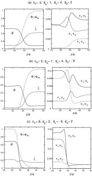
Figure 2: Interface profiles with mobile cations and anions for (a) $\Delta_{0}=5$, $g_{p}=1$, $g_{c}=4$, and $g_{2}=2$ (top), for (b) $\Delta_{0}=5$, $g_{p}=1$, $g_{c}=4$, and $g_{2}=-8$ (middle), and for (c) $\Delta_{0}=8$, $g_{p}=2$, $g_{c}=-6$, and $g_{2}=2$ (bottom). Curves represent $\phi(z)$, $\Phi(z)/\Phi_{M}$, and $\zeta(z)$ (left) and $v_{0}c_{c}(z)$, $v_{0}c_{p}(z)$, and $v_{0}c_{2}(z)$ (right) with $v_{0}n_{2\beta}=0.002$. Here $\Phi(z)$ is measured from its minimum, and $\Phi_{M}$ is the difference of its maximum and minimum. The other parameters are the same as those in Fig.1.

With addition of salt, interface profiles are even more complex. For simplicity, we consider a salt whose cations are of the same species as the counterions from the polymer. This is the example discussed at the end of Section 2. The free energy density in this case is still given by Eq.(2.7) if we set $n_{1}=0$ there. The densities of the mobile cations, the mobile anions, and the charged monomers are written as $n_{c}(z)$, $n_{2}(z)$, and $n_{p}(z)$, respectively. All the charged particles are monovalent. We treat $n_{2\beta}$ in the solvent-rich $\beta$ region as a control parameter, which is the salt density added in the $\beta$ region. The densities $n_{2}(z)$ and $n_{c}(z)$ depend on $z$ as

$$n_{2}(z) = n_{2\beta}\exp[g_{2}(\phi_{\beta}-\phi(z))-U_{\beta}+U(z)],$$

$$n_{c}(z) = n_{c\beta}\exp[g_{c}(\phi_{\beta}-\phi(z))+U_{\beta}-U(z)].$$ (4.6)

We write $S\equiv n_{2\beta}/K_{\beta}$ to avoid the cumbersome notation in the following. Use of the first line of Eq.(2.34) gives

$$n_{c\beta}=\frac{K_{\beta}}{2}\bigg{[}S-1+\sqrt{(S+1)^{2}+Q_{\beta}}\bigg{]}.$$ (4.7)

We use Eq.(2.33) in the $\alpha$ region to determine $n_{c\alpha}$. Since $n_{c\alpha}n_{2\alpha}/K_{\alpha}=n_{c\beta}n_{2\beta}/K_{\beta}$ from Eq.(4.5), $n_{c\alpha}$ obeys

$$(n_{c\alpha}-Sn_{c\beta}{K_{\alpha}}/{n_{c\alpha}})({1+n_{c\alpha}/K_{\alpha}})={v_{0}^{-1}\nu_{M}\phi_{\alpha}}.$$ (4.8)

In particular, if $n_{c\alpha}\gg K_{\alpha}$ or if $\zeta_{\alpha}\ll 1$, we find

$$n_{c\alpha}\cong K_{\alpha}^{1/2}(Sn_{c\beta}+v_{0}^{-1}\nu_{M}\phi_{\alpha})^{1/2},$$ (4.9)

$$\Delta U\cong g_{p}{\Delta\phi}+\frac{1}{2}\ln\bigg{[}\frac{n_{c\beta}^{2}/K_{\beta}^{2}}{Sn_{c\beta}/K_{\alpha}+Q_{\alpha}}\bigg{]}.$$ (4.10)

In Fig.2, we show profiles of $\phi(z)$, $\Phi(z)$, $\zeta(z)$, $n_{c}(z)$, $n_{2}(z)$, and $n_{p}(z)$ with $n_{2\beta}=0.002v_{0}^{-1}$ held fixed for three cases: (a) $\Delta_{0}=5$, $g_{p}=1$, $g_{c}=4$, and $g_{2}=2$; (b) $\Delta_{0}=5$, $g_{p}=1$, $g_{c}=4$, and $g_{2}=-8$; (c) $\Delta_{0}=8$, $g_{p}=2$, $g_{c}=-6$, and $g_{2}=2$. The normalized potential difference $\Delta U$ is $-1.61$ in (a), $-2.54$ in (b), and $1.88$ in (c), while the normalized surface tension $a^{2}\gamma/T$ is given by $0.0358$ in (a), $0.0233$ in (b), and $0.0554$ in (c). In (a) the cations and anions are both repelled from the interface into the $\beta$ region because of positive $g_{c}$ and $g_{2}$. In (b), owing to $g_{2}=-8$, the anions become richer in the $\alpha$ region than in the $\beta$ region, since they are strongly attracted to the polymer chains. There, despite $g_{c}=4$, the cations become also richer in the $\alpha$ region to satisfy the charge neutrality. In (c), we set $g_{c}=-6$, so the cations are strongly attracted to the polymer chains. The cations are also attracted into the $\alpha$ region. The electric dipole due to the double layer is reversed, yielding $\Delta U=U_{\alpha}-U_{\beta}>0$.

IV.3 Periodic state

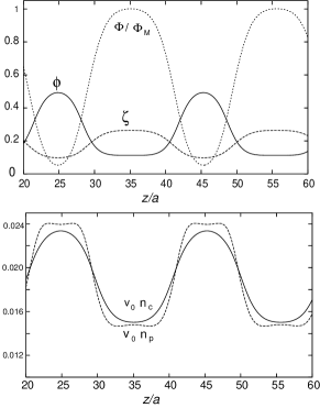
Figure 3: Periodic profiles in a salt-free mesophase with $\nu_{M}=0.5$, $\Delta_{0}=5$, $g_{p}=1$, and $g_{c}=4$. Top: $\phi(z)$. $\Phi(z)/\Phi_{M}$ with $\Phi_{M}=0.86T/e$, and $\zeta(z)$. Bottom: $v_{0}n_{c}(z)$ and $v_{0}n_{p}(z)$.

With varying the temperature (or $\chi$), the average composition $\langle{\phi}\rangle$, the amount of salt, there can emerge a number of mesophases sensitively depending on the various molecular parameters ($g_{i}$, $\Delta_{0}$, and $\nu_{M}$). In Fig.3, we show an example of a one-dimensional periodic state without salt. Here $\nu_{M}$ is set equal to $0.5$ and the charge densities are much increased. In this case, the degree of segregation and the charge heterogeneities are much milder than in the cases in Fig.1. Since the charge density $\rho(z)$ everywhere remains small, Eq.(2.31) locally holds approximately. Thus,

$$n_{c}(z)\cong\frac{\nu_{M}\phi(z)}{\sqrt{Q(z)+1/4}+1/2},$$ (4.11)

where $Q(z)$ is defined by Eq.(2.32) and $n_{p}(z)$ is determined by Eq.(2.26). The deviation of $n_{c}(z)$ from the right hand side of Eq.(4.10) gives $\Phi(z)$ as a first approximation. The above relation approximately holds slightly below the transition from a disordered state to a charge-density-wave state.

V Summary and remarks

The charge distributions in polyelectrolytes are extremely complex around interfaces and in mesoscopic states, sensitively depending on the molecular (solvation) interaction and the dissociation process. Our continuum theory takes account of these effects in the simplest manner, though it should be inaccurate on the angstrom scale.

Our main results are as follows. In Section 2, we have presented a continuum theory accounting for the solvation effect and the dissociation equilibrium. The degree of ionization is rather a dynamic variable dependent on the local electric potential. The surface tension in Eq.(2.25) consists of a positive gradient term and a negative electrostatic term, where the latter is significant as the electric double layer is enhanced as in the top panels in Figs.1 and 2. In Section 3, we have calculated the structure factor $S(q)$ of the composition fluctuations for polymer solutions with the solvation and ionization effects included. When the parameter $\gamma_{\rm p}$ in Eq.(3.11) or (3.12) exceeds unity in a one-phase state, a peak can appear at an intermediate wave number in $S(q)$. In such systems, a mesoscopic phase can emerge as the interaction parameter $\chi$ is increased. In Section 4, we have numerically solved the equilibrium equations in Section 2 to examine one-dimensional profiles of interfaces with and without salt and in a periodic state without salt. Though very preliminary and fragmentary, our numerical results demonstrate dramatic influence of the solvation interaction on inhomogeneous structures.

A number of complex effects should be further taken into account to properly describe polyelectrolytes. (i) Under Eq.(2.1) we have neglected the effect of the electrostatic interaction on the chain conformations to use the Flory-Huggins free energy density. Hence, as argued in the literature Barrat ; Rubinstein , our theory cannot be justified at small $\phi$. (ii) We have neglected the image interaction, which is known to increase the surface tension of a water-air interface at low ion densities Onsager . Generally, it arises from a deformation of the self-interaction of ions due to inhomogeneous $\varepsilon$ OnukiPRE . So it originates from the discrete nature of ions and is not accounted for in the free energy (2.7), where the electric field $\Phi$ is produced by the smoothly coarse-grained charge density $\rho$. (iii) At sufficiently low ion densities, we have neglected the ionic correlations giving rise to ion dipoles and clusters pair ; Krama and a free energy contribution due to the charge density fluctuations ($\propto\kappa^{3}$) Landau ; Onukibook . (iv) The phase diagram of mesophases including the solvation interaction remains unknown. To describe the mesophases we need to perform nonlinear analysis and computer simulations. (v) We have assumed a one-component water-like solvent. For two-component solvents we may predict a variety of effects. For example, with addition a small amount of water in a less polar solvent, hydration shells are formed around the hydrophilic ionized monomers and the counterions Is ; Osakai , leading to an increase of the degree of ionization. For not small water concentrations, we may well predict formation of complex mesoscopic structures mediated by the Coulombic and solvation interactions.

- (1) P.G. de Gennes, Scaling Concepts in Polymer Physics (Ithaca, Cornell Univ. Press) 1980.
- (2) J.L. Barrat and J.F. Joanny, Adv. Chem. Phys. XCIV, I. Prigogine, S.A. Rice Eds., John Wiley Sons, New York 1996.
- (3) A.V. Dobrynin and M. Rubinstein, Prog. Polym. Sci. 30, 1049 (2005).
- (4) E.Yu Kramarenko, A.R. Khoklov and K. Yoshikawa, Macromolecules 30, 3383 (1997).
- (5) E. Raphael and J. F. Joanny, Europhys. Lett. 13, 623 (1990).
- (6) I. Borukhov, D. Andelman, and H. Orland, Europhys. Lett.32, 499 (1995).
- (7) I. Borukhov, D. Andelman, R. Borrega, M. Cloitre, L. Leibler, and H. Orland, J. Phys. Chem. B 104, 11027 (2000).
- (8) J. N. Israelachvili, Intermolecular and Surface Forces (Academic Press, London, 1991).
- (9) V. Yu. Borye and I. Ya. Erukhimovich, Macromolecules 21, 3240 (1988).
- (10) J. F. Joanny and L. Leibler, J. Phys. (France) 51, 547 (1990).
- (11) D. E. Domidontova, I. Ya. Erukhimovich, and A. R. Khokhlov, Macromol. Theory Simul. 3, 661 (1994).
- (12) E. Yu. Kramarenko, I. Ya. Erukhimovich, and A. R. Khokhlov, Macromol. Theory Simul. 11, 462 (2002).
- (13) A. Onuki and H. Kitamura, J. Chem. Phys. 121, 3143 (2004).
- (14) A. Onuki, Phys. Rev. E 73, 021506 (2006); J. Chem. Phys. 128, 224704 (2008).
- (15) A. Onuki, EPL, 82, 58002 (2008).
- (16) A. Onuki, to be published in: ”Polymers, Liquids and Colloids in Electric Fields: Interfacial Instabilities, Orientation, and Phase-Transitions”, Eds. Y. Tsori and U. Steiner, World Scientific (2008).
- (17) K. Nishida, K. Kaji, and T. Kanaya, Macromolecules 28, 2472 (1995).
- (18) M. Shibayama, T. Tanaka, J. Chem. Phys. 102, 9392 (1995).
- (19) O. Braun, F. Boue, and F. Candau, Eur. Phys. J. E 7, 141 (2002).
- (20) K. Sadakane, H. Seto, H. Endo, and M. Shibayama, J. Phys. Soc. Jpn., 76, 113602 (2007).
- (21) I.F. Hakim and J. Lal, Europhys. Lett. 64, 204 (2003).
- (22) I.F. Hakim, J. Lal, and M. Bockstaller, Macromolecules 37, 8431 (2004).
- (23) Shi, A.-C.; Noolandi, J. Maromol. Theory Simul. 1999, 8(3), 214.
- (24) Q. Wang, T. Taniguchi, and G.H. Fredrickson, J. Phys. Chem B 2004, 108, 6733-6744; ibid. 2005, 109, 9855-9856.
- (25) L.D. Landau and E.M. Lifshitz, Statistical Physics (Pergamon, New York, 1964).
- (26) A. Onuki, Phase Transition Dynamics (Cambridge University Press, Cambridge, 2002).
- (27) L. Onsager and N. N. T. Samaras, J. Chem. Phys. 2, 528 (1934).
- (28) L. Degrve and F.M. Mazz, Molecular Phys. 101, 1443 (2003); A.A. Chen and R.V. Pappu, J. Phys. Chem. B 111, 6469 (2007).
- (29) P. Debye and K. Kleboth, J. Chem. Phys. 42, 3155 (1965).
- (30) Yu. Kramarenko, I. Ya. Erukhimovich, and A. R. Khokhlov, Macromol. Theory and Simul. 11, 462 (2002).
- (31) M. Born, Z. Phys. 1, 45 (1920).
- (32) Le Quoc Hung, J. Electroanal. Chem. 115, 159 (1980).
- (33) T. Osakai and K. Ebina, J. Phys. Chem. B 102, 5691 (1998).
- (34) K.V. Durme, H. Rahier, and B. van Mele, Macromolecules 38, 10155 (2005).
- (35) K. Sadakane, H. Seto, H. Endo, and M. Kojima, J. Appl. Crystallogr., 40, S527 (2007).
- (36) E.L. Eckfeldt and W.W. Lucasse, J. Phys. Chem. 47, 164 (1943).
- (37) B.J. Hales, G.L. Bertrand, and L.G. Hepler, J. Phys. Chem. 70, 3970 (1966).
- (38) V. Balevicius and H. Fuess, Phys. Chem. Chem. Phys. 1 ,1507 (1999).