Microscopic approach to high-temperature superconductors:
Pseudogap phase

Abstract

Despite the intense theoretical and experimental effort, an understanding of the superconducting pairing mechanism of the high-temperature superconductors leading to an unprecedented high transition temperature $T_{c}$ is still lacking. An additional puzzle is the unknown connection between the superconducting gap and the so-called pseudogap which is a central property of the most unusual normal state. Angle-resolved photoemission spectroscopy (ARPES) measurements have revealed a gap-like behavior on parts of the Fermi surface, leaving a non-gapped segment known as Fermi arc around the diagonal of the Brillouin zone. Two main interpretations of the origin of the pseudogap have been proposed: either the pseudogap is a precursor to superconductivity, or it arises from another order competing with superconductivity. Starting from the $t$-$J$ model, in this paper we present a microscopic approach to investigate physical properties of the pseudogap phase in the framework of a novel renormalization scheme called PRM. This approach is based on a stepwise elimination of high-energy transitions using unitary transformations. We arrive at a renormalized ’free’ Hamiltonian for correlated electrons. The ARPES spectral function along the Fermi surface turns out to be in good agreement with experiment: We find well-defined excitation peaks around $\omega=0$ near the nodal direction, which become strongly suppressed around the antinodal point. The origin of the pseudogap can be traced back to a suppression of spectral weight from incoherent excitations in a small $\omega$-range around the Fermi energy. Therefore, both mentioned interpretations of the origin of the pseudogap can not be held. Instead, the pseudogap is an inherent property of the unusual normal state caused by incoherent excitations. In a subsequent paper, also the supercunducting phase at moderate hole doping will be discussed within the PRM approachBS09 .

I Introduction

Since the discovery of superconductivity in the cuprates BM86 , enormous theoretical and experimental effort has been made to investigate the superconducting pairing mechanism which leads to an unprecedented high transition temperature $T_{c}$C99 -V97 . An additional puzzle is the unknown connection between the superconducting gap of the superconducting phase and the so-called pseudogap which is a central property of the most unusual normal state of the cuprates. In particular, the pseudogap has been subject to intense debates. Studies using angle resolved photoemssion spectroscopy (ARPES) have revealed several key features of the pseudogap in the cuprates by elucidating the detailed momentum and temperature dependenceN98 -CSG08 . It was found that the pseudogap opens on a part of the Fermi surface (FS) around the anti-nodal point, leaving a nongapped FS segment known as a Fermi arc around the nodal direction. The pseudogap also smoothly evolves with decreasing temperature into the SC gap and was, therefore, interpreted in favor of a “precursor pairing” scenario D96 ,L96 ,K08 . On the other hand, there are several experimental and theoretical reports which suggest a different origin for the pseudogap, such as caused by another order which competes with superconductivity S05 . Superconductivity is usually understood as an instability from a non-superconducting state. Therefore, often in theoretical investigations, the starting point was either the Fermi-liquid or the anti-ferromagnetic phase at large or low doping. In this paper, we take a different approach and only consider hole fillings, in which either a superconducting or a pseudogap phase is present.

A generally accepted model for the cuprates is the $t$-$J$ model which describes the electronic degrees of freedom in the copper-oxide planes for low energies. Alternatively, one could also start from a one-band Hubbard Hamiltonian as a minimal model. However, for low energy excitations, the latter model reduces to the $t$-$J$ model so that both models are equivalent. As our theoretical approach, we use a recently developed projector-based renormalization method which is called PRM PRM . The approach is based on a stepwise elimination of high-energy transitions using unitary transformations. We thus arrive at a renormalized ’free’ Hamiltonian for correlated electrons which can describe the pseudogap phase. The obtained ARPES spectral function along the Fermi surface is in good agreement with experiment: We find well-defined excitation peaks around $\omega=0$ near the nodal direction which are strongly suppressed around the antinodal point. The origin of the pseudogap can be traced back to a suppression of spectral weight of the incoherent excitations in a small $\omega$-range around the Fermi energy. Therefore, the usual interpretations of the pseudogap origin can not be held. Instead, the pseudogap is an inherent property of the unusual normal state caused by incoherent excitations.

First, after a short introduction of the model in Sec. II, it seems to be helpful, to start from a short outline of the basic ideas of our theoretical approach (PRM) in Sec. III. A review of this approach has been given elsewhere PRM . Then, in Sec. IV, the PRM will be applied to the $t$-$J$ model in order to investigate the pseudogap phase at moderate hole doping. The final results will be discussed in Sec. V. In a subsequent paper, the supercunducting phase will also be discussed.

II Model

A generally accepted model for the cuprates is the $t$-$J$ model. In particular, in the antiferromagnetic phase at small doping, it has turned out that it can be used to describe the electronic degrees of freedom at low energies. We adopt the same model also for somewhat larger hole concentrations, outside the antiferromagnetic phase, where the superconducting and the pseudogap phases appear

$${\cal H} = -\sum_{ij,\sigma}t_{ij}\,\hat{c}_{i\sigma}^{\dagger}\hat{c}_{j\sigma}-\mu\sum_{i\sigma}\hat{c}_{i\sigma}^{\dagger}\hat{c}_{i\sigma}+\sum_{ij}J_{ij}{\bf S}_{i}{\bf S}_{j}=:{\cal H}_{t}+{\cal H}_{J}.$$ (1)

The model consists of a hopping term ${\cal H}_{t}$ and an antiferromagnetic exchange ${\cal H}_{J}$. Here, $t_{ij}$ stands for the hopping matrix elements between nearest ($t$) and next-nearest ($t^{\prime}$) neighbors. $J_{ij}$ is the exchange coupling and $\mu$ is the chemical potential. The quantities

$$\hat{c}_{i\sigma}^{\dagger} = {c}_{i\sigma}^{\dagger}(1-n_{i,-\sigma}),\qquad\hat{c}_{i\sigma}={c}_{i\sigma}(1-n_{i,-\sigma})$$ (2)

are Hubbard creation and annihilation operators. They enter the model, since doubly occupancies of local sites are strictly forbidden due to the presence of strong electronic correlations. Note that the Hubbard operators restrict the unitary space to states with only either empty or singly occupied local sites. They obey nontrivial anti-commutation relations

$$[\hat{c}_{i\sigma}^{\dagger},\hat{c}_{j\sigma^{\prime}}]_{+} = \delta_{ij}\big{(}\delta_{\sigma\sigma^{\prime}}{\cal D}_{\sigma}(i)+\delta_{\sigma,-\sigma^{\prime}}S_{i}^{\sigma}\big{)},$$ (3)

where the operator

$${\cal D}_{\sigma}(i) = 1-n_{i,-\sigma}$$ (4)

can be interpreted as a projector which projects on the local subspace at site $i$ consisting of either an empty or a singly occupied state with spin $\sigma$. Finally, $n_{i\sigma}=c_{i\sigma}^{\dagger}c_{i\sigma}$ is the local occupation number operator for spin $\sigma$, and $S_{i}^{\sigma}$ is the $\sigma=\pm 1$ component of the local spin operator

$${\bf S}_{i} = \frac{1}{2}\sum_{\alpha\beta}\vec{\sigma}_{\alpha\beta}\hat{c}_{i\alpha}^{\dagger}\hat{c}_{i\beta},$$ (5)

where $\vec{\sigma}_{\alpha\beta}=\sum_{\nu}\sigma_{\alpha\beta}^{\nu}\,{\bf e}_{\nu}$ is the vector formed by the Pauli spin matrices. In Fourier notation, the $t$-$J$ model (1) reads

$${\cal H} = \sum_{{\bf k},\sigma}(\varepsilon_{\bf k}-\mu)\,\hat{c}_{{\bf k}\sigma}^{\dagger}\hat{c}_{{\bf k}\sigma}+\sum_{{\bf q}}J_{{\bf q}}{\bf S}_{\bf q}{\bf S}_{-{\bf q}}={\cal H}_{t}+{\cal H}_{J},$$ (6)

$$\varepsilon_{\bf k} = -\sum_{i(\neq j)}t_{ij}e^{i{\bf k}({\bf R}_{i}-{\bf R}_{j})},\qquad J_{\bf q}=\sum_{i(\neq j)}J_{ij}e^{i{\bf q}({\bf R}_{i}-{\bf R}_{j})}.$$

Note that for convenience, we shall somewhat change the notation. From now on, all energies will be measured from the chemical potential, i.e., $\varepsilon_{\bf k}-\mu$ will be denoted by $\varepsilon_{\bf k}$.

III Projector-based renormalization method (PRM)

Let us start with a short introduction to the projector-based renormalization method (PRM) BHS_2002 ; PRM which we shall use as our theoretical tool. The general idea is as follows: The method starts from a decomposition of a given many-particle Hamiltonian

$$\mathcal{H}=\mathcal{H}_{0}+\mathcal{H}_{1}$$ (7)

into an unperturbed part ${\cal H}_{0}$ and a perturbation ${\cal H}_{1}$. In $\mathcal{H}_{1}$, no parts should be contained which commute with $\mathcal{H}_{0}$. Therefore, $\mathcal{H}_{1}$ accounts for all transitions with non-zero energies between the eigenstates of $\mathcal{H}_{0}$. The aim of the PRM is to construct an effective Hamiltonian which has the same eigenspectrum as $\mathcal{H}$, and which can be solved. The first step is to construct a new renormalized Hamiltonian ${\cal H}_{\lambda}$ which depends on a given cutoff $\lambda$,

$$\mathcal{H}_{\lambda} = \mathcal{H}_{0,\lambda}+\mathcal{H}_{1,\lambda},$$ (8)

with renormalized parts ${\cal H}_{0,\lambda}$ and ${\cal H}_{1,\lambda}$. Thereby, ${\cal H}_{\lambda}$ should have the following properties: (i) The eigenvalue problem of $\mathcal{H}_{0,\lambda}$ can be solved

$$\mathcal{H}_{0,\lambda}|n^{\lambda}\rangle = E_{n}^{\lambda}|n^{\lambda}\rangle,$$

where $E_{n}^{\lambda}$ and $|n^{\lambda}\rangle$ are the renormalized eigenenergies and eigenvectors. (ii) From $\mathcal{H}_{1,\lambda}$, all transition operators are eliminated which have transition energies (with respect to $\mathcal{H}_{0,\lambda}$) larger than the cutoff energy $\lambda$. As shown in Refs. BHS_2002 ; PRM , the renormalization step from ${\cal H}$ to ${\cal H}_{\lambda}$ can be done by use of a unitary transformation. Therefore, the eigenspectrum of ${\cal H}_{\lambda}$ is the same as that of ${\cal H}$.

The realization of the renormalization starts from the construction of ${\cal H}_{\lambda}$. Here, the knowledge of the eigenvalue problem of ${\cal H}_{0,\lambda}$ is crucial. It can be used to define generalized projection operators, $\sf{P}_{\lambda}$ and $\sf{Q}_{\lambda}$,

$$\sf{P}_{\lambda}{\mathcal{A}} = \sum_{m,n}|n^{\lambda}\rangle\langle m^{\lambda}|\langle n^{\lambda}|\mathcal{A}|m^{\lambda}\rangle\,\Theta(\lambda-|E_{n}^{\lambda}-E_{m}^{\lambda}|),$$

$$\sf{Q}_{\lambda}\mathcal{A} = (\mathbf{1}-\sf{P}_{\lambda})\mathcal{A},$$ (9)

which act on usual operators ${\mathcal{A}}$ of the Hilbert space. Note that in Eq. (III) the vectors $|n^{\lambda}\rangle$ and $|m^{\lambda}\rangle$ are necessarily neither low- nor high energy eigenstates of $\mathcal{H}_{0,\lambda}$. $\sf{P}_{\lambda}$ projects on the part of ${\mathcal{A}}$ which consists of transition operators $|n^{\lambda}\rangle\langle m^{\lambda}|$ with excitation energies $|E_{n}^{\lambda}-E_{m}^{\lambda}|$ smaller than $\lambda$, whereas $\sf{Q}_{\lambda}$ projects on the high-energy transition operators of ${\mathcal{A}}$.

In terms of $\sf{P}_{\lambda}$ and $\sf{Q}_{\lambda}$, the property of ${\cal H}_{\lambda}$, not to allow transitions between eigenstates of ${\cal H}_{0,\lambda}$ with energy differences larger than $\lambda$, reads

$$\sf{Q}_{\lambda}\mathcal{H}_{\lambda}=0\quad\mbox{or}\quad\mathcal{H}_{\lambda} = \sf{P}_{\lambda}\mathcal{H}_{\lambda}\,.$$ (10)

The effective Hamiltonian ${\cal H}_{\lambda}$ is obtained from the original Hamiltonian ${\cal H}$ by use of a unitary transformation,

$$\mathcal{H}_{\lambda} = e^{X_{\lambda}}\;\mathcal{H}\;e^{-X_{\lambda}},$$ (11)

where $X_{\lambda}$ is the generator of the unitary transformation, and the condition (10) has to be fulfilled. The renormalization procedure starts from the cutoff energy $\lambda=\Lambda$ of the original model ${\cal H}$ and proceeds in steps of width $\Delta\lambda$ to lower values of $\lambda$. Every renormalization step is performed by means of a new unitary transformation,

$$\mathcal{H}_{(\lambda-\Delta\lambda)} = e^{X_{\lambda,\Delta\lambda}}\,\mathcal{H}_{\lambda}\,e^{-X_{\lambda,\Delta\lambda}}.$$ (12)

Here, the generator $X_{\lambda,\Delta\lambda}$ of the transformation from cutoff $\lambda$ to the reduced cutoff $(\lambda-\Delta\lambda)$ has to be chosen appropriately (see below). In this way, difference equations are derived which connect the parameters of ${\cal H}_{\lambda}$ with those of ${\cal H}_{(\lambda-\Delta\lambda)}$. They will be called renormalization equations. The limit $\lambda\rightarrow 0$ provides the desired effective Hamiltonian $\tilde{\cal H}={\cal H}_{\lambda\rightarrow 0}={\cal H}_{0,\lambda\rightarrow 0}$. The elimination of all transitions in the original perturbation $\mathcal{H}_{1}$ leads to renormalized parameters in ${\cal H}_{0,\lambda\rightarrow 0}$. Note that $\tilde{\cal H}$ is diagonal or at least quasi-diagonal and allows to evaluate all relevant physical quantities. The final expression for $\tilde{\cal H}$ depends on the parameter values of the original Hamiltonian $\mathcal{H}$. Note that $\tilde{\cal H}$ and ${\cal H}$ have, in principle, the same eigenspectrum because both Hamiltonians are connected by a unitary transformation.

What is left, is to find an appropriate expression for the generator $X_{\lambda,\Delta\lambda}$ of the unitary transformation which connects ${\cal H}_{\lambda}$ with ${\cal H}_{(\lambda-\Delta\lambda)}$. According to Eq. (10), $X_{\lambda,\Delta\lambda}$ is fixed by the condition ${\sf Q}_{\lambda-\Delta\lambda}{\cal H}_{\lambda-\Delta\lambda}=0$. As is shown in Refs. BHS_2002 ; PRM , one can find a perturbation expansion for $X_{\lambda,\Delta\lambda}$ in terms of ${\cal H}_{1}$. The lowest non-vanishing order reads

$$X_{\lambda,\Delta\lambda}^{(1)} = \frac{1}{\sf{L}_{0,\lambda}}\left[\sf{Q}_{(\lambda-\Delta\lambda)}\mathcal{H}_{1,\lambda}\right]+\cdots.$$ (13)

Here, ${\sf L}_{0,\lambda}$ is the Liouville operator, defined by the commutator ${\sf L}_{0,\lambda}{\cal A}=[{\cal H}_{0,\lambda},{\cal A}]$, for any operator quantity ${\cal A}$. Note that Eq. (13) can further be evaluated, in case the decomposition of ${\sf Q}_{(\lambda-\Delta\lambda)}{\cal H}_{1,\lambda}$ into eigenmodes of ${\sf L}_{0,\lambda}$ is known. Formally written, we decompose

$$\sf{Q}_{(\lambda-\Delta\lambda)}{\cal H}_{1,\lambda}=\sum_{\nu}{\bf F}^{\nu}_{\lambda,\Delta\lambda},\quad\mbox{where}\quad{\sf L}_{0,\lambda}\,{\bf F}^{\nu}_{\lambda,\Delta\lambda} = \omega^{\nu}_{\lambda,\Delta\lambda}\,{\bf F}^{\nu}_{\lambda,\Delta\lambda}\,,$$ (14)

so that $X^{(1)}_{\lambda,\Delta\lambda}$ is given by

$$X^{(1)}_{\lambda,\Delta\lambda} = \sum_{\nu}\frac{1}{\omega^{\nu}_{\lambda,\Delta\lambda}}{\bf F}^{\nu}_{\lambda,\Delta\lambda}.$$ (15)

IV Application to the $t$-$J$ model

IV.1 Renormalization ansatz

Our aim is to apply the PRM to the $t$-$J$ model which is a generally accepted model for the low-energy properties of the cuprate superconductors. We consider a regime with moderate hole-dopings. The hole concentrations should be large enough for the system to be outside the antiferromagnetic phase but small enough to be in the metallic phase. Our first aim is to find the decomposition of the Hamiltonian into an ’unperturbed’ part ${\cal H}_{0}$ and into a ’perturbation’ ${\cal H}_{1}$. We assume that the hopping element $t$ between nearest neighbors is large compared to the exchange coupling $J$. Therefore, ${\cal H}_{t}$ is the dominant part of the Hamiltonian in the metallic phase and should be included in ${\cal H}_{0}$. However, also ${\cal H}_{J}$ has a part, which commutes with the hopping term, and which will be called ${\cal H}_{J}^{(0)}$. Note that this part of ${\cal H}_{J}$ will not lead to transitions between the eigenstates of ${\cal H}_{t}$. Therefore, ${\cal H}_{t}$ and ${\cal H}_{J}^{(0)}$ together form the unperturbed Hamiltonian ${\cal H}_{0}$. The remaining part of ${\cal H}_{J}$ does not commute with ${\cal H}_{t}$ and forms the perturbation ${\cal H}_{1}$. Thus, we can write

$${\cal H}_{0} = {\cal H}_{t}+{\cal H}_{J}^{(0)},\qquad{\cal H}_{1}={\cal H}_{J}-{\cal H}_{J}^{(0)}.$$

In the framework of the PRM, the perturbation ${\cal H}_{1}$ will be integrated out by use of a unitary transformation. In lowest order perturbation theory, the generator of the unitary transformation $X_{\lambda,\Delta\lambda}$ is given by Eq. (15) and relies on the decomposition of ${\cal H}_{J}$ into the eigenmodes of ${\sf L}_{0}$. However, it will be impossible to find the exact decomposition of ${\cal H}_{J}$, due to the presence of Hubbard operators in ${\cal H}_{t}$. Therefore, we have to apply approximations. For this purpose, we start by decomposing the electronic spin operator

$${\bf S}_{\bf q} = \frac{1}{\sqrt{N}}\sum_{\alpha\beta}\frac{{\vec{\sigma}}_{\alpha\beta}}{2}\sum_{i}e^{i{\bf q}{\bf R}_{i}}\,\hat{c}_{i\alpha}^{\dagger}\hat{c}_{i\beta}$$ (16)

into eigenmodes of ${\sf L}_{t}$ instead of into eigenmodes of ${\sf L}_{0}$. Here, ${\sf L}_{t}$ is the Liouville operator corresponding to the hopping part ${\cal H}_{t}$ of ${\cal H}_{0}$. The exchange ${\cal H}_{J}$ is given by a sum over products of spin operators ${\bf S}_{\bf q}\cdot{\bf S}_{-{\bf q}}$. Therefore, the decomposition of ${\bf S}_{\bf q}$ into eigenmodes of ${\sf L}_{t}$ can be used to find an equivalent decomposition of ${\cal H}_{J}$.

The easiest way to decompose $\bf S_{q}$ is to derive an equation of motion for the time-dependent operator ${\bf S}_{\bf q}(t)$, where the time dependence is governed by ${\cal H}_{t}$,

$${\bf S}_{\bf q}(t)=e^{i{\cal H}_{t}t}\,{\bf S}_{\bf q}\,e^{-i{\cal H}_{t}t}=e^{i{\sf L}_{t}t}\,{\bf S}_{\bf q}.$$ (17)

Due to Eq. (3), the first time derivative reads

$$\frac{d}{dt}{\bf S}_{\bf q} = -\frac{i}{\sqrt{N}}\sum_{\alpha\beta}\frac{\vec{\sigma}_{\alpha\beta}}{2}\sum_{i\neq l}t_{il}\,e^{i{\bf q}{\bf R}_{i}}(\hat{c}_{l\alpha}^{\dagger}\hat{c}_{i\beta}-\hat{c}_{i\alpha}^{\dagger}\hat{c}_{l\beta})$$

$$= \frac{i}{\sqrt{N}}\sum_{\alpha\beta}\frac{\vec{\sigma}_{\alpha\beta}}{2}\sum_{i\neq l}t_{il}e^{i{\bf q}{\bf R}_{i}}(1-e^{i{\bf q}({\bf R}_{l}-{\bf R}_{i})})\,\hat{c}_{i\alpha}^{\dagger}\hat{c}_{l\beta}.$$

It can be interpreted as the hopping of a hole from some site $l$ to a neighboring site $i$ and vice versa. The second derivative is characterized by a twofold hopping,

$$\frac{d^{2}}{dt^{2}}{\bf S}_{\bf q} = -\frac{1}{\sqrt{N}}\sum_{i\neq l}t^{2}_{il}\,(e^{i{\bf q}{\bf R}_{l}}-e^{i{\bf q}{\bf R}_{i}})\,({\bf S}_{l}{\cal P}_{0}(i)-{\bf S}_{i}{\cal P}_{0}(l))$$

$$-\frac{1}{2\sqrt{N}}\sum_{\alpha\beta}\sum_{i\neq j}\sum_{j(\neq i\neq l)}\,t_{il}\,t_{lj}\,(e^{i{\bf qR}_{i}}-e^{i{\bf qR}_{l}})$$

$$\times\left\{\vec{\sigma}_{\alpha\beta}\left(\hat{c}_{j\alpha}^{\dagger}\,{\cal D}_{\alpha}(l)\,\hat{c}_{i\beta}+\hat{c}_{j,-\alpha}^{\dagger}S_{l}^{\alpha}\hat{c}_{i\beta}\right)+\vec{\sigma}_{\alpha\beta}^{*}\left(\hat{c}_{i\beta}^{\dagger}\,{\cal D}_{\alpha}(l)\,\hat{c}_{j\alpha}+c_{i\beta}^{\dagger}S_{l}^{-\alpha}\hat{c}_{m,-\alpha}\right)\right\}.$$

It has two different contributions. The first one describes the hopping of the hole from $i$ back to site $l$ from which it originally came and, equivalently, the hopping from $l$ back to $i$. The second term in Eq. (IV.1) stands for a twofold hopping away from the starting site.

Let us discuss the first contribution to Eq. (IV.1) in more detail. The operators

$${\cal P}_{0}(i)=(1-n_{i,\uparrow})(1-n_{i,\downarrow})$$ (20)

and ${\cal P}_{0}(l)$ can be interpreted as local projectors on the empty state at site $i$ and site $l$, respectively. They assure that the original sites $i$ and $l$ were empty before the first hop. Their presence results from the fact that doubly occupancies of local sites are strictly forbidden which is a consequence of the strong correlations in the $t$-$J$ model. In a further approximation, let us replace ${\cal P}_{0}(i)$ and ${\cal P}_{0}(l)$ by their expectation values,

$${\cal P}_{0}(i)\Rightarrow\langle(1-n_{i,\uparrow})(1-n_{i,\downarrow})\rangle_{0}=:P_{0},$$ (21)

which can be interpreted as the probability for a local site to be empty. Without the second term in Eq. (IV.1), we are led to the following equation of motion for ${\bf S}_{\bf q}(t)$:

$$\frac{d^{2}}{dt^{2}}{\bf S}_{\bf q} = -\hat{\omega}^{2}_{\bf q}\,{\bf S}_{\bf q}.$$ (22)

Obviously, the differential equation (22) describes an oscillatory motion of ${\bf S}_{\bf q}(t)$ with frequency $\omega_{\bf q}$, where

$$\hat{\omega}^{2}_{\bf q} = 2P_{0}(t^{2}_{{\bf q}=0}-t^{2}_{{\bf q}})=\hat{\omega}^{2}_{-{\bf q}}\geq 0,\quad\qquad t^{2}_{\bf q}=\sum_{l(\neq i)}t_{il}^{2}\,e^{i{\bf q}({\bf R}_{l}-{\bf R}_{i})}.$$ (23)

Note that the averaged projector $P_{0}=1-n$ also agrees with the hole concentration $\delta$ away from half-filling, i.e. $P_{0}=\delta=1-n$, where $n$ is the electron filling.

Before carrying on with the physical implications of Eqs. (22), (23), let us discuss the influence of the hole (or electron) hopping in Eq. (IV.1) to second nearest neighbors and also to more distant sites. As long as the dynamics of ${\bf S}_{\bf q}(t)$ is alone governed by the hopping Hamiltonian ${\cal H}_{t}$, all these hopping processes are important and would have to be taken into account. For instance, for a state close to half-filling outside the antiferromagnetic regime, a hole and a neighboring electron can freely interchange their positions for a system governed alone by ${\cal H}_{t}$. The hole can easily move through the lattice. However, the situation is different from the case, for which the dynamics is governed by ${\cal H}_{0}={\cal H}_{t}+{\cal H}_{J}^{(0)}$. Then, we have to decompose the perturbation ${\cal H}_{1}$ into eigenstates of ${\sf L}_{0}$, where ${\sf L}_{0}$ is the Liouville operator corresponding to ${\cal H}_{0}$. Thus, the dynamics of $\bf S_{q}$ is not governed alone by the hopping Hamiltonian ${\cal H}_{t}$ but also by the yet unknown commuting part ${\cal H}_{J}^{(0)}$ of ${\cal H}_{J}$. However, in Appendix A, it is shown that local antiferromagnetic spin fluctuations due to ${\cal H}_{J}^{(0)}$ restrict the hole motion to neighboring sites. The hopping to more distant sites is strongly suppressed by spin fluctuations. Therefore, the former equation of motion (22) for ${\bf S}_{\bf q}(t)$ turns out to be a good approximation for the case that the dynamics is determined by the full unperturbed Hamiltonian ${\cal H}_{0}$ including the exchange part.

The arguments in Appendix A are based on the evaluation of the dynamical spin susceptibility $\chi({\bf q},\omega)$ as follows. Using the Mori-Zwanzig projection formalism $\chi({\bf q},\omega)$ can be written as

$$\chi({\bf q},\omega) = \frac{-\omega_{\bf q}^{2}}{\omega^{2}-\omega_{\bf q}^{2}-\omega\,\Sigma_{\bf q}(\omega)}\,\chi_{\bf q}.$$ (24)

Here, $\omega_{\bf q}^{2}\approx\hat{\omega}_{\bf q}^{2}$ is approximately the frequency, given in Eq. (23), and $\Sigma_{\bf q}(\omega)$ is the selfenergy. The exact expression of $\Sigma_{\bf q}(\omega)$ in terms of the Mori scalar product reads

$$\Sigma_{\bf q}(\omega) = \frac{1}{(\dot{\bf S}_{\bf q}|\dot{\bf S}_{\bf q})}\,({\sf Q}\ddot{\bf S}_{\bf q}|\,\frac{1}{\omega-{\sf Q}{\sf L}_{0}{\sf Q}-i\eta}\,{\sf Q}\ddot{\bf S}_{\bf q}).\,$$ (25)

Here, ${\sf Q}$ is a generalized projection operator which projects perpendicular to ${\bf S}_{\bf q}$ and $\dot{\bf S}_{\bf q}$ (for details see Appendix D). Due to construction, the operator ${\sf Q}\ddot{\bf S}_{\bf q}$ in the ’bra’ and ’ket’ of Eq. (25) corresponds to the second line in Eq. (IV.1), and describes a twofold hopping away from the original site. Therefore, the selfenergy $\Sigma_{\bf q}(\omega)$ provides information about the hopping processes between next nearest neighbor sites and to more distant sites. In Appendix A the selfenergy $\Sigma_{\bf q}(\omega)$ is evaluated in a factorization approximation by including the spin fluctuations from ${\cal H}_{J}^{(0)}$. The result is shown in Fig. 1, where the imaginary part of $\Sigma_{\bf q}(\omega)$ for a small ${\bf q}$-vector is plotted (solid line) in the presence of spin fluctuations due to ${\cal H}_{J}^{(0)}$. As is seen, $\Sigma_{\bf q}(\omega)$ is rather small and almost $\omega$-independent over a wide frequency range. Thus, the only effect of $\Sigma_{\bf q}(\omega)$ is to give rise to a small damping and lineshift of the resonances of $\chi({\bf q},\omega)$. We have also repeated the same calculation for $\Im\Sigma_{\bf q}(\omega)$ in the absence of ${\cal H}_{J}^{(0)}$, i.e. when ${\cal H}_{0}$ is replaced by ${\cal H}_{t}$ (dashed line in Fig. 1). A strong $\omega$-dependence is found for small ${\bf q}$-values around $\omega=0$. This shows that long reaching hopping processes are important in this case. From these findings, one can conclude that the hopping to more distant than nearest neighbors is of minor importance as long as the exchange part ${\cal H}_{J}^{(0)}$ is not neglected in ${\cal H}_{0}$. A possible explanation would be that local antiferromagnetic correlations are still present at moderate hole doping outside the antiferromagnetic phase. They lead locally to strings of spin defects which are well known from the hole motion in the antiferromagnetic phase.

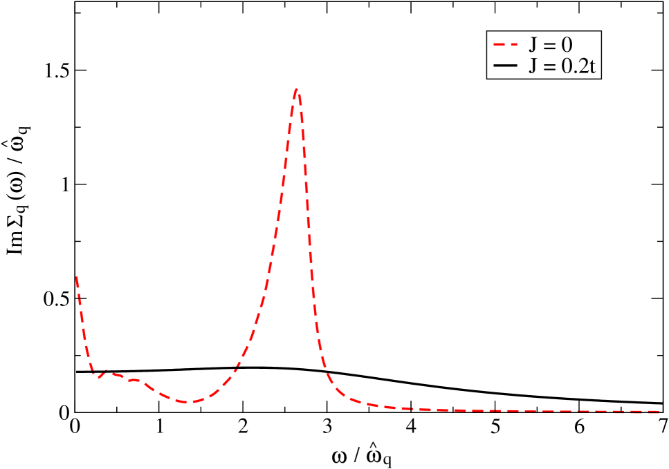
Figure 1: Imaginary part of the selfenergy $\Im\Sigma_{\bf q}(\omega)$ from Eq. (25) in the presence of spin fluctuations ($J=0.2t$, solid line) and in the absence of spin fluctuations ($J=0$, dashed line). The ${\bf q}$-vector is fixed to ${\bf q}=(\pi/20,\pi/20)$.

Let us come back to the discussion of the oscillation behavior in Eq. (IV.1) which can be understood as follows. When an electron hops to a neighboring site, it preferably hops back to the original site, since this was definitely empty after the first hop. In contrast, the hopping to next nearest neighbor sites is energetically unfavorable due to local antiferromagnetic order. As will be shown in a forthcoming paper BS09 , the proportionality of $\hat{\omega}^{2}_{\bf q}\sim\delta$ turns out to be the basic feature for the understanding of the superconducting pairing mechanism in the cuprates. The oscillation becomes less important for larger $\delta$ which agrees with the weakening of the superconducting phase for larger hole doping.

The solution of Eq. (22) is easily found,

$${\bf S}_{\bf q}(t) = {\bf S}_{\bf q}\,\cos{\hat{\omega}_{\bf q}t}+\frac{1}{\hat{\omega}_{\bf q}}\,\dot{\bf S}_{\bf q}\,\sin{\hat{\omega}_{\bf q}t}$$

$$= \frac{1}{2}({\bf S}_{\bf q}\,-\frac{i}{\hat{\omega}_{\bf q}}\,\dot{\bf S}_{\bf q})\,e^{i\hat{\omega}_{\bf q}\,t}+\frac{1}{2}({\bf S}_{\bf q}\,+\frac{i}{\hat{\omega}_{\bf q}}\,\dot{\bf S}_{\bf q})\,e^{-i\hat{\omega}_{\bf q}\,t},$$

where ${\bf S}_{\bf q}={\bf S}_{\bf q}(t=0)$ and $\dot{\bf S}_{\bf q}=\frac{d}{dt}{\bf S}_{\bf q}(t=0)$ was used. From Eq. (IV.1), the decomposition of ${\bf S}_{\bf q}$ into eigenmodes of ${\sf L}_{0}$ can immediately be identified,

$${\sf L}_{0}\,[\frac{1}{2}({\bf S}_{\bf q}\,\mp\frac{i}{\hat{\omega}_{\bf q}}\,\dot{\bf S}_{\bf q})] = \pm\omega_{\bf q}\,[\frac{1}{2}({\bf S}_{\bf q}\,\mp\frac{i}{\hat{\omega}_{\bf q}}\,\dot{\bf S}_{\bf q})],$$ (27)

which leads to the intended decomposition of the exchange ${\cal H}_{J}$ as follows:

$${\cal H}_{J} = \sum_{\bf q}J_{\bf q}\,{\bf S}_{\bf q}\,{\bf S}_{-{\bf q}}=\sum_{\bf q}J_{\bf q}\,\left({\cal A}_{0}({\bf q})+{\cal A}_{1}({\bf q})+{\cal A}_{1}^{\dagger}({\bf q})\right),$$ (28)

where

$${\cal A}_{0}({\bf q}) = \frac{1}{2}\left({\bf S}_{{\bf q}}{\bf S}_{-{\bf q}}+\frac{1}{\hat{\omega}_{\bf q}^{2}}\dot{\bf S}_{{\bf q}}\dot{\bf S}_{-{\bf q}}\right),$$ (29)

$${\cal A}_{1}({\bf q}) = \frac{1}{4}\left({\bf S}_{\bf q}-\frac{i}{\hat{\omega}_{\bf q}}\,\dot{\bf S}_{\bf q}\right)\,\left({\bf S}_{-{\bf q}}-\frac{i}{\hat{\omega}_{\bf q}}\,\dot{\bf S}_{-{\bf q}}\right),$$

$${\cal A}_{1}^{\dagger}({\bf q}) = \frac{1}{4}\left({\bf S}_{\bf q}+\frac{i}{\hat{\omega}_{\bf q}}\,\dot{\bf S}_{\bf q}\right)\,\left({\bf S}_{-{\bf q}}+\frac{i}{\hat{\omega}_{\bf q}}\,\dot{\bf S}_{-{\bf q}}\right),$$

and

$${\sf L}_{0}\,{\cal A}_{0}({\bf q}) = 0,\qquad{\sf L}_{0}\,{\cal A}_{1}({\bf q})=2\hat{\omega}_{\bf q}\,{\cal A}_{1}({\bf q}),\qquad{\sf L}_{0}\,{\cal A}_{1}^{\dagger}({\bf q})=-2\hat{\omega}_{\bf q}\,{\cal A}_{1}^{\dagger}({\bf q}).$$ (30)

Here, an additional approximation was used. In deriving Eqs. (30), the eigenmodes of the two spin operators ${\bf S_{q}}\cdot{\bf S}_{-{\bf q}}$ in the expression for ${\cal H}_{J}$ were taken separately from Eq. (27). In this way, all local configurations were disregarded, where two spin operators in local space are located on neighboring sites. Thereby, a possible hopping between the two sites would be obstructed. The inclusion of these processes would need additional considerations. However, they would not change our results substantially.

With Eqs. (29), we have arrived at the intended decomposition of the $t$-$J$ model. The Hamiltonian

$${\cal H} = \sum_{{\bf k}\sigma}\varepsilon_{\bf k}\hat{c}_{{\bf k}\sigma}^{\dagger}\hat{c}_{{\bf k}\sigma}+\sum_{\bf q}J_{\bf q}{\bf S}_{\bf q}{\bf S}_{-{\bf q}}$$ (31)

can be decomposed into an ’unperturbed’ part ${\cal H}_{0}$ and into a ’perturbation’ ${\cal H}_{1}$. It reads

$${\cal H}_{0} = {\cal H}_{t}+{\cal H}_{0,J}=:\sum_{{\bf k}\sigma}\varepsilon_{\bf k}\,\hat{c}_{{\bf k}\sigma}^{\dagger}\hat{c}_{{\bf k}\sigma}+\sum_{\bf q}J_{\bf q}\,{\cal A}_{0}({\bf q}),$$

$${\cal H}_{1} = \sum_{\bf q}J_{\bf q}\,\left({\cal A}_{1}({\bf q})+{\cal A}_{1}^{\dagger}({\bf q})\right).$$ (32)

The aim of the projector-based renormalization method (PRM) is to eliminate all transitions between the eigenstates of ${\cal H}_{0}$ which are induced by ${\cal H}_{1}$. Let us assume that all excitations with energies larger than a given cutoff $\lambda$ have already been eliminated. Then, the renormalized Hamiltonian ${\cal H}_{\lambda}$ should have the form

$${\cal H}_{\lambda} = \sum_{{\bf k}\sigma}\varepsilon_{{\bf k},\lambda}\,\hat{c}_{{\bf k}\sigma}^{\dagger}\hat{c}_{{\bf k}\sigma}+\sum_{\bf q}J_{{\bf q},\lambda}\,{\sf P}_{\lambda}{\bf S}_{\bf q}{\bf S}_{-{\bf q}}\,,$$ (33)

however, with $\lambda$-dependent prefactors $\varepsilon_{{\bf k},\lambda}$ and $J_{{\bf q},\lambda}$. Moreover, a projector ${\sf P}_{\lambda}$   was introduced which acts on operator variables. It guarantees that only transitions with excitation energies smaller than $\lambda$ remain from ${\bf S}_{\bf q}{\bf S}_{-{\bf q}}$.

The separation of ${\cal H}_{\lambda}$ into an unperturped part ${\cal H}_{0,\lambda}$ and a perturbation ${\cal H}_{1,\lambda}$ reads in analogy to Eq. (IV.1), ${\cal H}_{\lambda}={\cal H}_{0,\lambda}+{\cal H}_{1,\lambda}$, with

$${\cal H}_{0,\lambda} = {\cal H}_{t,\lambda}+\sum_{\bf q}J_{{\bf q},\lambda}\,{\cal A}_{0,\lambda}({\bf q})+E_{\lambda},$$

$${\cal H}_{1,\lambda} = \sum_{\bf q}J_{{\bf q},\lambda}\,\Theta(\lambda-|2\hat{\omega}_{{\bf q},\lambda}|)\left({\cal A}_{1,\lambda}({\bf q})+{\cal A}_{1,\lambda}^{\dagger}({\bf q})\right),$$ (34)

where we have used the $\lambda$-dependent extension of relation (30) in order to exploit the properties of ${\sf P}_{\lambda}$. Note that the $\Theta$-function $\Theta(\lambda-|2\hat{\omega}_{{\bf q},\lambda}|)$ in ${\cal H}_{1,\lambda}$ guarantees that only excitations with transition energies $|2\hat{\omega}_{{\bf q},\lambda}|$ smaller than $\lambda$ contribute to ${\cal H}_{1,\lambda}$. In Eq. (34), ${\cal H}_{t,\lambda}$ is the renormalized hopping term from Eq. (33), ${\cal H}_{t,\lambda}=\sum_{{\bf k}\sigma}\varepsilon_{{\bf k},\lambda}\,\hat{c}_{{\bf k}\sigma}^{\dagger}\hat{c}_{{\bf k}\sigma}$. Also, the parameters $J_{{\bf q},\lambda}$, $\hat{\omega}_{{\bf q},\lambda}$ and $E_{\lambda}$ in Eqs. (34) now depend on $\lambda$. Moreover, the new operators ${\cal A}_{\alpha,\lambda}({\bf q})$ ($\alpha=0,\pm 1$) depend on $\lambda$,

$${\cal A}_{0,\lambda}({\bf q}) = \frac{1}{2}\left({\bf S}_{{\bf q}}{\bf S}_{-{\bf q}}+\frac{1}{\hat{\omega}_{{\bf q},\lambda}^{2}}\dot{\bf S}_{{\bf q},\lambda}\dot{\bf S}_{-{\bf q},\lambda}\right),$$

$${\cal A}_{1,\lambda}({\bf q}) = \frac{1}{4}\left({\bf S}_{\bf q}-\frac{i}{\hat{\omega}_{{\bf q},\lambda}}\,\dot{\bf S}_{{\bf q},\lambda}\right)\,\left({\bf S}_{-{\bf q}}-\frac{i}{\hat{\omega}_{{\bf q},\lambda}}\,\dot{\bf S}_{-{\bf q},\lambda}\right),$$ (35)

$${\cal A}_{1,\lambda}^{\dagger}({\bf q}) = \frac{1}{4}\left({\bf S}_{\bf q}+\frac{i}{\hat{\omega}_{{\bf q},\lambda}}\,\dot{\bf S}_{{\bf q},\lambda}\right)\,\left({\bf S}_{-{\bf q}}+\frac{i}{\hat{\omega}_{{\bf q},\lambda}}\,\dot{\bf S}_{-{\bf q},\lambda}\right),$$

where $\hat{\omega}_{{\bf q},\lambda}$ and $\dot{\bf S}_{{\bf q},\lambda}$ are defined by

$$\hat{\omega}_{{\bf q},\lambda}^{2} = 2P_{0}\,(t^{2}_{{\bf q}=0,\lambda}-t^{2}_{{\bf q},\lambda}),\qquad t^{2}_{{\bf q},\lambda}=\sum_{i(\neq j)}t^{2}_{{ij},\lambda}\,e^{i{\bf q}({\bf R}_{i}-{\bf R}_{j})},$$

$$\dot{\bf S}_{{\bf q},\lambda} = \frac{i}{\hbar}[{\cal H}_{0,\lambda},{\bf S}_{{\bf q}}]\approx\frac{i}{\hbar}[{\cal H}_{t,\lambda},{\bf S}_{{\bf q}}].$$ (36)

IV.2 Generator of the unitary transformation

To derive renormalization equations for the parameters of ${\cal H}_{\lambda}$, we have to apply the unitary transformation (12) to ${\cal H}_{\lambda}$ in order to eliminate excitations within a new energy shell between $\lambda$ and $\lambda-\Delta\lambda$. We use the lowest order expression (15) for the new generator $X_{\lambda,\Delta\lambda}$,

$$X_{\lambda,\Delta\lambda} = \sum_{\bf q}\frac{J_{{\bf q},\lambda}}{2\hat{\omega}_{{\bf q},\lambda}}\Theta_{\bf q}(\lambda,\Delta\lambda)\left({\cal A}_{1,\lambda}({\bf q})-{\cal A}_{1,\lambda}^{\dagger}({\bf q})\right).$$ (37)

Here, $\Theta_{\bf q}(\lambda,\Delta\lambda)$ denotes a product of two $\Theta$-functions,

$$\Theta_{\bf q}(\lambda,\Delta\lambda) = \Theta(\lambda-|2\hat{\omega}_{{\bf q},\lambda}|)\,\Theta\left(|2\omega_{{\bf q},\lambda-\Delta\lambda}|-(\lambda-\Delta\lambda)\right),$$

which confines the elimination range to excitations with $|2\omega_{{\bf q},\lambda-\Delta\lambda}|$ larger than $\lambda-\Delta\lambda$ and $|2\hat{\omega}_{{\bf q},\lambda}|$ smaller than $\lambda$. Roughly speaking, for the case of a weak $\lambda$-dependence of $|\omega_{{\bf q},\lambda}|$, the elimination is restricted to all transitions within an energy shell between $\lambda-\Delta\lambda$ and $\lambda$. With (IV.1), the generator $X_{\lambda,\Delta\lambda}$ can also be expressed by

$$X_{\lambda,\Delta\lambda} = -i\sum_{\bf q}\frac{J_{{\bf q},\lambda}}{4\hat{\omega}_{{\bf q},\lambda}^{2}}\Theta_{\bf q}(\lambda,\Delta\lambda)\left({\bf S}_{\bf q}\,\dot{\bf S}_{-{\bf q},\lambda}+\dot{\bf S}_{{\bf q},\lambda}\,{\bf S}_{-{\bf q}}\right).$$ (38)

In the following, we restrict ourselves to the lowest order renormalization processes. Then, $J_{{\bf q},\lambda}$ will not be renormalized by higher orders in $J$, and we can use $J_{{\bf q},\lambda}=J_{\bf q}$ from the beginning.

IV.3 Renormalization equations

The unitary transformation (12), applied to the renormalization step between $\lambda$ and $\lambda-\Delta\lambda$, will be evaluated in perturbation theory in second order in $J_{\bf q}$,

$${\cal H}_{\lambda-\Delta\lambda} = e^{X_{\lambda,\Delta\lambda}}\,{\cal H}_{\lambda}\,e^{-X_{\lambda,\Delta\lambda}}={\cal H}_{\lambda-\Delta\lambda}^{(0)}+{\cal H}_{\lambda-\Delta\lambda}^{(1)}+{\cal H}_{\lambda-\Delta\lambda}^{(2)}+\cdots,$$ (39)

where

$${\cal H}_{\lambda-\Delta\lambda}^{(0)} = \sum_{{\bf k}\sigma}\varepsilon_{{\bf k},\lambda}\,\hat{c}_{{\bf k}\sigma}^{\dagger}\hat{c}_{{\bf k}\sigma}+E_{\lambda}={\cal H}_{t,\lambda}+E_{\lambda},$$

$${\cal H}_{\lambda-\Delta\lambda}^{(1)} = \sum_{\bf q}J_{{\bf q}}\,{\cal A}_{0,\lambda}({\bf q})+[X_{\lambda,\Delta\lambda},{\cal H}_{t,\lambda}]+\sum_{\bf q}J_{{\bf q}}\,\Theta(\lambda-|2\hat{\omega}_{{\bf q},\lambda}|)\left({\cal A}_{1,\lambda}({\bf q})+{\cal A}_{1,\lambda}^{\dagger}({\bf q})\right),$$

$${\cal H}_{\lambda-\Delta\lambda}^{(2)} = \frac{1}{2}[X_{\lambda,\Delta\lambda},[X_{\lambda,\Delta\lambda},{\cal H}_{t,\lambda}]\,]+\sum_{\bf q}J_{{\bf q}}\,[X_{\lambda,\Delta\lambda},{\cal A}_{0,\lambda}({\bf q})]$$ (40)

$$+\sum_{\bf q}J_{{\bf q}}\,\Theta(\lambda-|2\hat{\omega}_{{\bf q},\lambda}|)\,[\,X_{\lambda,\Delta\lambda},{\cal A}_{1,\lambda}({\bf q})+{\cal A}_{1,\lambda}^{\dagger}({\bf q})\,].$$

Let us first evaluate ${\cal H}_{\lambda-\Delta\lambda}^{(2)}$ from second order processes. The commutators in Eq. (IV.3) are explicitly evaluated in Appendix A. Then, we can compare the obtained result with the formal expression for ${\cal H}_{\lambda-\Delta\lambda}$ which has the same operator structure as ${\cal H}_{\lambda}$, with $\lambda$ is replaced by $\lambda-\Delta\lambda$. One obtains the following renormalization equation from the second order contributions in $J_{\bf q}$:

$$\varepsilon_{{\bf k},\lambda-\Delta\lambda}-\varepsilon_{{\bf k},\lambda} = \frac{1}{16N}\sum_{\bf q}\frac{J_{\bf q}^{2}}{\hat{\omega}_{{\bf q},\lambda}^{4}}\,\Theta_{\bf q}(\lambda,\Delta\lambda)\,(\varepsilon_{{\bf k}+{\bf q},\lambda}+\varepsilon_{{\bf k}-{\bf q},\lambda}-2\varepsilon_{{\bf k},\lambda})\,\langle\dot{\bf S}_{{\bf q},\lambda}\,\dot{\bf S}_{-{\bf q},\lambda}\rangle$$

$$+\frac{3}{2N}\sum_{{\bf q}\sigma}\left(\frac{J_{\bf q}}{4\hat{\omega}_{\bf q}^{2}}\right)^{2}\,\Theta_{\bf q}(\lambda,\Delta\lambda)\,(\varepsilon_{{\bf k},\lambda}-\varepsilon_{{\bf k}-{\bf q},\lambda})^{2}$$

$$\times\left[\frac{1}{N}\sum_{{\bf k}^{\prime}\sigma^{\prime}}(2\varepsilon_{{\bf k}^{\prime},\lambda}-\varepsilon_{{\bf k}^{\prime}+{\bf q},\lambda}-\varepsilon_{{\bf k}^{\prime}-{\bf q},\lambda})\langle\hat{c}_{{\bf k}^{\prime}\sigma^{\prime}}^{\dagger}\hat{c}_{{\bf k}^{\prime}\sigma^{\prime}}\rangle\right]\,n_{{\bf k}-{\bf q}\alpha}^{(NL)},$$

where we have defined

$$n_{{\bf k},\sigma}^{(NL)} = \langle\hat{c}_{{\bf k}\sigma}^{\dagger}\hat{c}_{{\bf k}\sigma}\rangle-\frac{1}{N}\sum_{{\bf k}^{\prime}}\langle\hat{c}_{{\bf k}^{\prime}\sigma}^{\dagger}\hat{c}_{{\bf k}^{\prime}\sigma}\rangle$$ (42)

as non-local part of the one-particle occupation number per spin direction. An equivalent equation also exists for $E_{\lambda-\Delta\lambda}$. Note that in Eq. (IV.3) an additional factorization approximation was used in order to extract all terms which have the same operator structure as ${\cal H}_{\lambda}$. The quantity $\langle\dot{\bf S}_{{\bf q},\lambda}\dot{\bf S}_{-{\bf q},\lambda}\rangle$ is a correlation function of the time derivatives of ${\bf S}_{\bf q}$ which can easily be evaluated from Eq. (101). Note that an additional contribution to $\varepsilon_{{\bf k},\lambda-\Delta\lambda}$, proportional to the correlation function $\langle{\bf S}_{\bf q}\cdot{\bf S}_{-{\bf q}}\rangle$, has been neglected. The remaining expectation values in Eq. (IV.3) have to be calculated separately. In principle, they should be defined with the $\lambda$-dependent Hamiltonian ${\cal H}_{\lambda}$, because the factorization approximation was employed for the renormalization step from ${\cal H}_{\lambda}$ to ${\cal H}_{\lambda-\Delta\lambda}$. However, ${\cal H}_{\lambda}$ still contains interactions which prevent a straight evaluation of $\lambda$-dependent expectation values. The best way to circumvent this difficulty is to calculate the expectation values with the full Hamiltonian ${\cal H}$ instead of with ${\cal H}_{\lambda}$. In this case, the renormalization equations can be solved self-consistently, as will be discussed below.

Note that the renormalization (IV.3) of $\varepsilon_{{\bf k},\lambda}$ was evaluated from the second order part ${\cal H}_{\lambda-\Delta\lambda}^{(2)}$ of the Hamiltonian (IV.3). Thus, we are led to

$${\cal H}_{\lambda-\Delta\lambda} = {\cal H}_{t,\lambda-\Delta\lambda}+{\cal H}_{\lambda-\Delta\lambda}^{(1)}+E_{\lambda-\Delta\lambda},$$ (43)

where ${\cal H}_{t,\lambda-\Delta\lambda}=\sum_{{\bf k},\sigma}\varepsilon_{{\bf k},\lambda-\Delta\lambda}\,\hat{c}_{{\bf k}\sigma}^{\dagger}\hat{c}_{{\bf k}\sigma}$. What remains is to evaluate the renormalization part ${\cal H}_{\lambda-\Delta\lambda}^{(1)}$ in first order in $J_{\bf q}$ to ${\cal H}_{\lambda-\Delta\lambda}$. First, the second term on the right hand side of Eq. (IV.3) can be rewritten, since

$$[X_{\lambda,\Delta\lambda},{\cal H}_{t,\lambda}] = -\sum_{\bf q}J_{{\bf q}}\Theta_{\bf q}(\lambda,\Delta\lambda)\,\left({\cal A}_{1,\lambda}({\bf q})+{\cal A}_{1,\lambda}^{\dagger}({\bf q})\right).$$

Then, by combining the second and third term, we find

$${\cal H}_{\lambda-\Delta\lambda}^{(1)} = \sum_{\bf q}J_{{\bf q}}\,{\cal A}_{0,\lambda}({\bf q})$$

$$+ \sum_{\bf q}J_{{\bf q}}\,\Theta(\lambda-|2\hat{\omega}_{{\bf q},\lambda}|)\,\Theta(\lambda-\Delta\lambda-|2\hat{\omega}_{{\bf q},\lambda-\Delta\lambda}|)\left({\cal A}_{1,\lambda}({\bf q})+{\cal A}_{1,\lambda}^{\dagger}({\bf q})\right).$$

The excitation energies of ${\cal A}_{1,\lambda}({\bf q})$ and ${\cal A}_{1,\lambda}^{\dagger}({\bf q})$ are restricted to $|2\hat{\omega}_{{\bf q},\lambda}|\leq\lambda$ by the first $\Theta$-function in Eq. (IV.3). This condition is automatically fulfilled by the second $\Theta$-function, in the case that $|2\hat{\omega}_{{\bf q},\lambda-\Delta\lambda}|$ only weakly depends on $\lambda$ and we can replace $\lambda$ by $\lambda-\Delta\lambda$. By introducing the projector ${\sf P}_{\lambda-\Delta\lambda}$ on all low-energy transition operators with energies smaller than $\lambda-\Delta\lambda$, we find

$${\cal H}_{\lambda-\Delta\lambda}^{(1)} = \sum_{\bf q}J_{{\bf q}}\,{\sf P}_{\lambda-\Delta\lambda}\left({\cal A}_{0,\lambda}({\bf q})+{\cal A}_{1,\lambda}({\bf q})+{\cal A}_{1,\lambda}^{\dagger}({\bf q})\right)$$ (45)

$$= \sum_{\bf q}J_{\bf q}{\sf P}_{\lambda-\Delta\lambda}\,{\bf S}_{\bf q}\cdot{\bf S}_{-{\bf q}},$$

where we have used the representation (28) for the scalar product ${\bf S}_{\bf q}\cdot{\bf S}_{-{\bf q}}$,

$${\bf S}_{\bf q}\cdot{\bf S}_{-{\bf q}} = {\cal A}_{0,\lambda}({\bf q})+{\cal A}_{1,\lambda}({\bf q})+{\cal A}_{1,\lambda}^{\dagger}({\bf q}).$$ (46)

Finally, for the total Hamiltonian ${\cal H}_{\lambda-\Delta\lambda}$, we obtain according to (43)

$${\cal H}_{\lambda-\Delta\lambda} = \sum_{{\bf k},\sigma}\varepsilon_{{\bf k},\lambda-\Delta\lambda}\,\hat{c}_{{\bf k}\sigma}^{\dagger}\hat{c}_{{\bf k}\sigma}+\sum_{\bf q}J_{\bf q}{\sf P}_{\lambda-\Delta\lambda}\,{\bf S}_{\bf q}\cdot{\bf S}_{-{\bf q}}+E_{\lambda-\Delta\lambda}.$$ (47)

Note that this expression completely agrees with the Hamiltonian at cutoff $\lambda$, when $\lambda$ is replaced by $\lambda-\Delta\lambda$. The required decomposition into ${\cal H}_{0,\lambda-\Delta\lambda}$ and ${\cal H}_{1,\lambda-\Delta\lambda}$ is found as follows. We use again the relation (46), with $\lambda$ is replaced by $\lambda-\Delta\lambda$, and rewrite ${\cal H}_{\lambda-\Delta\lambda}^{(1)}$ as

$${\cal H}_{\lambda-\Delta\lambda}^{(1)} = \sum_{\bf q}J_{{\bf q}}\,{\sf P}_{\lambda-\Delta\lambda}\left({\cal A}_{0,\lambda-\Delta\lambda}({\bf q})+{\cal A}_{1,\lambda-\Delta\lambda}({\bf q})+{\cal A}_{1,\lambda-\Delta\lambda}^{\dagger}({\bf q})\right).$$ (48)

Using again Eq. (45), we arrive at the renormalized Hamiltonian ${\cal H}_{\lambda-\Delta\lambda}={\cal H}_{0,\lambda-\Delta\lambda}+{\cal H}_{1,\lambda-\Delta\lambda}$ in the following form,

$${\cal H}_{0,\lambda-\Delta\lambda} = {\cal H}_{t,\lambda-\Delta\lambda}+\sum_{\bf q}J_{{\bf q}}\,{\cal A}_{0,\lambda-\Delta\lambda}({\bf q})+E_{\lambda-\Delta\lambda},$$

$${\cal H}_{1,\lambda-\Delta\lambda} = \sum_{\bf q}J_{{\bf q}}\,\Theta(\lambda-\Delta\lambda-|\hat{\omega}_{{\bf q},\lambda-\Delta\lambda}|)\,\left({\cal A}_{1,\lambda-\Delta\lambda}({\bf q})+{\cal A}_{1,\lambda-\Delta\lambda}^{\dagger}({\bf q})\right).$$ (49)

As expected, the renormalized Hamiltonians ${\cal H}_{0,\lambda-\Delta\lambda}$ and ${\cal H}_{1,\lambda-\Delta\lambda}$ have the same operator structure as at cutoff $\lambda$. Therefore, we can formulate a renormalization scheme as follows: We start from the original $t$-$J$ model, where the energy cutoff is denoted by ${\lambda=\Lambda}$. Starting from a guess for the unknown expectation values, which enter the renormalization equation (IV.3), we proceed by eliminating all excitations in steps $\Delta\lambda$ from $\lambda=\Lambda$ down to $\lambda=0$. Thereby, the parameters of the Hamiltonian change in steps according to the renormalization equation (IV.3). In this way, we obtain the following model at $\lambda=0$:

$${\cal H}_{\lambda=0} = {\cal H}_{t,\lambda=0}+\sum_{\bf q}J_{\bf q}{\sf P}_{\lambda=0}{\bf S}_{\bf q}\cdot{\bf S}_{-{\bf q}}+E_{\lambda=0}$$

$$= \sum_{{\bf k}\sigma}\varepsilon_{{\bf k},\lambda=0}\,\hat{c}_{{\bf k}\sigma}^{\dagger}\,\hat{c}_{{\bf k}\sigma}+\sum_{\bf q}J_{{\bf q}}\,{\cal A}_{{0},\lambda=0}({\bf q})+E_{\lambda=0}.$$

Note that in Eq. (IV.3) the perturbation ${\cal H}_{1}$ is completely integrated out. Only the part of the exchange, which commutes with the hopping term, remains.

Unfortunately, due to the presence of the ${\cal A}_{0}$-term, the Hamiltonian ${\cal H}_{\lambda=0}$ can not be diagonalized. It does not yet allow us to recalculate the expectation values. Therefore, a further approximation is necessary which consists of a factorization of the second term

$$\sum_{\bf q}J_{{\bf q}}\,{\cal A}_{{0},\lambda=0}({\bf q}) = \sum_{\bf q}\frac{J_{\bf q}}{2}\left({\bf S}_{{\bf q}}{\bf S}_{-{\bf q}}+\frac{1}{\hat{\omega}_{{\bf q},\lambda=0}^{2}}\dot{\bf S}_{{\bf q},\lambda=0}\dot{\bf S}_{-{\bf q},\lambda=0}\right).$$ (51)

According to Appendix B, ${\cal H}_{\lambda=0}$ can finally be replaced by a modified Hamiltonian which will be denoted by $\tilde{\cal H}^{(1)}$,

$$\tilde{\cal H}^{(1)} = \sum_{{\bf k}\sigma}\tilde{\varepsilon}_{\bf k}^{(1)}\,\hat{c}_{{\bf k}\sigma}^{\dagger}\,\hat{c}_{{\bf k}\sigma}+\sum_{\bf q}\frac{J_{{\bf q}}}{2}\,{\bf S}_{\bf q}\,{\bf S}_{-{\bf q}}+\tilde{E}^{(1)},$$ (52)

where the electron energy is modified according to

$$\tilde{\varepsilon}_{\bf k}^{(1)} = \varepsilon_{{\bf k},\lambda=0}-\frac{1}{N}\sum_{\bf q}\frac{3J_{\bf q}}{4\hat{\omega}^{2}_{{\bf q},\lambda=0}}(\varepsilon_{{\bf k},\lambda=0}-\varepsilon_{{\bf k}-{\bf q},\lambda=0})^{2}\,n_{{\bf k}-{\bf q},\sigma}^{(NL)},$$ (53)

and $n_{{\bf k},\sigma}^{(NL)}$ is defined in Eq. (42). Note that the operator structure of $\tilde{\cal H}^{(1)}$ agrees with that of the original $t$-$J$ model of Eq. (31). However, the parameters have changed. Most important, the strength of the exchange coupling in Eq. (52) is decreased by a factor $1/2$. This property allows us to start the whole renormalization procedure again. We consider the modified $t$-$J$ model of Eq. (52) as our new initial Hamiltonian, which has to be renormalized again. The initial values of $\tilde{\cal H}^{(1)}$ at cutoff $\lambda=\Lambda$ are $\tilde{\varepsilon}_{\bf k}^{(1)}$ and $J_{\bf q}/2$. After the new renormalization cycle the exchange coupling of the new renormalized Hamiltonian $\tilde{\cal H}^{(2)}$ is again decreased by a factor $1/2$, till after a sufficiently large number of renormalization cycles ($n\rightarrow\infty$) the exchange operator completely disappears. Thus, we finally arrive at a ’free’ model

$$\tilde{\cal H} = \sum_{{\bf k}\sigma}\tilde{\varepsilon}_{\bf k}\,\hat{c}_{{\bf k}\sigma}^{\dagger}\,\hat{c}_{{\bf k}\sigma}+\tilde{E}\,,$$ (54)

where we have introduced as new notations $\tilde{\cal H}=\tilde{\cal H}^{(n\rightarrow\infty)}$, $\tilde{\varepsilon}_{\bf k}=\tilde{\varepsilon}_{\bf k}^{(n\rightarrow\infty)}$, and $\tilde{E}=\tilde{E}^{(n\rightarrow\infty)}$. Note that the Hamiltonian $\tilde{\cal H}$ now allows us to recalculate the unknown expectation values. With the new values, the whole renormalization procedure can be started again till, after a sufficiently large number of such overall cycles, the expectation values have converged. The renormalization equations are solved self-consistently. However, note that the fully renormalized Hamiltonian (54) is actually not a ’free’ model. Instead, it is still subject to strong electronic correlations which are built in by the presence of the Hubbard operators. Therefore, to evaluate the expectation values, further approximations have to be made.

IV.4 Evaluation of expectation values

The expectation values in Eqs. (IV.3) and (53) are formed with the full Hamiltonian. To evaluate expectation values for operator variables ${\cal A}$, we have to apply the unitary transformation also on ${\cal A}$,

$$\langle{\cal A}\rangle = \frac{\mbox{Tr}\,({\cal A}\,e^{-\beta{\cal H}})}{\mbox{Tr}\,e^{-\beta{\cal H}}}=\langle{\cal A}(\lambda)\rangle_{{\cal H}_{\lambda}}=\langle\tilde{\cal A}\rangle_{\tilde{\cal H}}\,,$$ (55)

where we have defined ${\cal A}(\lambda)=e^{X_{\lambda}}\;{\cal A}e^{-X_{\lambda}}$ and ${\tilde{\cal A}}={\cal A}(\lambda\rightarrow 0)$. Thus, additional renormalization equations for ${\cal A}(\lambda)$ have to be derived.

As an example, let us consider the angle-resolved photoemission (ARPES) spectral function. It is defined by

$${A}({\bf k},\omega) = \frac{1}{2\pi}\int_{-\infty}^{\infty}\big{<}\hat{c}_{{\bf k}\sigma}^{\dagger}(-t)\;\hat{c}_{{\bf k}\sigma}\big{>}\;e^{i\omega t}dt=\big{<}\hat{c}_{{\bf k}\sigma}^{\dagger}\,\delta({\sf L}+\omega)\;\hat{c}_{{\bf k}\sigma}\big{>}$$ (56)

and can be rewritten by use of the dissipation-fluctuation theorem as

$${A}({\bf k},\omega) = \frac{1}{1+e^{\beta\omega}}\Im G({\bf k},\omega)\,,$$ (57)

where $\Im G({\bf k},\omega)$ is the dissipative part of the anti-commutator Green function

$$\Im G({\bf k},\omega) = \frac{1}{2\pi}\,\int_{-\infty}^{\infty}\big{<}[\hat{c}_{{\bf k}\sigma}^{\dagger}(-t)\,,\;\hat{c}_{{\bf k}\sigma}]_{+}\big{>}\;e^{i\omega t}dt=\big{<}[\hat{c}_{{\bf k}\sigma}^{\dagger}\,,\,\delta({\sf L}+\omega)\;\hat{c}_{{\bf k}\sigma}]_{+}\big{>}.$$

The time dependence and the expectation value are formed with the full Hamiltonian ${\cal H}$, and $\sf L$ is the Liouville operator corresponding to ${\cal H}$. According to Eq. (55), the anti-commutator Green function can be expressed by

$${\Im G}({\bf k},\omega) = \big{<}[\hat{c}_{{\bf k}\sigma}^{\dagger}(\lambda)\,,\,\delta({\sf L}_{\lambda}+\omega)\;\hat{c}_{{\bf k}\sigma}(\lambda)]_{+}\big{>}_{\lambda}\,,$$ (58)

where now the creation and annihilation operators are also subject to the unitary transformation. To evaluate $A({\bf k},\omega)$, we have to derive renormalization equations for $\hat{c}_{{\bf k}\sigma}(\lambda)$ and $\hat{c}_{{\bf k}\sigma}^{\dagger}(\lambda)$. According to Appendix C, the following ansatz for $\hat{c}_{{\bf k}\sigma}(\lambda)$ can be used:

$$\hat{c}_{{\bf k}\sigma}(\lambda) = u_{{\bf k},\lambda}\hat{c}_{{\bf k}\sigma}+\frac{1}{2N}\sum_{{\bf qk}^{\prime}}v_{{\bf k},{\bf q},\lambda}\,\frac{J_{\bf q}}{4\hat{\omega}^{2}_{{\bf q},\lambda}}\,\sum_{\alpha\beta\gamma}(\vec{\sigma}_{\alpha\beta}\cdot\vec{\sigma}_{\sigma\gamma})(\varepsilon_{{\bf k}^{\prime},\lambda}-\varepsilon_{{\bf k}^{\prime}+{\bf q},\lambda})\,\,\hat{c}^{\dagger}_{{\bf k}^{\prime}+{\bf q}\alpha}\ \hat{c}_{{\bf k}^{\prime}\beta}\ \hat{c}_{{\bf k}+{\bf q}\gamma}.$$

It can be justified from lowest order perturbation theory. Note that the $\lambda$-dependence is transferred to the parameters $u_{{\bf k},\lambda}$ and $v_{{\bf k},{\bf q},\lambda}$. Also the quantities $\hat{\omega}_{{\bf q},\lambda}$ and $\varepsilon_{{\bf k},\lambda}$ depend on $\lambda$. However, having in mind perturbation theory in $J$, this $\lambda$-dependence will be neglected in the numerical evaluation of Sec. V below. According to Appendix C, the renormalization equations for $u_{{\bf k},\lambda}$ and $v_{{\bf k},{\bf q},\lambda}$ read

$$u_{{\bf k},\lambda-\Delta\lambda}^{2} = u_{{\bf k},\lambda}^{2}-\frac{3}{2N^{2}}\sum_{{\bf q}{\bf k}^{\prime}}\left(\frac{J_{\bf q}}{4\hat{\omega}_{\bf q}^{2}}\right)^{2}\Theta_{\bf q}(\lambda,\Delta\lambda)(\varepsilon_{{\bf k}^{\prime},\lambda}-\varepsilon_{{\bf k}^{\prime}+{\bf q},\lambda})^{2}\left\{\left(\frac{u_{{\bf k},\lambda}}{2}\right)^{2}+u_{{\bf k},\lambda}\,v_{{\bf k},{\bf q},\lambda}\right\}$$ (60)

$$\times\left\{n_{{\bf k}^{\prime}+{\bf q}}m_{{\bf k}^{\prime}}+n_{{\bf k}+{\bf q}}(D+n_{{\bf k}^{\prime}}-n_{{\bf k}^{\prime}+{\bf q}})\right\}$$

$$+ \frac{3}{4N^{2}}\sum_{{\bf q}{\bf q}^{\prime}}\frac{J_{\bf q}}{4\hat{\omega}_{\bf q}^{2}}\,\frac{J_{{\bf q}^{\prime}}}{4\hat{\omega}_{{\bf q}^{\prime}}^{2}}(\varepsilon_{{\bf k}+{\bf q}^{\prime},\lambda}-\varepsilon_{{\bf k}+{\bf q}+{\bf q}^{\prime},\lambda})\,(\varepsilon_{{\bf k}+{\bf q},\lambda}-\varepsilon_{{\bf k}+{\bf q}+{\bf q}^{\prime},\lambda})$$

$$\times\left\{v_{{\bf k},{\bf q}^{\prime},\lambda}\Theta_{\bf q}(\lambda,\Delta\lambda)+v_{{\bf k},{\bf q},\lambda}\Theta_{{\bf q}^{\prime}}(\lambda,\Delta\lambda)\right\}\frac{u_{{\bf k},\lambda}}{2}$$

$$\times\left\{n_{{\bf k}+{\bf q}^{\prime}}(n_{{\bf k}+{\bf q}+{\bf q}^{\prime}}-n_{{\bf k}+{\bf q}}-D)-m_{{\bf k}+{\bf q}}n_{{\bf k}+{\bf q}+{\bf q}^{\prime}}\right\}$$

and

$$v_{{\bf k},{\bf q},\lambda-\Delta\lambda} = v_{{\bf k},{\bf q},\lambda}+u_{{\bf k},\lambda}\Theta_{\bf q}(\lambda,\Delta\lambda).$$ (61)

The quantities $n_{{\bf k}}$ and $m_{{\bf k}}$ in Eq. (60) are the ${\bf k}$-dependent occupation numbers for electrons and holes per spin direction, which are formed with the full Hamiltonian ${\cal H}$,

$$n_{{\bf k}}=\langle\hat{c}_{{\bf k}\sigma}^{\dagger}\hat{c}_{{\bf k}\sigma}\rangle,\qquad m_{{\bf k}}=\langle\hat{c}_{{\bf k}\sigma}\hat{c}_{{\bf k}\sigma}^{\dagger}\rangle.$$ (62)

In the following, we simplify the notation by suppressing the spin index $\sigma$ in (62). The renormalization equations (60) and (61) for $u_{{\bf k},\lambda}^{2}$ and $v_{{\bf k},{\bf q},\lambda}$, together with the ansatz (IV.4) for $\hat{c}_{{\bf k},\sigma}(\lambda)$, enable us to evaluate $n_{{\bf k}}$ and $m_{{\bf k}}$ and also the ARPES spectral function. With some initial guess for $n_{{\bf k}}$ and $m_{{\bf k}}$, we start from the parameter values of the original model at $\lambda=\Lambda$,

$$u_{{\bf k},\Lambda} = 1\,,\qquad v_{{\bf k},{\bf q},\Lambda}=0\,,$$ (63)

and eliminate all excitations in steps $\Delta\lambda$ from $\lambda=\Lambda$ to $\lambda=0$. We end up with renormalized parameters which obey

$$u_{{\bf k},\lambda=0}\neq 1\,, \qquad v_{{\bf k},{\bf q},\lambda=0}\neq 0.$$

Thus, after the renormalization, the annihilation operator $\hat{c}_{\bf k}(\lambda=0)=:\hat{c}_{{\bf k}\sigma}^{(1)}$ at $\lambda=0$ has the final form

$$\hat{c}_{{\bf k}\sigma}^{(1)} = u_{{\bf k},\lambda=0}\hat{c}_{{\bf k}\sigma}+\frac{1}{2N}\sum_{{\bf qk}^{\prime}}v_{{\bf k},{\bf q},\lambda=0}\,\frac{J_{\bf q}}{4\hat{\omega}^{2}_{\bf q}}\,\sum_{\alpha\beta\gamma}(\vec{\sigma}_{\alpha\beta}\cdot\vec{\sigma}_{\sigma\gamma})(\varepsilon_{{\bf k}^{\prime},\lambda=0}-\varepsilon_{{\bf k}^{\prime}+{\bf q},\lambda=0})\,\hat{c}^{\dagger}_{{\bf k}^{\prime}+{\bf q}\alpha}\hat{c}_{{\bf k}^{\prime}\beta}\hat{c}_{{\bf k}+{\bf q}\gamma}.$$

As was discussed before, the Hamiltonian after the first renormalization $\tilde{\cal H}^{(1)}$ can not directly be used to recalculate the expectation values $n_{\bf k}$ and $m_{\bf k}$. In $\tilde{\cal H}^{(1)}$, there is still a part of the exchange present, which is, however, reduced by a factor $1/2$. Therefore, the renormalization has to be done again by starting from $\tilde{\cal H}^{(1)}$ as the new initial Hamiltonian. Similarly, $\hat{c}_{{\bf k}\sigma}^{(1)}$ can be considered as the new initial annihilation operator, i.e., $\hat{c}_{{\bf k}\sigma}^{(1)}=\hat{c}_{{\bf k}\sigma}^{(1)}(\lambda=\Lambda)$, with

$$u_{{\bf k},\lambda=\Lambda}^{(1)} = u_{{\bf k},\lambda=0},\hskip 14.22636pt\,\hskip 14.22636ptv_{{\bf k},{\bf q},\lambda=\Lambda}^{(1)}=v_{{\bf k},{\bf q},\lambda=0}.$$

After $n$ renormalization cycles, the exchange is scaled down by a factor $(1/2)^{n}$. For the renormalization equation for $u_{{\bf k},\lambda}^{(n)}$ and $v_{{\bf k},{\bf q},\lambda}^{(n)}$, we obtain

$$(u_{{\bf k},\lambda-\Delta\lambda}^{(n)})^{2} = (u_{{\bf k},\lambda}^{(n)})^{2}-\frac{3}{2N^{2}}\sum_{{\bf q}{\bf k}^{\prime}}\left(\frac{J_{\bf q}}{4\hat{\omega}_{\bf q}^{2}}\right)^{2}\Theta_{\bf q}(\lambda,\Delta\lambda)(\varepsilon_{{\bf k}^{\prime},\lambda}-\varepsilon_{{\bf k}^{\prime}+{\bf q},\lambda})^{2}$$

$$\times\left\{\left(\frac{u_{{\bf k},\lambda}^{(n)}}{2^{n}}\right)^{2}+\frac{u_{{\bf k},\lambda}^{(n)}}{2^{n-1}}\,v_{{\bf k},{\bf q},\lambda}^{(n)}\right\}\,\left\{n_{{\bf k}^{\prime}+{\bf q}}m_{{\bf k}^{\prime}}+n_{{\bf k}+{\bf q}}(D+n_{{\bf k}^{\prime}}-n_{{\bf k}^{\prime}+{\bf q}})\right\}$$

$$+ \frac{3}{4N^{2}}\sum_{{\bf q}{\bf q}^{\prime}}\frac{J_{\bf q}}{4\hat{\omega}_{\bf q}^{2}}\,\frac{J_{{\bf q}^{\prime}}}{4\hat{\omega}_{{\bf q}^{\prime}}^{2}}(\varepsilon_{{\bf k}+{\bf q}^{\prime},\lambda}-\varepsilon_{{\bf k}+{\bf q}+{\bf q}^{\prime},\lambda})\,(\varepsilon_{{\bf k}+{\bf q},\lambda}-\varepsilon_{{\bf k}+{\bf q}+{\bf q}^{\prime},\lambda})\,$$

$$\times\left\{v_{{\bf k},{\bf q}^{\prime},\lambda}^{(n)}\Theta_{\bf q}(\lambda,\Delta\lambda)+v_{{\bf k},{\bf q},\lambda}^{(n)}\Theta_{{\bf q}^{\prime}}(\lambda,\Delta\lambda)\right\}\frac{u_{{\bf k},\lambda}^{(n)}}{2^{n}}$$

$$\times\left\{n_{{\bf k}+{\bf q}^{\prime}}(n_{{\bf k}+{\bf q}+{\bf q}^{\prime}}-n_{{\bf k}+{\bf q}}-D)-m_{{\bf k}+{\bf q}}n_{{\bf k}+{\bf q}+{\bf q}^{\prime}}\right\}$$

and

$$v_{{\bf k},{\bf q},\lambda-\Delta\lambda}^{(n)} = v_{{\bf k},{\bf q},\lambda}^{(n)}+\frac{u_{{\bf k},\lambda}^{(n)}}{2^{n}}\Theta_{\bf q}(\lambda,\Delta\lambda).$$ (65)

Note that the factor $1/2^{n}$ was incorporated in $v_{{\bf k},{\bf q},\sigma}^{(n)}$, in order to keep the shape of the ansatz (IV.4) unchanged,

$$\hat{c}_{{\bf k}\sigma}^{(n)}(\lambda) = u_{{\bf k},\lambda}^{(n)}\hat{c}_{{\bf k}\sigma}+\frac{1}{2N}\sum_{{\bf qk}^{\prime}}v_{{\bf k},{\bf q},\lambda}^{(n)}\,\frac{J_{\bf q}}{4\hat{\omega}^{2}_{\bf q}}\,\sum_{\alpha\beta\gamma}(\vec{\sigma}_{\alpha\beta}\cdot\vec{\sigma}_{\sigma\gamma})(\varepsilon_{{\bf k}^{\prime},\lambda}-\varepsilon_{{\bf k}^{\prime}+{\bf q},\lambda})\,\hat{c}^{\dagger}_{{\bf k}^{\prime}+{\bf q}\alpha}\ \hat{c}_{{\bf k}^{\prime}\beta}\ \hat{c}_{{\bf k}+{\bf q}\gamma}.$$

For $n\rightarrow\infty$, we arrive at the fully renormalized operator

$$\hat{c}_{{\bf k}\sigma}^{(n\rightarrow\infty)}(\lambda=0) = \tilde{u}_{{\bf k}}\hat{c}_{{\bf k}\sigma}+\frac{1}{2N}\sum_{{\bf qk}^{\prime}}\tilde{v}_{{\bf k},{\bf q}}\,\frac{J_{\bf q}}{4\hat{\omega}^{2}_{\bf q}}\,\sum_{\alpha\beta\gamma}(\vec{\sigma}_{\alpha\beta}\cdot\vec{\sigma}_{\sigma\gamma})(\tilde{\varepsilon}_{{\bf k}^{\prime}}-\tilde{\varepsilon}_{{\bf k}^{\prime}+{\bf q}})\,\hat{c}^{\dagger}_{{\bf k}^{\prime}+{\bf q}\alpha}\ \hat{c}_{{\bf k}^{\prime}\beta}\ \hat{c}_{{\bf k}+{\bf q}\gamma},$$

where $\tilde{u}_{\bf k}=u_{{\bf k},\lambda=0}^{(n\rightarrow\infty)}$ and $\tilde{v}_{{\bf k},{\bf q}}=v_{{\bf k},{\bf q},\lambda=0}^{(n\rightarrow\infty)}$. Using $\tilde{\cal H}$, the expectation values $n_{{\bf k}}$ and $m_{{\bf k}}$ as well as the spectral function $\Im G({\bf k},\omega)$ can be evaluated. However, due to the strong correlations in $\tilde{\cal H}$, additional approximations will still be necessary.

To evaluate the spectral function $\Im G({\bf k},\omega)$, we start from Eq. (58) for $n\rightarrow\infty$, $\lambda=0$

$${\Im G}({\bf k},\omega) = \big{<}[\hat{c}_{{\bf k}\sigma}^{(n\rightarrow\infty)\dagger}(\lambda=0),\,\delta(\tilde{\sf L}+\omega)\;\hat{c}_{{\bf k}\sigma}^{(n\rightarrow\infty)}(\lambda=0)]_{+}\big{>}_{\tilde{\cal H}}.$$ (68)

Here $\hat{c}_{{\bf k}\sigma}^{(n\rightarrow\infty)}(\lambda\rightarrow 0)$ is given by Eq. (IV.4). The time dependence and the expectation value are defined with $\tilde{\cal H}$, and $\tilde{\sf L}$ is the Liouville operator to $\tilde{\cal H}$. For a state close to half-filling, the following relation is approximately valid according to Appendix B:

$$\tilde{\sf L}\hat{c}_{{\bf k}\sigma} = \left[\tilde{\cal H},\hat{c}_{{\bf k}\sigma}\right]=-\tilde{\varepsilon}_{\bf k}\,\hat{c}_{{\bf k}\sigma}.$$ (69)

It means, in the case that the dynamics is governed by the Hamiltonian $\tilde{\cal H}$, in which no magnetic interactions are present, a hole can move almost freely through the lattice. Using Eqs. (IV.4) and (68), the spectral function $\Im G({\bf k},\omega)$ then reads

$$\Im G({\bf k},\omega)=\tilde{u}_{\bf k}^{2}D\,\delta(\omega-\tilde{\varepsilon}_{\bf k})+$$

$$\quad+\frac{3D}{2N^{2}}\sum_{{\bf q}{\bf q}^{\prime}}\left[\left(\frac{J_{\bf q}\tilde{v}_{{\bf k},{\bf q}}}{4\hat{\omega}_{\bf q}^{2}}\right)^{2}(\tilde{\varepsilon}_{{\bf k}+{\bf q}^{\prime}}-\tilde{\varepsilon}_{{\bf k}+{\bf q}+{\bf q}^{\prime}})^{2}\right.$$

$$\quad\times\left\{\tilde{n}_{{\bf k}+{\bf q}+{\bf q}^{\prime}}\tilde{m}_{{\bf k}+{\bf q}^{\prime}}+\tilde{n}_{{\bf k}+{\bf q}}(D+\tilde{n}_{{\bf k}+{\bf q}^{\prime}}-\tilde{n}_{{\bf k}+{\bf q}+{\bf q}^{\prime}})\right\}$$ (70)

$$\quad-\frac{1}{2}\frac{J_{\bf q}}{4\hat{\omega}_{\bf q}^{2}}\frac{J_{{\bf q}^{\prime}}}{4\hat{\omega}_{{\bf q}^{\prime}}^{2}}\,\tilde{v}_{{\bf k},{\bf q}}\,\tilde{v}_{{\bf k},{\bf q}^{\prime}}\,(\tilde{\varepsilon}_{{\bf k}+{\bf q}^{\prime}}-\tilde{\varepsilon}_{{\bf k}+{\bf q}+{\bf q}^{\prime}})(\tilde{\varepsilon}_{{\bf k}+{\bf q}}-\tilde{\varepsilon}_{{\bf k}+{\bf q}+{\bf q}^{\prime}})$$

$$\quad\times\left\{(\tilde{n}_{{\bf k}+{\bf q}^{\prime}}-\tilde{m}_{{\bf k}+{\bf q}})\tilde{n}_{{\bf k}+{\bf q}+{\bf q}^{\prime}}-\tilde{n}_{{\bf k}+{\bf q}^{\prime}}(\tilde{n}_{{\bf k}+{\bf q}}+D)\right\}\Bigg{]}\delta(\omega+\tilde{\varepsilon}_{{\bf k}+{\bf q}+{\bf q}^{\prime}}-\tilde{\varepsilon}_{{\bf k}+{\bf q}^{\prime}}-\tilde{\varepsilon}_{{\bf k}+{\bf q}}).$$

Note that in deriving Eq. (IV.4), an additional factorization approximation was used. Thereby, an expectation value, formed with six fermion operators, was replaced by a product of three two-fermion expectation values. The new quantities $\tilde{n}_{\bf k}$ and $\tilde{m}_{\bf k}$ in Eq. (IV.4),

$$\tilde{n}_{\bf k}=\langle\hat{c}_{{\bf k}\sigma}^{\dagger}\hat{c}_{{\bf k}\sigma}\rangle_{\tilde{\cal H}},\qquad\tilde{m}_{\bf k}=\langle\hat{c}_{{\bf k}\sigma}\hat{c}_{{\bf k}\sigma}^{\dagger}\rangle_{\tilde{\cal H}}$$

are again ${\bf k}$-dependent occupation numbers for electrons and holes per spin direction, However, they are defined with the fully renormalized model $\tilde{\cal H}$ instead of with ${\cal H}$ as in Eqs. (62). For $\tilde{n}_{\bf k}$ and $\tilde{m}_{\bf k}$, we use the Gutzwiller approximation GW

$$\tilde{n}_{{\bf k}} = (D-q)+q\,f(\tilde{\varepsilon}_{\bf k}),$$ (71)

$$\tilde{m}_{\bf k} = q\,(1-f(\tilde{\varepsilon}_{\bf k}))\quad\mbox{with}\quad q=\frac{1-n}{1-n/2}=\frac{\delta}{1-n/2}\,,$$

where $f(\tilde{\varepsilon}_{\bf k})$ is the Fermi function, $f(\tilde{\varepsilon}_{\bf k})=\Theta(-\tilde{\varepsilon}_{\bf k})$ for $T=0$. Note that $\tilde{m}_{{\bf k}}$ is proportional to the hole filling $\delta=1-n$. Obviously, the application of $\hat{c}_{{\bf k}\sigma}^{\dagger}$ on a Hilbert space vector is non-zero only when holes are present. In contrast, $\tilde{n}_{{\bf k}\sigma}$ does not vanish even at half-filling.

According to (IV.4), the spectral function $\Im G({\bf k},\omega)$ consists of two parts: The first one is a coherent excitation of energy $\tilde{\varepsilon}_{\bf k}$ with the weight $\tilde{u}_{\bf k}^{2}D$. The second part describes three-particle excitations. Also note that the sum rule

$$\int_{-\infty}^{\infty}d\omega\,\Im G({\bf k},\omega)=\langle[\hat{c}_{{\bf k}\sigma}^{\dagger},\hat{c}_{{\bf k}\sigma}]_{+}\rangle=1-\frac{n}{2}=D\ \$$ (72)

is automatically fulfilled by (IV.4). The sum rule is built in by the construction of the renormalization equations for $u_{{\bf k},\lambda}$ and $v_{{\bf k},{\bf q},\lambda}$ in Appendix C.

For finite temperature, a phenomenological extension of the Gutzwiller approximation according to SGRUV will later be used. Here, the Fermi function is replaced by

$$f(\tilde{\varepsilon}_{\bf k}) = \frac{1}{1+\exp{[\beta q\tilde{\varepsilon}_{\bf k}/w({\bf k},n)]}}\,,$$ (73)

where $w({\bf k},n)$ is a weighting function in ${\bf k}$-space. It was introduced in SGRUV in order to account for an over-completeness in the Gutzwiller approximation. It plays the role of a ${\bf k}$-dependent effective mass and is a quantity of order 1.

Finally, note that the static expectation values $n_{\bf k}$ and $m_{\bf k}$, defined in Eq. (62), can also be evaluated from $A({\bf k},\omega)$ or $\Im G({\bf k},\omega)$:

$$n_{\bf k} = \int_{-\infty}^{\infty}A({\bf k},\omega)\,d\omega=\int_{-\infty}^{\infty}\frac{1}{1+e^{\beta\omega}}\,\Im G({\bf k},\omega)\,d\omega\,,\qquad m_{\bf k}=D-n_{\bf k}.$$ (74)

V Numerical evaluation for the pseudogap phase

The renormalization equations (IV.3), (53), (IV.4) and (65) together with (74) form a closed system of equations, which could be solved self-consistently. However, to simplify the numerical evaluation, we calculate the expectation values in Eq. (IV.3) and Eq. (53) with the renormalized Hamiltonian $\tilde{\cal H}$ instead of with ${\cal H}$. Within this approximation and the Gutzwiller approximation (71), the renormalization equation for the energy $\varepsilon_{{\bf k},\lambda}$ reads

$$\varepsilon_{{\bf k},\lambda-\Delta\lambda}-\varepsilon_{{\bf k},\lambda} = \frac{1}{16N}\sum_{\bf q}\frac{J_{\bf q}^{2}}{\hat{\omega}_{{\bf q},\lambda}^{4}}\,\Theta_{\bf q}(\lambda,\Delta\lambda)\,(\varepsilon_{{\bf k}+{\bf q},\lambda}+\varepsilon_{{\bf k}-{\bf q},\lambda}-2\varepsilon_{{\bf k},\lambda})\,\langle\dot{\bf S}_{\bf q}\,\dot{\bf S}_{-{\bf q}}\rangle$$ (75)

$$+\frac{3q^{2}}{8N}\sum_{\bf q}\frac{J_{\bf q}^{2}}{\hat{\omega}_{{\bf q},\lambda}^{4}}\,\Theta_{\bf q}(\lambda,\Delta\lambda)\,\left[\frac{1}{N}\sum_{{\bf k}^{\prime}}(2\varepsilon_{{\bf k}^{\prime},\lambda}-\varepsilon_{{\bf k}^{\prime}+{\bf q},\lambda}-\varepsilon_{{\bf k}^{\prime}-{\bf q},\lambda})f_{{\bf k}^{\prime}}^{(NL)}\right]$$

$$\times(\varepsilon_{{\bf k},\lambda}-\varepsilon_{{\bf k}-{\bf q},\lambda})^{2}\,f_{{\bf k}-{\bf q}}^{(NL)},$$

with

$$\langle\dot{\bf S}_{\bf q}\,\dot{\bf S}_{-{\bf q}}\rangle = -\frac{3q^{2}}{2}\,\frac{1}{N}\sum_{{\bf k}^{\prime}}(\tilde{\varepsilon}_{{\bf k}^{\prime}}-\tilde{\varepsilon}_{{\bf k}^{\prime}+{\bf q}})^{2}\,f_{{\bf k}^{\prime}}^{(NL)}\,f_{{\bf k}^{\prime}+{\bf q}}^{(NL)}.$$

Here, $f_{\bf k}^{(NL)}$ is the non-local part of the Fermi distribution, $f_{\bf k}^{(NL)}=1/(1+e^{\beta\tilde{\varepsilon}_{\bf k}})-(1/N)\sum_{\bf k}1/(1+e^{\beta\tilde{\varepsilon}_{\bf k}})$. Remember that the factor $q$ as well as $\hat{\omega}_{{\bf q},\lambda}^{2}$ are proportional to the hole concentration $\delta=1-n$. Therefore, the renormalization contributions to Eq. (75) are almost independent of $\delta$ and turn out to be very small. Therefore, from now on, the $\lambda$ dependence of $\varepsilon_{{\bf k},\lambda}$ and also of $\hat{\omega}_{{\bf q},\lambda}$ will be neglected.

V.1 Zero temperature results

For the evaluation of the renormalization scheme, we have used a sufficiently large number of renormalization cycles in order to obtain self-consistency. We have considered a square lattice with $N=40\times 40$ sites and a moderate hole doping, such that the system is outside the anti-ferromagnetic phase but not yet in the Fermi-liquid phase. Possible superconducting solutions are not considered.

The main feature of the normal state is the appearance of a pseudogap which is experimentally observed in ARPES measurements. A small next-nearest neighbor hopping $t^{\prime}=0.1t$ and an exchange constant $J=0.2t$ between nearest neighbors are assumed. The inclusion of a non-zero $t^{\prime}$ leads to a Fermi surface (FS), as sketched in the inset of Fig. 3. It closely resembles the Fermi surface of non-interacting electrons. The FS is determined from the condition $\tilde{\varepsilon}_{\bf k}=0$ for a fixed value of the electron filling $n=1-\delta$. The temperature is set equal to $T=0$. Let us first concentrate on the $\omega$-dependence of the spectral function $\Im G({\bf k},\omega)$. In all figures, the symmetrized function will be plotted in order to remove the effects of the Fermi function on the spectra.

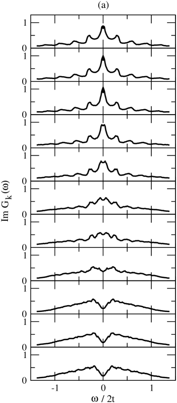
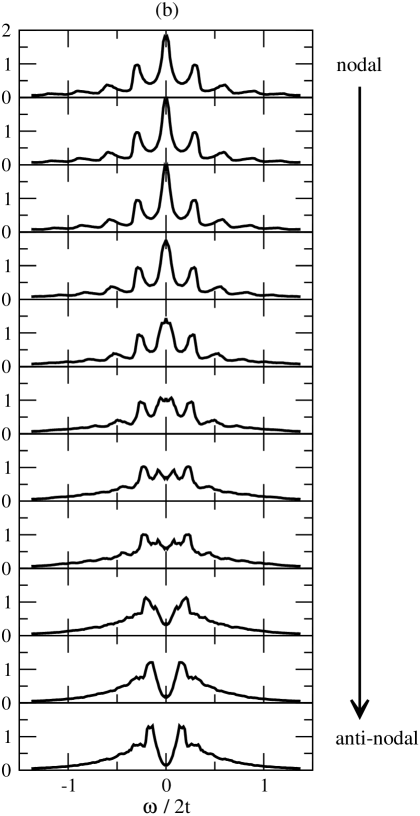
Figure 2: Symmetrized spectral function $\Im G({\bf k},\omega)$ at $T=0$ for two hole fillings (a) $\delta=0.03$ and (b) $\delta=0.075$ along the Fermi surface. The top $\Im G({\bf k},\omega)$ is at the node, whereas the bottom is at the anti-node, as defined in the inset of Fig. 3.

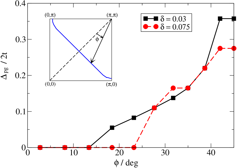
Figure 3: Pseudogap size $\Delta_{pg}$ from Fig. 2 as function of the Fermi surface angle $\phi$ for $\delta=0.03$ (black) and $\delta=0.075$ (red).

Fig. 2 shows the PRM result for $\Im G({\bf k},\omega)$ for two different hole concentrations in the underdoped regime (a) $\delta=0.03$ and (b) $\delta=0.075$, for several $\bf k$-values on the FS between the nodal point near $(\pi/2,\pi/2)$ and the anti-nodal near $(\pi,0)$. As the most important finding, one recognizes the opening of a pseudogap for both hole concentrations, when one proceeds from the nodal towards the anti-nodal direction. On a substantial part of the FS, the spectra show a peak-like behavior around $\omega=0$, indicating a Fermi arc of gapless excitations. Note that our analytical results show a remarkable agreement with findings from ARPES experiments in high-temperature superconductors K06 ; TE07 ; K07 ; K08 . Also additional peaks are found in the nodal direction at lower binding energies which are enhanced for $\delta=0.075$. In Fig. 3, the pseudogap on the FS is shown as a function of the angle $\phi$, where $\phi$ is defined in the inset of Fig. 3. The results are taken from Figs. 2(a) and (b). Note that for the smaller hole filling, the length of the Fermi arc becomes smaller, whereas the pseudogap becomes larger. This behavior agrees with the known experimental feature of a characteristic pseudogap temperature $T^{*}$ which increases with decreasing hole fillingK06 ,TL01 .

The $\omega$- and ${\bf k}$-dependence of $\Im G({\bf k},\omega)$ from Fig. 2 can easily be understood from equation (IV.4),

$$\Im G({\bf k},\omega) = |\tilde{u}_{\bf k}|^{2}D\,\delta(\omega-\varepsilon_{\bf k})$$ (76)

$$+ \frac{3D}{2N^{2}}\sum_{{\bf q}{\bf k}^{\prime}}\left\{\left(\frac{J_{\bf q}}{4\hat{\omega}_{\bf q}^{2}}\right)^{2}|\tilde{v}_{{\bf k},{\bf q}}|^{2}\,\big{(}\varepsilon_{{\bf k}^{\prime}}-\varepsilon_{{\bf k}^{\prime}+{\bf q}}\big{)}^{2}\big{(}\tilde{n}_{{\bf k}^{\prime}+{\bf q}}\tilde{m}_{{\bf k}^{\prime}}+\tilde{n}_{{\bf k}+{\bf q}}(D+\tilde{n}_{{\bf k}^{\prime}}-\tilde{n}_{{\bf k}^{\prime}+{\bf q}})\big{)}\right.$$

$$\qquad+\cdots\Bigg{\}}\,\delta\left(\omega+\varepsilon_{{\bf k}^{\prime}+{\bf q}}-\varepsilon_{{\bf k}^{\prime}}-\varepsilon_{{\bf k}+{\bf q}}\right),$$

where the dots $+\cdots$ indicate additional terms which are less important. First, from the renormalization equation (60) for $u_{{\bf k},\lambda}^{2}$, one finds that its original value $u_{{\bf k}}^{2}=1$ at $\lambda=\Lambda$ is reduced by renormalization contributions of order $\delta^{-2}$ according to $u_{{\bf k},\lambda-\Delta\lambda}^{2}-u_{{\bf k},\lambda}^{2}=-\alpha_{\lambda}/\delta^{2}$. Thus, the weight of the coherent excitation $|\tilde{u}_{{\bf k}}|^{2}$ becomes small for small $\delta$, so that the spectral function $\Im G({\bf k},\omega)$ is dominated by the incoherent excitations in Eq. (76). What remains is to show that the different behavior of $\Im G({\bf k},\omega)$ in the nodal and in the anti-nodal region can be understood solely from the incoherent part of Eq. (76):

First note that the dominant contribution in Eq. (76) at small $\omega$ arises from the small ${\bf q}$-terms in the sum over ${\bf q}$, since in the denominator $\hat{\omega}_{\bf q}^{2}\sim{\bf q}^{2}$. In the numerator, the factor $(\varepsilon_{{\bf k}^{\prime}}-\varepsilon_{{\bf k}^{\prime}+{\bf q}})^{2}$ is also proportional to $q^{2}$, so that the combined prefactor $(J_{\bf q}/4\hat{\omega}_{\bf q}^{2})^{2}(\varepsilon_{{\bf k}^{\prime}}-\varepsilon_{{\bf k}^{\prime}+{\bf q}})^{2}$ behaves as $\sim{\bf q}^{-2}$. However, the small ${\bf q}$ terms do not lead to a divergency in Eq. (76) since the additional renormalization parameter $\tilde{v}_{{\bf k},{\bf q}}^{2}$ also vanishes for ${\bf q}\rightarrow 0$. This behavior can be verified by a close inspection of the renormalization equations (60), (61) for $u_{{\bf k},\lambda}$ and $v_{{\bf k},{\bf q},\lambda}$. Next, let us use the small ${\bf q}$ expansion for the energy difference

$$\varepsilon_{{\bf k}^{\prime}}-\varepsilon_{{\bf k}^{\prime}+{\bf q}}=-2t\big{(}q_{x}\sin{k}_{x}^{\prime}+q_{y}\sin k_{y}^{\prime}\big{)}.$$ (77)

The excitations from the $\delta$-function in Eq. (76) are given by

$$\omega=\varepsilon_{{\bf k}^{\prime}}-\varepsilon_{{\bf k}^{\prime}+{\bf q}}+\varepsilon_{{\bf k}+{\bf q}}\approx\varepsilon_{\bf k}+2t\left\{q_{x}\,(\sin k_{x}-\sin k_{x}^{\prime})+q_{y}\,(\sin k_{y}-\sin k_{y}^{\prime})\right\},$$ (78)

which still depend on ${\bf k}^{\prime}$. There is also a ${\bf k}^{\prime}$-dependent factor in the numerator which contributes to the intensity,

$$(\varepsilon_{{\bf k}^{\prime}}-\varepsilon_{{\bf k}^{\prime}+{\bf q}})^{2}=4t^{2}\big{(}q_{x}\sin{k}_{x}^{\prime}+q_{y}\sin k_{y}^{\prime}\big{)}^{2}+\mathcal{O}(q^{4}).$$ (79)

Now, we are able to discuss the small $\omega$-behavior of the spectral function $\Im G({\bf k},\omega)$, when the wave vector ${\bf k}$ is varied:

(i) First, close to the anti-nodal point ${\bf k}=(0,\pi)$, the excitation energy (78) reduces to

$$\omega=\varepsilon_{{\bf k}^{\prime}}-\varepsilon_{{\bf k}^{\prime}+{\bf q}}+\varepsilon_{{\bf k}+{\bf q}}\approx\varepsilon_{\bf k}-2t\left(q_{x}\,\sin k_{x}^{\prime}+q_{y}\,\sin k_{y}^{\prime}\right).$$ (80)

By comparing Eq. (80) with Eq. (79), one realizes that the square of the frequency shift in Eq. (80) is identical to the intensity factor (79). Thus, excitations with small shifts away from the Fermi surface $\varepsilon_{\bf k}=0$ also have small intensities, whereas those with large shifts have large intensities. This explains naturally the pseudogap behavior at the anti-nodal point, where a lack of intensity is found at $\omega=0$.

(ii) For the nodal point near ${\bf k}=(\pi/2,\pi/2)$, the excitations have energies

$$\omega=\varepsilon_{{\bf k}^{\prime}}-\varepsilon_{{\bf k}^{\prime}+{\bf q}}+\varepsilon_{{\bf k}+{\bf q}}\approx\varepsilon_{\bf k}+2t\left\{q_{x}\,(1-\sin k_{x}^{\prime})+q_{y}\,(1-\sin k_{y}^{\prime})\right\}\,,$$ (81)

whereas the intensity factor is again given by Eq. (79). The largest intensity is caused by terms in the sum over ${\bf k}^{\prime}$ which either belong to the region around ${\bf k}^{\prime}\approx(\pi/2,\pi/2)$ or around ${\bf k}^{\prime}\approx(-\pi/2,-\pi/2)$. In the first case, the excitations (81) reduces to $\omega\approx\varepsilon_{\bf k}$, whereas the intensity factor (79) is given by $4t^{2}(q_{x}+q_{y})^{2}$. Thus, from this ${\bf k}^{\prime}$-region, one obtains excitations directly at the Fermi surface. For the second ${\bf k}^{\prime}$-region, the excitation energies are given by $\omega\approx\varepsilon_{\bf k}+4t(q_{x}+q_{y})$. The intensity factor is the same as before. Thus, similar to the anti-nodal point, the square of the excitation shift away from the Fermi surface $\varepsilon_{\bf k}=0$ is proportional to the corresponding intensity. Therefore, from these ${\bf k}^{\prime}$-terms no intensity is expected at $\omega=0$. To summarize, an excitation peak at $\omega=0$ is expected for wave vectors ${\bf k}$ at the anti-nodal point from the first ${\bf k}^{\prime}$-regime, discussed above. In contrast, for wave vector ${\bf k}$ at the anti-nodal point a pseudogap arises. This explains the pseudogap behavior of the ARPES spectral function and leads to an understanding of the spectra of Fig. 2.

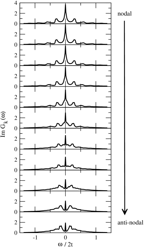
Figure 4: Same quantity as in Figs. 2(a) or (b) for a larger hole doping of $\delta=0.09$.

In Fig. 4, the spectral function is plotted for a larger hole concentration $\delta=0.09$. The remarkable new feature is the occurrence of a narrow coherent excitation at $\omega=0$. Note that for this hole concentration, the weight $D|\tilde{u}_{{\bf k}}|^{2}$ of the coherent excitation is no longer negligible as in the preceding cases since the renormalization contributions $\sim 1/\delta^{2}$ to $u_{{\bf k},\lambda}^{2}$ are less important for larger $\delta$. By increasing $\delta$, the coherent peak gains weight at the expense of the incoherent excitations. We also expect a broadening of the coherent peak due to a coupling to other degrees of freedom such as phonons or impurities.

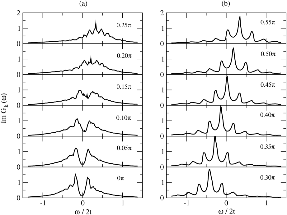
Figure 5: Spectral functions $\Im G({\bf k},\omega)$ for two fixed $k_{x}$ values: (a) $k_{x}=\pi$ and (b) $k_{x}=\pi/2$ and different values of $k_{y}$, thereby crossing the Fermi surface. The hole filling $\delta=0.075$ is the same as in Fig. 2(b).

In Figs. 5(a) and (b), the spectral functions are shown for two different cuts in the Brillouin zone. In both figures, $k_{x}$ is fixed and $k_{y}$ is varied thereby crossing the FS. In panel (a), where $k_{x}=\pi$, the cut runs along the anti-nodal region through the FS at ${\bf k}_{F}\approx(\pi,0.07\pi)$. Note that the pseudogap is restricted to a small $\bf k$-range around the anti-nodal point. It disappears for larger $k_{y}$ values away from the anti-nodal point, in agreement with the earlier discussion on the origin of the pseudogap. The spectra along a cut in the nodal region are shown in panel (b), where $k_{x}=\pi/2$. Apart from the dominant excitation which corresponds to the gapless excitation on the FS in Fig. 2, also weaker excitations are found at lower binding energies. The complete peak structure is shifted almost unchanged through the FS, when $k_{y}$ is varied. The energy distance between the primary and the secondary peak slowly decreases by proceeding along the FS from the nodal point to the anti-nodal point, until finally both peaks disappear when the anti-nodal region is reached. Such a double-peak structure with the same properties along the FS was observed in underdoped cuprate superconductors CSG08 . Finally, one point might still be worth mentioning. For fixed $\omega$, the spectrum in ${\bf k}$-space is much broader than what one would expect for free electrons. Thus, the electron occupation $\langle\hat{c}_{{\bf k}\sigma}^{\dagger}\hat{c}_{{\bf k}\sigma}\rangle=\int d\omega(1+e^{\beta\omega})^{-1}\Im G({\bf k},\omega)$ depends only weakly on ${\bf k}$. This feature is consistent with the former expression (71) for $\tilde{n}_{\bf k}$, where the Gutzwiller approximation was used. Remember that the expectation value $\tilde{n}_{\bf k}$ was defined with the renormalized Hamiltonian $\tilde{\cal H}$ and not with ${\cal H}$.

V.2 Finite temperature results

Next, we discuss the influence of the temperature on the one-particle spectra in the normal state. For the hopping to next nearest neighbors, we use a somewhat larger value $t^{\prime}=0.4t$. This leads to an enhanced curvature of the Fermi surface, as it is observed in most of the copper oxides superconductors. The other parameters remain unchanged.

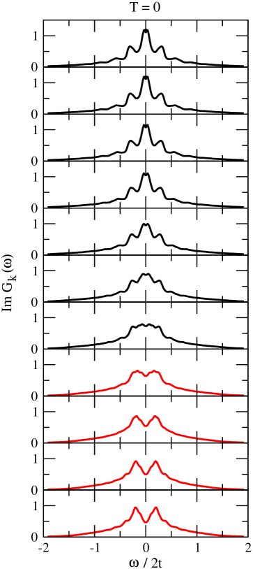
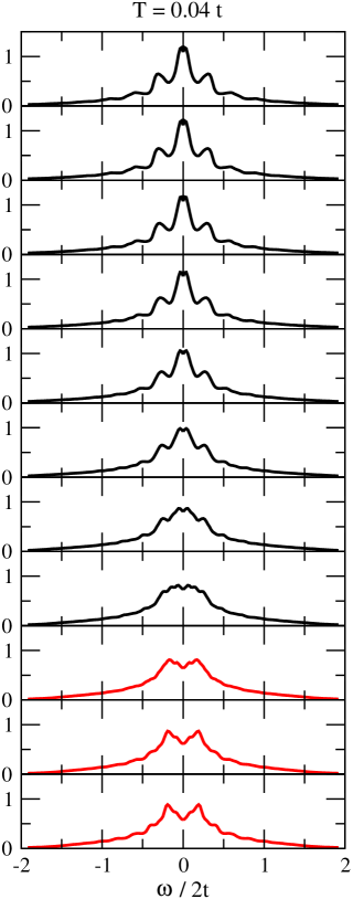
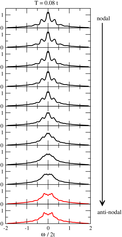
Figure 6: Symmetrized spectral function $\Im G({\bf k},\omega)$ at doping $\delta=0.04$. for three temperatures (a) $T=0$, (b) $T=0.04t$ and (c) $T=0.08t$ for ${\bf k}$-values along the FS. The other parameters are $t^{\prime}=0.4t$ and $J=0.2t$. The top $\Im G({\bf k},\omega)$ is at the node, whereas the bottom is at the anti-node. A possible superconducting solution was suppressed.

Fig. 6 shows the symmetrized spectral function $\Im G({\bf k},\omega)$ for three different temperatures (a) $T=0$, (b) $T=0.04t$, and (c) $T=0.08t$. The hole concentration for all curves is $\delta=0.04$. Possible superconducting solutions are again suppressed. The results are shown for different ${\bf k}$-vectors on the Fermi surface between the nodal (top) and the anti-nodal point (below). For all temperatures, a separation of the Fermi surface into two segments is found, as it was already discussed in the foregoing section: (i) For ${\bf k}$-vectors around the nodal points, $\Im G({\bf k},\omega)$ shows strong excitations at $\omega=0$ (black curves). They form the Fermi arc. (ii) The other segment is given by ${\bf k}$-vectors, for which $\Im G({\bf k},\omega)$ shows a pseudogap around $\omega=0$ (red curves). From Figs. 6(a)-(c), one can see that the length of the Fermi arc increases with increasing temperature. This increase is equivalent to a reduction of the pseudogap region. For instance, for the largest temperature $T=0.08t$, the pseudogap is restriced to a quite small region around the anti-nodal point. Note that this temperature behavior is in good agreement with recent ARPES experimentsK06 . A comparison of the spectral functions at the anti-nodal point for three different temperatures (lowest curves in Figs. 6(a)-(c)) shows the influence of $T$ on the pseudogap: With increasing $T$, the pseudogap is filled up with additional spectral weight, whereas the magnitude of the gap (i.e. the distance between the maxima on the $\omega$-axis) remains almost constant. Also this temperature behavior is verified experimentally K06 . A characteristic temperature $T^{*}$ can be defined at which the pseudogap is completely filled up, and the Fermi arc extends over the whole Fermi surface. This temperature $T^{*}$ was already introduced above and is called pseudogap temperature. For the present case, $T^{*}$ is approximately $T^{*}\approx 0.1t$.

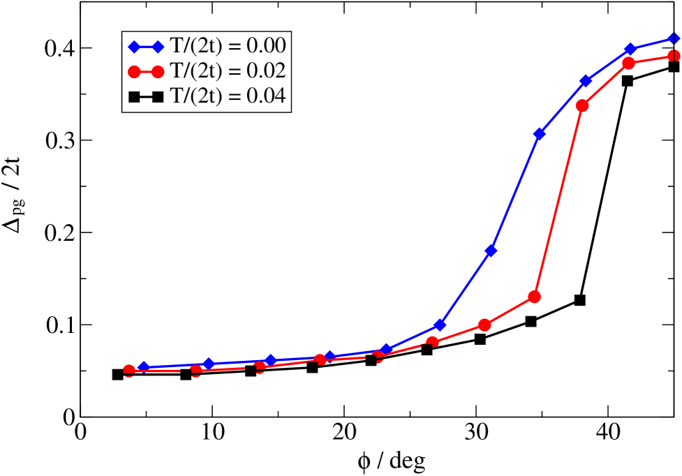
Figure 7: Pseudogap $\Delta_{pg}$ from Fig. 6 as a function of the Fermi surface angle $\phi$ for $T=0$ (blue), $T=0.04t$ (red), and $T=0.08t$ (black).

The pseudogaps, taken over from Figs. 6(a)-(c), are shown in Fig. 7 for three different temperatures as function of the Fermi surface angle $\phi$. Note the strong increase of the pseudogap at a finite Fermi angle which depends on the temperature. This particular angle marks the transition between the Fermi arc and the pseudogap section. At $T=0$, it is about 25 degrees and moves towards the anti-nodal point for higher temperatures. From Fig. 7, one may also deduce that the length of the Fermi arc approximately increases linearly with $T$. Also this feature is consistent with ARPES experimentsK06 .

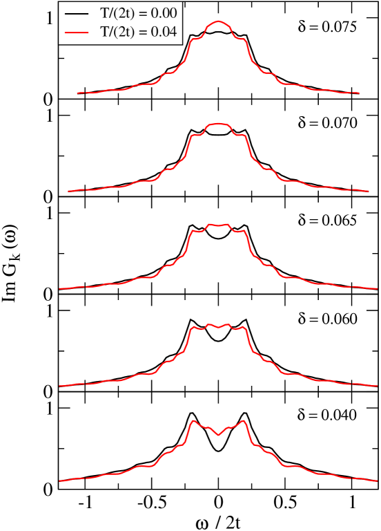
Figure 8: Symmetrized spectral function $\Im G({\bf k},\omega)$ for fixed ${\bf k}$ value on the anti-nodal point for five different hole concentrations from $\delta=0.04$ (bottom curves) to $\delta=0.075$ (top curves). In each case, the results are shown for two different temperatures $T=0$ (black) and $T=0.08t$ (red). For the coherent excitations $\sim|\tilde{u}_{\bf k}|^{2}$, the same broadening has been taken for each $\delta$-value.

To discuss the influence of $\delta$ on the temperature dependence, in Fig. 8 the symmetrized spectral function $\Im G({\bf k},\omega)$ is shown as function of $\omega$ for two different temperatures $T=0$ (black) and $T=0.08t$ (red) and for five different hole concentrations between $\delta=0.04$ (bottom) and $\delta=0.075$ (top). The ${\bf k}$-vector is fixed to the anti-nodal point on the FS. The curves for $T=0$ (black) show a decrease of the pseudogap with increasing hole concentration until it vanishes at $\delta\approx 0.075$. For the higher temperature $T=0.08t$ (red), the pseudogap vanishes already at a lower hole concentration of $\delta\approx 0.06$. This verifies the experimentally known decrease of the pseudogap temperature $T^{*}$ with increasing hole concentration.

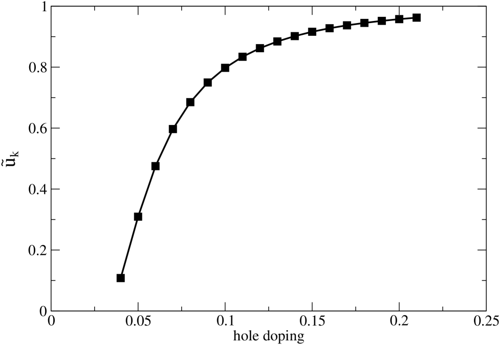
Figure 9: The renormalized amplitude $\tilde{u}_{\bf k}$ of the coherent excitation in Eq. (76) is shown as a function of the hole concentration $\delta$. The ${\bf k}$-vector is fixed to $(0,\pi)$.

The doping and temperature behavior of $\Im G({\bf k},\omega)$ can be understood on the basis of the former result (76) for the spectral function. First, in Fig. 9, the parameter $\tilde{u}_{\bf k}$ is shown as a function of $\delta$ which shows a strong increase with the hole concentration. According to the first line in Eq. (76), $\tilde{u}_{\bf k}$ agrees with the amplitude of the coherent excitation. Therefore, in Fig. 6 for instance, the weight of the coherent excitation $\sim|\tilde{u}_{\bf k}|^{2}$ is negligibly small for the smallest hole concentration $\delta=0.04$, and the spectrum is dominated by the incoherent part of Eq. (76). In contrast, for sufficiently large $\delta$, a coherent excitation at $\omega=0$ is expected, when ${\bf k}$ is fixed to the Fermi surface. This behavior is for instance realized in Fig. 4. Note that an additional broadening of the coherent excitation should be included, which follows from the scattering of the charge carriers at additional phonons or impurities. In Fig. 8, this broadening was assumed to be $T$-independent and was set equal to $0.1t$. Therefore, the following doping behavior can be deduced from Fig. 8: For small hole concentrations $\delta$ ($\delta\ll 0.07$), the spectrum at $T=0$ is dominated by the incoherent excitations with a pronounced pseudogap around the anti-nodal point. For intermediate hole doping ($\delta\approx 0.07$), the spectrum is a superposition of a coherent and of incoherent excitations. Both parts are of the same order of magnitude for an intermediate doping. The incoherent part has still a pseudogap which is partly compensated by the broadening of the coherent excitation. For larger doping $\delta>0.07$, the spectrum mainly consists of a coherent excitation around $\omega=0$. With respect to temperature, the coherent excitation is almost unaffected by $T$, whereas the pseudogap is filled up due to the temperature-dependent shift of the Fermi surface, as will be explained below.

To understand the $T$-behavior of the spectral function, keep in mind that $\tilde{u}_{\bf k}$ and therefore the weight of the coherent excitation in $\Im G({\bf k},\omega)$, is almost independent of $T$. Moreover, the total spectral weight, to which coherent and incoherent excitations contribute, is $T$ independent. This follows from the sum rule (72), since the total electron number is fixed. Thus, except of minor changes, the overall temperature dependence of $\Im G({\bf k},\omega)$ is expected to be weak. Instead, the main reason for the $T$-dependence can be traced back to a change of the Fermi surface with temperature. Consider a ${\bf k}$-vector on the Fermi surface at the anti-nodal point, ${\bf k}_{F}=(\pi,k_{F}^{y})$, where the $x$-component is fixed to $k_{F}^{x}=\pi$. By varying the temperature, one finds that the magnitude of the $y$-component $k_{F}^{y}$ increases almost linearly with $T$. Due to this shift of the Fermi energy with $T$, also the positions of the incoherent excitations at $\omega=0$ are shifted. In this way, one understands that the pseudogap is less pronounced for higher temperatures, when $k_{F}^{x}$ is fixed to $k_{F}^{x}=\pi$. A similar behavior of the pseudogap was found before in Fig. 5. There, the spectral function is shown for fixed $k_{x}=\pi$ and different values of $k_{y}$, when the temperature is fixed. Also in this case, the pseudogap is suppressed for larger values of $k_{y}$. Finally, note that $k_{F}^{y}$ also strongly depends on the nearest-neighbor hopping $t^{\prime}$. For small $t^{\prime}$, the pseudogap is more pronounced than for larger values of $t^{\prime}$. This can be seen by comparing the spectrum in Fig. 2 (with $t^{\prime}=0.1t$) with that of Fig. 6, where $t^{\prime}=0.4t$.

VI Conclusions

In this paper, we have given a microscopic approach to the pseudogap phase in cuprate systems at moderate hole doping. Thereby, a recently developed projector-based renormalization method (PRM) was applied to the $t$-$J$ model. The pseudogap, which is found in ARPES experiments, can be traced back to incoherent excitations in the one-particle Green function. It can neither be explained by a competing order nor as a precursor of superconductivity. Instead, the pseudogap phase is an intrinsic property of the cuprates close to half-filling. In a subsequent paperBS09 , we shall show that a transition to a superconducting phase occurs in the formalism either by lowering the temperature or by approaching an appropriate doping range.

VII Acknowledgements

We would like to acknowledge stimulating and enlightening discussions with J. Fink and A. Hübsch. This work was supported by the DFG through the research program SFB 463.

Appendix A Derivation of the spin susceptibility $\chi({\bf q},\omega)$

The derivation of the spin susceptibility $\chi({\bf q},\omega)$ in Eq. (24) for the system, described by the Hamiltonian ${\cal H}_{0}={\cal H}_{t}+{\cal H}_{J}^{(0)}$, is based on the Mori-Zwanzig projection formalism. This formalism allows to derive exact equations of motion for an appropriately chosen set of relevant operator variables $\{A_{\alpha}\}$,

$$\frac{d}{dt}A_{\alpha}(t) = i\sum_{\beta}A_{\beta}(t)\Omega_{\beta\alpha}-\int_{0}^{t}\sum_{\beta}A_{\beta}(t-t^{\prime})\,\Sigma_{\beta\alpha}(t^{\prime})dt^{\prime}+F_{\alpha}(t)\,,$$ (82)

where the dynamics of the set $A_{\alpha}(t)$ should be governed by ${\cal H}_{0}$, i.e. $A_{\alpha}(t)=e^{\frac{i}{\hbar}{\cal H}_{0}t}A_{\alpha}e^{-\frac{i}{\hbar}{\cal H}_{0}t}$. The quantities $i\omega_{\alpha\beta}$, $\Sigma_{\alpha\beta}(t)$, and $F_{\alpha}(t)$ are called frequency matrix, selfenergy, and random force

$$i\Omega_{\alpha\beta} =\sum_{\gamma}\chi_{\alpha\gamma}^{-1}(A_{\alpha}|\dot{A}_{\beta}), \Sigma_{\alpha\beta}(t) =\sum_{\gamma}\chi_{\alpha\gamma}^{-1}\,(\dot{A}_{\gamma}|{\sf Q}e^{i{\sf QL}_{0}{\sf Q}t}{\sf Q}\dot{A}_{\beta}),$$ (83)

$$F_{\alpha}(t) =i\,e^{i{\sf QL}_{0}{\sf Q}t}{\sf Q}{\sf L}_{0}\,A_{\alpha}.$$

Here, $\dot{A}_{\alpha}$ is the time derivative of $A_{\alpha}$, defined by $\dot{A}_{\alpha}=i\,{\sf L}_{0}A_{\alpha}$, and $\chi_{\alpha\beta}^{-1}$ is the inverse of the susceptibility matrix $\chi_{\alpha\beta}=(A_{\alpha}|A_{\beta})$. In Eqs. (83), we have also introduced a scalar product between operator quantities $A$ and $B$,

$$(A|B) = \int_{0}^{\beta}d\lambda\,\langle A^{\dagger}e^{-\,\lambda{\sf L}_{0}}B\rangle_{0}\,,$$ (84)

where the expectation value $\langle\cdots\rangle_{0}$ is formed with ${\cal H}_{0}$ and ${\sf L}_{0}$ is the Liouville operator, which corresponds to ${\cal H}_{0}$. In $\Sigma_{\alpha\beta}(t)$ the quantity ${\sf Q}$ is a projection operator which projects on the subspace of all operator variables which are ’perpendicular’ to the set $\{A_{\alpha}\}$, i.e.

$${\sf Q} = {\bf 1}-\sum_{\alpha}|A_{\alpha})\chi_{\alpha\beta}^{-1}(A_{\beta}|.$$ (85)

To use the general projection formalism to derive $\chi({\bf q},\omega)$, we have to choose an appropriate set of relevant operator $\{A_{\alpha}\}$. In our case, this set is given by ${\bf S}_{\bf q}$ and its time derivative $\dot{\bf S}_{\bf q}$, i.e.

$$\{A_{\alpha}\} = \{\,{\bf S}_{\bf q},\dot{{\bf S}}_{\bf q}\,\}.$$ (86)

From the equations (82), one easily derives the following two equations:

$$\frac{d}{dt}{\bf S}_{\bf q}(t) = \dot{\bf S}_{\bf q}(t),$$ (87)

$$\frac{d}{dt}\dot{\bf S}_{\bf q}(t) = -\,\omega_{\bf q}^{2}\,{\bf S}_{\bf q}(t)-\int_{0}^{t}dt^{\prime}\,\dot{\bf S}_{\bf q}(t-t^{\prime})\,\Sigma_{\bf q}(t^{\prime})+{\bf F}_{\bf q}(t)\,,$$

where the frequency and the selfenergy in the second equation are given by

$$\omega_{\bf q}^{2} = \frac{(\dot{\bf S}_{\bf q}|\dot{\bf S}_{\bf q})}{({\bf S}_{\bf q}|{\bf S}_{\bf q})},\qquad\qquad\Sigma_{\bf q}(t)=\frac{1}{(\dot{\bf S}_{\bf q}|\dot{\bf S}_{\bf q})}(\ddot{\bf S}_{\bf q}|{\sf Q}\,e^{i{\sf QL}_{0}{\sf Q}t}\,{\sf Q}\ddot{\bf S}_{\bf q})$$ (88)

and the random force is ${\bf F}_{\bf q}(t)=e^{i{\sf QL}_{0}{\sf Q}t}{\sf Q}\ddot{\bf S}_{\bf q}$. The projector ${\sf Q}$ projects perpendicular to ${\bf S}_{\bf q}$ and $\dot{\bf S}_{\bf q}$. In deriving the equations (87), we have also used $(S^{\nu}_{\bf q}|\dot{S}_{\bf q}^{\mu})=i\langle[{S_{\bf q}^{\nu}}^{\dagger},S_{\bf q}^{\mu}]\rangle_{0}=0$ (for all $\nu,\mu=x,y,z$), which follows from the exact relation $(A|{\sf L}_{0}B)=\langle[A^{\dagger},B]\rangle_{0}$. To find the dynamical susceptibility $\chi({\bf q},\omega)$, we multiply both equations (87) with the ’bra’ $({\bf S}_{\bf q}|$ and go over to the Laplace transform. Using $({\bf S}_{\bf q}|{\bf F}_{\bf q})=0$, we obtain

$${\chi}({\bf q},\omega) = \frac{-\omega_{\bf q}^{2}}{\omega^{2}-\omega_{\bf q}^{2}-\,\omega\,\Sigma_{\bf q}(\omega)}\,\chi({\bf q}).$$ (89)

Here, $\chi({\bf q})=(S_{\bf q}|S_{\bf q})$ is the static spin susceptibility and $\Sigma_{\bf q}(\omega)$ is the Laplace transformed selfenergy

$$\Sigma_{\bf q}(\omega) = \frac{1}{(\dot{\bf S}_{\bf q}|\dot{\bf S}_{\bf q})}(\ddot{\bf S}_{\bf q}|{\sf Q}\,\frac{1}{\omega-{\sf QL}_{0}{\sf Q}-i\eta}\,{\sf Q}\ddot{\bf S}_{\bf q}).$$ (90)

To proceed, we have to evaluate the second time derivative $\ddot{\bf S}_{\bf q}$

$$\ddot{\bf S}_{\bf q} = -\frac{1}{\sqrt{N}}\sum_{i\neq l}t^{2}_{il}\,(e^{i{\bf q}{\bf R}_{l}}-e^{i{\bf q}{\bf R}_{i}})\,(\vec{S}_{l}{\cal P}_{0}(i)-\vec{S}_{i}{\cal P}_{0}(l))$$

$$-\frac{1}{2\sqrt{N}}\sum_{\alpha\beta}\sum_{i\neq j}\sum_{j(\neq i\neq l)}\,t_{il}\,t_{lj}\,(e^{i{\bf qR}_{i}}-e^{i{\bf qR}_{l}})$$

$$\times\left\{\vec{\sigma}_{\alpha\beta}\left(\hat{c}_{j\alpha}^{\dagger}\,{\cal D}_{\alpha}(l)\,\hat{c}_{i\beta}+\hat{c}_{j,-\alpha}^{\dagger}S_{l}^{\alpha}\hat{c}_{i\beta}\right)+\vec{\sigma}_{\alpha\beta}^{*}\left(\hat{c}_{i\beta}^{\dagger}\,{\cal D}_{\alpha}(l)\,\hat{c}_{j\alpha}+c_{i\beta}^{\dagger}S_{l}^{-\alpha}\hat{c}_{m,-\alpha}\right)\right\}\,,$$

where only the dominant part of the hopping Hamiltonian ${\cal H}_{t}$ was taken into account. The first term on the right hand side of Eq. (A) enters from a twofold hopping to a neighboring site and back. By replacing the two projectors ${\cal P}_{0}(i)$ and ${\cal P}_{0}(l)$ by their expectation values, we come back to the former equation of motion (22). Therefore, we can conclude that the frequency term $\omega_{\bf q}^{2}$, defined in Eq. (88), agrees with the former frequency term $\hat{\omega}_{\bf q}^{2}$ from Eq. (22),

$$\omega_{\bf q}^{2} = \hat{\omega}_{\bf q}^{2}=2P_{0}(t^{2}_{{\bf q}=0}-t^{2}_{{\bf q}})\geq 0.$$ (92)

The second contribution in Eq. (A) describes a twofold hopping away from the starting site and agrees with the quantity ${\sf Q}\ddot{\bf S}_{\bf q}$ in the selfenergy,

$${\sf Q}\ddot{\bf S}_{\bf q} = -\frac{1}{2\sqrt{N}}\sum_{\alpha\beta}\sum_{i\neq j}\sum_{j(\neq i\neq l)}\,t_{il}\,t_{lj}\,(e^{i{\bf qR}_{i}}-e^{i{\bf qR}_{l}})\times$$

$$\times {\sf Q}\,\left\{\vec{\sigma}_{\alpha\beta}\left(\hat{c}_{j\alpha}^{\dagger}\,{\cal D}_{\alpha}(l)\,\hat{c}_{i\beta}+\hat{c}_{j,-\alpha}^{\dagger}S_{l}^{\alpha}\hat{c}_{i\beta}\right)+\vec{\sigma}_{\alpha\beta}^{*}\left(\hat{c}_{i\beta}^{\dagger}\,{\cal D}_{\alpha}(l)\,\hat{c}_{j\alpha}+c_{i\beta}^{\dagger}S_{l}^{-\alpha}\hat{c}_{m,-\alpha}\right)\right\}.$$

In order to obtain a rough estimate for the selfenergy $\Sigma_{\bf q}(\omega)$, we neglect the spin flip operators in Eq. (A) and replace the local projectors ${\cal D}_{\alpha}(i)$ and ${\cal D}_{\alpha}(l)$ as before by their expectation value $D$. By introducing Fourier transformed quantities, we find

$${\sf Q}\ddot{\bf S}_{\bf q} = \frac{D}{2\sqrt{N}}\sum_{\alpha\beta}\vec{\sigma}_{\alpha\beta}\left((\varepsilon_{{\bf k}+{\bf q}}-\varepsilon_{k})^{2}-2(t^{2}_{{\bf q}=0}-t^{2}_{\bf q})\right)\,{\sf Q}\,\hat{c}_{{\bf k}+{\bf q},\alpha}^{\dagger}\hat{c}_{{\bf k}\beta}.$$ (94)

The selfenergy then reads

$$\Sigma_{\bf q}(\omega) = \frac{D^{2}}{(\dot{\vec{S}}_{\bf q}|\dot{\vec{S}}_{\bf q})}\frac{1}{4N}\sum_{{\bf k}{\bf k}^{\prime}}\sum_{\alpha\beta}\sum_{\alpha^{\prime}\beta^{\prime}}\vec{\sigma}_{\alpha\beta}\cdot\vec{\sigma}_{\alpha^{\prime}\beta^{\prime}}^{*}$$

$$\times [(\varepsilon_{{\bf k}+{\bf q}}-\varepsilon_{\bf k})^{2}-2(t^{2}_{{\bf q}=0}-t^{2}_{\bf q})][(\varepsilon_{{\bf k^{\prime}}+{\bf q}}-\varepsilon_{\bf k^{\prime}})^{2}-2(t^{2}_{{\bf q}=0}-t^{2}_{\bf q})]$$

$$\times (\hat{c}_{{\bf k}+{\bf q},\alpha}^{\dagger}\hat{c}_{{\bf k}\beta}|\,\frac{1}{\omega-{\sf Q}{\sf L}_{0}{\sf Q}-i\eta}\,{\sf Q}\,\hat{c}_{{\bf k^{\prime}}+{\bf q},\alpha^{\prime}}^{\dagger}\hat{c}_{{\bf k^{\prime}}\beta^{\prime}})\,.$$

In the final step, we factorize the two-particle correlation function in Eq. (A) in a product of one-particle Green functions. A straightforward calculation leads for the imaginary part of the selfenergy to

$$\Im\Sigma_{\bf q}(\omega)=\frac{D^{2}}{(\dot{\vec{S}}_{\bf q}|\dot{\vec{S}}_{\bf q})}\frac{3}{2N}\sum_{\bf k}[(\varepsilon_{{\bf k}+{\bf q}}-\varepsilon_{\bf k})^{2}-2(t^{2}_{{\bf q}=0}-t^{2}_{\bf q})]^{2}\,\,\Im M_{\bf k}({\bf q},\omega),$$ (96)

$$\Im M_{\bf k}({\bf q},\omega)=\frac{1-e^{-\beta\omega}}{\beta\omega}\frac{1}{\pi}\int_{-\infty}^{\infty}d\tilde{\omega}\,\frac{\Im G_{{\bf k}}^{(0)}(\omega+\tilde{\omega})}{1+\displaystyle e^{-\beta(\omega+\tilde{\omega})}}\,\frac{\Im G_{{\bf k}+{\bf q}}^{(0)}(\tilde{\omega})}{1+e^{\beta\tilde{\omega}}}\,.$$

Here, $\Im G_{{\bf k}}^{(0)}(\omega)$ is the imaginary part of the one-particle Green function, formed with the Hamiltonian ${\cal H}_{0}$,

$$G_{{\bf k}}^{(0)}(\omega) = i\int_{0}^{\infty}dt\,\langle[\hat{c}_{{\bf k},\alpha}(t),\hat{c}_{{\bf k},\alpha}^{\dagger}]_{+}\rangle_{0}\,\,e^{-i(\omega-i\eta)t}.$$ (97)

Finally, we have to evaluate the denominator $(\dot{\vec{S}}_{\bf q}|\dot{\vec{S}}_{\bf q})$ of $\Sigma_{\bf q}(\omega)$. Proceeding in analogy to the evaluation of $\Sigma_{\bf q}(\omega)$, we find

$$(\dot{\bf S}_{\bf q}|\dot{\bf S}_{\bf q}) = \frac{3}{2N}\sum_{\bf k}(\varepsilon_{{\bf k}+{\bf q}}-\varepsilon_{\bf k})^{2}\,(\hat{c}_{{\bf k}+{\bf q},\alpha}^{\dagger}\hat{c}_{{\bf k}\beta}|\hat{c}_{{\bf k}+{\bf q},\alpha}^{\dagger}\hat{c}_{{\bf k}\beta})$$ (98)

with

$$(\hat{c}_{{\bf k}+{\bf q},\alpha}^{\dagger}\hat{c}_{{\bf k}\beta}|\hat{c}_{{\bf k}+{\bf q},\alpha}^{\dagger}\hat{c}_{{\bf k}\beta})=\int_{-\infty}^{\infty}d\omega\,\frac{1-e^{-\beta\omega}}{\beta\omega}\frac{1}{\pi^{2}}\int_{-\infty}^{\infty}d\tilde{\omega}\,\frac{\Im G_{{\bf k}}^{(0)}(\omega+\tilde{\omega})}{1+\displaystyle e^{-\beta(\omega+\tilde{\omega})}}\,\frac{\Im G_{{\bf k}+{\bf q}}^{(0)}(\tilde{\omega})}{1+e^{\beta\tilde{\omega}}}\,.$$

Appendix B Factorization approximation for $\dot{\bf S}_{{\bf q},\lambda}\dot{\bf S}_{-{\bf q},\lambda}$

The aim of this appendix is to simplify the operator product $\dot{\bf S}_{{\bf q},\lambda}\dot{\bf S}_{-{\bf q},\lambda}$ in the expressions for ${\cal H}_{0,\lambda}$ and ${\cal H}_{1,\lambda}$ from Sec. IV.1,

$${\cal H}_{0,\lambda} = \sum_{\bf q}\frac{J_{\bf q}}{2}\left({\bf S}_{\bf q}\cdot{\bf S}_{-{\bf q}}+\frac{1}{\omega_{{\bf q},\lambda}}\dot{\bf S}_{{\bf q},\lambda}\cdot\dot{\bf S}_{-{\bf q},\lambda}\right),$$

$${\cal H}_{1,\lambda} = \sum_{\bf q}\frac{J_{\bf q}}{2}\left({\bf S}_{\bf q}\cdot{\bf S}_{-{\bf q}}-\frac{1}{\omega_{{\bf q},\lambda}}\dot{\bf S}_{{\bf q},\lambda}\cdot\dot{\bf S}_{-{\bf q},\lambda}\right).$$

This will be done by use of a factorization approximation. Using for the time derivative

$$\dot{\bf S}_{{\bf q},\lambda} = \frac{i}{2\sqrt{N}}\sum_{\alpha\beta}\vec{\sigma}_{\alpha\beta}\sum_{i\neq j}t_{{ij},\lambda}(e^{i{\bf q}{\bf R}_{i}}-e^{i{\bf q}{\bf R}_{j}})\,\hat{c}_{i\alpha}^{\dagger}\hat{c}_{j\beta}$$

we first can rewrite $\dot{\bf S}_{{\bf q},\lambda}\dot{\bf S}_{-{\bf q},\lambda}$ as

$$\dot{\bf S}_{{\bf q},\lambda}\dot{\bf S}_{-{\bf q},\lambda} = \frac{1}{4N}\sum_{\alpha\beta}\sum_{\gamma\delta}(\vec{\sigma}_{\alpha\beta}\cdot\vec{\sigma}_{\delta\gamma})\sum_{i\neq j}t_{{ij},\lambda}(e^{i{\bf q}{\bf R}_{i}}-e^{i{\bf q}{\bf R}_{j}})\times$$ (99)

$$\times\sum_{l\neq m}t_{{lm},\lambda}(e^{-i{\bf q}{\bf R}_{l}}-e^{-i{\bf q}{\bf R}_{m}})\,\hat{c}_{i\alpha}^{\dagger}\hat{c}_{j\beta}\hat{c}_{m\delta}^{\dagger}\hat{c}_{l\gamma}.$$

Using a factorization approximation, the four-fermion operator on the right hand side can be reduced to operators $\hat{c}^{\dagger}_{{\bf k}\sigma}\hat{c}_{{\bf k}\sigma}$ which will lead to a renormalization of $\varepsilon_{\bf k}$. Thereby, we have to pay attention to the fact that the averaged spin operator vanishes ($\langle{\bf S}_{i}\rangle=0$) outside the antiferromagnetic regime. Moreover, all local indices in the four-fermion term of Eq. (99) should be different from each other. This follows from the former decomposition of the exchange interaction into eigenmodes of ${\sf L}_{t}$ in Sec. IV.1, where we have implicitly assumed that the operators $\dot{\bf S}_{{\bf q},\lambda}$ and $\dot{\bf S}_{-{\bf q},\lambda}$ do not overlap in the local space. Otherwise, the decomposition would be much more involved. However, it can be shown that these ’interference’ terms only make a minor impact on the results. For the factorization, we find

$$\dot{\bf S}_{{\bf q},\lambda}\dot{\bf S}_{-{\bf q},\lambda} = \frac{3}{4N}\sum_{i\neq j}t_{{ij},\lambda}(e^{i{\bf q}{\bf R}_{i}}-e^{i{\bf q}{\bf R}_{j}})\sum_{l\neq m}t_{{lm},\lambda}(e^{-i{\bf q}{\bf R}_{l}}-e^{-i{\bf q}{\bf R}_{m}})$$ (100)

$$\times \,\left\{\sum_{\alpha}\langle(\hat{c}_{j\beta}\hat{c}_{m\beta}^{\dagger})_{NL}\rangle\,(\hat{c}_{i\alpha}^{\dagger}\hat{c}_{l\alpha})_{NL}+\sum_{\beta}\langle(\hat{c}_{i\alpha}^{\dagger}\hat{c}_{l\alpha})_{NL}\rangle\,(\hat{c}_{j\beta}\hat{c}_{m\beta})_{NL}\right\},$$

where we have neglected an additional c-number quantity, which enters in the factorization. The attached subscript in $(\cdots)_{NL}$ on the right hand side indicates that the local sites of the operators inside the brackets are different from each other. Note that sums over spin indices in Eq. (99) have already been carried out. Fourier transforming Eq. (100) leads to

$$\dot{\bf S}_{{\bf q},\lambda}\dot{\bf S}_{-{\bf q},\lambda}=-\frac{3}{2N}\sum_{{\bf k}\sigma}(\varepsilon_{{\bf k},\lambda}-\varepsilon_{{\bf k}-{\bf q},\lambda})^{2}\langle(\hat{c}_{{\bf k}-{\bf q}\alpha}^{\dagger}\hat{c}_{{\bf k}-{\bf q}\alpha})_{NL}\rangle\,(\hat{c}_{{\bf k}\sigma}^{\dagger}\hat{c}_{{\bf k}\sigma})_{NL},$$ (101)

where we have defined

$$(\hat{c}_{{\bf k}\sigma}^{\dagger}\hat{c}_{{\bf k}\sigma})_{NL} = \hat{c}_{{\bf k}\sigma}^{\dagger}\hat{c}_{{\bf k}\sigma}-\frac{1}{N}\sum_{{\bf k}^{\prime}}\hat{c}_{{\bf k}^{\prime}\sigma}^{\dagger}\hat{c}_{{\bf k}^{\prime}\sigma}.$$

Using Eq. (101) together with Eq. (51), one is led to the renormalization result (53) of $\tilde{\varepsilon}_{\bf k}^{(0)}$ to first order in $J$.

In the following, let us simplify the notation and suppress the index $\lambda$ in $\dot{\bf S}_{{\bf q},\lambda}$, $\varepsilon_{{\bf k},\lambda}$, and also in $\hat{\omega}_{{\bf q},\lambda}$. With this convention, we shall use the factorization (101) in order to derive the renormalization (IV.3) for ${\varepsilon}_{{\bf k},\lambda}$ in second order in $J$. We start from expression (IV.3) for the renormalized Hamiltonian ${\cal H}_{\lambda-\Delta\lambda}^{(2)}$ in second order

$${\cal H}_{\lambda-\Delta\lambda}^{(2)} = \sum_{\bf q}J_{{\bf q}}\,\left\{\Theta(\lambda-|2\hat{\omega}_{{\bf q},\lambda}|)-\frac{1}{2}\right\}\,[\,X_{\lambda,\Delta\lambda},{\cal A}_{1,\lambda}({\bf q})+{\cal A}_{1,\lambda}^{\dagger}({\bf q})\,]+\sum_{\bf q}J_{{\bf q}}\,[X_{\lambda,\Delta\lambda},{\cal A}_{0,\lambda}]$$ (102)

$$= \sum_{\bf q}J_{\bf q}\Theta_{\bf q}(\lambda,\Delta\lambda)\left(\frac{3}{4}[X_{\lambda,\Delta\lambda}\,,{\bf S}_{\bf q}\cdot{\bf S}_{-{\bf q}}]+\frac{1}{4\hat{\omega}_{\bf q}^{2}}[X_{\lambda,\Delta\lambda}\,,\dot{\bf S}_{\bf q}\cdot\dot{\bf S}_{-{\bf q}}]\right)\,,$$

where in the first line we have already used $[X_{\lambda,\Delta\lambda}\,,{\cal H}_{t,\lambda}]=-\sum_{\bf q}J_{\bf q}\,\Theta_{\bf q}(\lambda,\Delta\lambda)\,({\cal A}_{1,\lambda}({\bf q})+{\cal A}_{1,\lambda}^{\dagger}({\bf q}))$. Next, we have to evaluate the commutators of $X_{\lambda,\Delta\lambda}$ with ${\bf S}_{\bf q}\cdot{\bf S}_{-{\bf q}}$ and $\dot{\bf S}_{\bf q}\cdot\dot{\bf S}_{-{\bf q}}$. Using $[\dot{S}_{-{\bf q}}^{\nu}\,,{S}_{{\bf q}}^{\nu}]=\frac{i}{4N}\sum_{{\bf q}\sigma}(2\varepsilon_{\bf k}-\varepsilon_{{\bf k}+{\bf q}}-\varepsilon_{{\bf k}-{\bf q}})\,\hat{c}_{{\bf k}\sigma}^{\dagger}\hat{c}_{{\bf k}\sigma}$, ($\nu=x,y,z$), and Eq. (39), we find

$$[X_{\lambda,\Delta\lambda}\,,{\bf S}_{\bf q}\cdot{\bf S}_{-{\bf q}}] = \frac{J_{\bf q}}{4\hat{\omega}_{\bf q}^{2}}\,\Theta_{\bf q}(\lambda,\Delta\lambda)\left(\frac{1}{N}\sum_{{\bf k}\sigma}(2\varepsilon_{\bf k}-\varepsilon_{{\bf k}+{\bf q}}-\varepsilon_{{\bf k}-{\bf q}})\langle\hat{c}_{{\bf k}\sigma}^{\dagger}\hat{c}_{{\bf k}\sigma}\rangle\right)\,{\bf S}_{\bf q}\cdot{\bf S}_{-{\bf q}}$$

$$+ \frac{J_{\bf q}}{4\hat{\omega}_{\bf q}^{2}}\,\Theta_{\bf q}(\lambda,\Delta\lambda)\langle{\bf S}_{\bf q}\cdot{\bf S}_{-{\bf q}}\rangle\,\frac{1}{N}\sum_{{\bf k}\sigma}(2\varepsilon_{\bf k}-\varepsilon_{{\bf k}+{\bf q}}-\varepsilon_{{\bf k}-{\bf q}})\;\hat{c}_{{\bf k}\sigma}^{\dagger}\hat{c}_{{\bf k}\sigma},$$

$$[X_{\lambda,\Delta\lambda}\,,\dot{\bf S}_{\bf q}\cdot\dot{\bf S}_{-{\bf q}}] = -\frac{J_{\bf q}}{4\hat{\omega}_{\bf q}^{2}}\,\Theta_{\bf q}(\lambda,\Delta\lambda)\left(\frac{1}{N}\sum_{{\bf k}\sigma}(2\varepsilon_{\bf k}-\varepsilon_{{\bf k}+{\bf q}}-\varepsilon_{{\bf k}-{\bf q}})\langle\hat{c}_{{\bf k}\sigma}^{\dagger}\hat{c}_{{\bf k}\sigma}\rangle\right)\,\dot{\bf S}_{\bf q}\cdot\dot{\bf S}_{-{\bf q}}$$ (103)

$$- \frac{J_{\bf q}}{4\hat{\omega}_{\bf q}^{2}}\,\Theta_{\bf q}(\lambda,\Delta\lambda)\langle\dot{\bf S}_{\bf q}\cdot\dot{\bf S}_{-{\bf q}}\rangle\,\frac{1}{N}\sum_{{\bf k}\sigma}(2\varepsilon_{\bf k}-\varepsilon_{{\bf k}+{\bf q}}-\varepsilon_{{\bf k}-{\bf q}})\;\hat{c}_{{\bf k}\sigma}^{\dagger}\hat{c}_{{\bf k}\sigma}.$$

Note that in (B) already a factorization approximation was used. With the relations (102) and (B), we obtain

$${\cal H}_{\lambda-\Delta\lambda}^{(2)} = 3\sum_{\bf q}(\frac{J_{\bf q}}{4\hat{\omega}_{\bf q}^{2}})^{2}\,\Theta_{\bf q}(\lambda,\Delta\lambda)\left(\left[\frac{1}{N}\sum_{{\bf k}\sigma}(2\varepsilon_{\bf k}-\varepsilon_{{\bf k}+{\bf q}}-\varepsilon_{{\bf k}-{\bf q}})\langle\hat{c}_{{\bf k}\sigma}^{\dagger}\hat{c}_{{\bf k}\sigma}\rangle\right]\,{\bf S}_{\bf q}\cdot{\bf S}_{-{\bf q}}\right.$$

$$\left.+\langle{\bf S}_{\bf q}\cdot{\bf S}_{-{\bf q}}\rangle\,\frac{1}{N}\sum_{{\bf k}\sigma}(2\varepsilon_{\bf k}-\varepsilon_{{\bf k}+{\bf q}}-\varepsilon_{{\bf k}-{\bf q}})\;\hat{c}_{{\bf k}\sigma}^{\dagger}\hat{c}_{{\bf k}\sigma}\right)$$

$$- \sum_{\bf q}(\frac{J_{\bf q}}{4\hat{\omega}_{\bf q}^{2}})^{2}\,\Theta_{\bf q}(\lambda,\Delta\lambda)\left(\left[\frac{1}{N}\sum_{{\bf k}\sigma}(2\varepsilon_{\bf k}-\varepsilon_{{\bf k}+{\bf q}}-\varepsilon_{{\bf k}-{\bf q}})\langle\hat{c}_{{\bf k}\sigma}^{\dagger}\hat{c}_{{\bf k}\sigma}\rangle\right]\,\dot{\bf S}_{\bf q}\cdot\dot{\bf S}_{-{\bf q}}\right.$$

$$\left.+\langle\dot{\bf S}_{\bf q}\cdot\dot{\bf S}_{-{\bf q}}\rangle\,\frac{1}{N}\sum_{{\bf k}\sigma}(2\varepsilon_{\bf k}-\varepsilon_{{\bf k}+{\bf q}}-\varepsilon_{{\bf k}-{\bf q}})\;\hat{c}_{{\bf k}\sigma}^{\dagger}\hat{c}_{{\bf k}\sigma}\right).$$

In a final step, we factorize $\sim\dot{\bf S}_{\bf q}\cdot\dot{\bf S}_{-{\bf q}}$ according to (101),

$${\cal H}_{\lambda-\Delta\lambda}^{(2)} = 3\sum_{\bf q}(\frac{J_{\bf q}}{4\hat{\omega}_{\bf q}^{2}})^{2}\,\Theta_{\bf q}(\lambda,\Delta\lambda)\left(\left[\frac{1}{N}\sum_{{\bf k}\sigma}(2\varepsilon_{\bf k}-\varepsilon_{{\bf k}+{\bf q}}-\varepsilon_{{\bf k}-{\bf q}})\langle\hat{c}_{{\bf k}\sigma}^{\dagger}\hat{c}_{{\bf k}\sigma}\rangle\right]\,{\bf S}_{\bf q}\cdot{\bf S}_{-{\bf q}}\right.$$ (105)

$$\left.\qquad+\langle{\bf S}_{\bf q}\cdot{\bf S}_{-{\bf q}}\rangle\,\frac{1}{N}\sum_{{\bf k}\sigma}(2\varepsilon_{\bf k}-\varepsilon_{{\bf k}+{\bf q}}-\varepsilon_{{\bf k}-{\bf q}})\;\hat{c}_{{\bf k}\sigma}^{\dagger}\hat{c}_{{\bf k}\sigma}\right)$$

$$- \sum_{\bf q}(\frac{J_{\bf q}}{4\hat{\omega}_{\bf q}^{2}})^{2}\,\Theta_{\bf q}(\lambda,\Delta\lambda)\langle\dot{\bf S}_{\bf q}\cdot\dot{\bf S}_{-{\bf q}}\rangle\,\frac{1}{N}\sum_{{\bf k}\sigma}(2\varepsilon_{\bf k}-\varepsilon_{{\bf k}+{\bf q}}-\varepsilon_{{\bf k}-{\bf q}})\;\hat{c}_{{\bf k}\sigma}^{\dagger}\hat{c}_{{\bf k}\sigma}$$

$$+ \frac{3}{2N}\sum_{{\bf q}\sigma}(\frac{J_{\bf q}}{4\hat{\omega}_{\bf q}^{2}})^{2}\,\Theta_{\bf q}(\lambda,\Delta\lambda)\,\left[\frac{1}{N}\sum_{{\bf k}^{\prime}\sigma^{\prime}}(2\varepsilon_{{\bf k}^{\prime}}-\varepsilon_{{\bf k}^{\prime}+{\bf q}}-\varepsilon_{{\bf k}^{\prime}-{\bf q}})\langle\hat{c}_{{\bf k}^{\prime}\sigma^{\prime}}^{\dagger}\hat{c}_{{\bf k}^{\prime}\sigma^{\prime}}\rangle\right]\times$$

$$\qquad\times\sum_{{\bf k}\sigma}(\varepsilon_{\bf k}-\varepsilon_{{\bf k}-{\bf q}})^{2}\langle(\hat{c}_{{\bf k}-{\bf q}\alpha}^{\dagger}\hat{c}_{{\bf k}-{\bf q}\alpha})_{NL}\rangle\,(\hat{c}_{{\bf k}\sigma}^{\dagger}\hat{c}_{{\bf k}\sigma})_{NL}.$$

From (105), the renormalization equatiuon (IV.3) for $\varepsilon_{{\bf k},\lambda-\Delta\lambda}$ can immediately be deduced.

Appendix C Renormalization equations for fermion operators

The aim of this appendix is to derive the renormalization equation for the fermion operator $\hat{c}_{{\bf k}\sigma}(\lambda)=e^{X_{\lambda}}\hat{c}_{{\bf k}\sigma}e^{-X_{\lambda}}$ in second order in $J_{\bf q}$. As before, we shall suppress the index $\lambda$ everywhere in $\dot{\bf S}_{{\bf q},\lambda}$, $\hat{\omega}_{{\bf q},\lambda}$, and $\varepsilon_{{\bf q},\lambda}$ in order to simplify the notation. Let us start from an ansatz for $\hat{c}_{{\bf k}\sigma}(\lambda)$ after all excitations with transition energies larger than $\lambda$ have been integrated out. It reads

$$\hat{c}_{{\bf k}\sigma}(\lambda) = u_{{\bf k},\lambda}\hat{c}_{{\bf k}\sigma}-i\sum_{\bf q}\Theta(|2\hat{\omega}_{\bf q}|-\lambda)\,v_{{\bf k,q},\lambda}\,\frac{J_{\bf q}}{4\hat{\omega}^{2}_{\bf q}}\,[{\bf S_{q}}\cdot\dot{\bf S}_{-{\bf q}}+\dot{\bf S}_{-{\bf q}}\cdot{\bf S}_{{\bf q}},\,c_{{\bf k}\sigma}].$$ (106)

In Eq. (106), the parameters $u_{{\bf k},\lambda}$ and $v_{{\bf k,q},\lambda}$ account for the $\lambda$-dependence. Note that the operator structure in Eq. (106) corresponds to that of the first order expansion for $\hat{c}_{{\bf k}\sigma}(\lambda)\approx\hat{c}_{{\bf k}\sigma}+[X_{\lambda},\hat{c}_{{\bf k}\sigma}]$. Here, $X_{\lambda}$ has the same operator form as the generator $X_{\lambda,\Delta\lambda}$ in Eq. (38). Due to construction, the ${\bf q}$-sum in Eq. (106) only runs over $\bf q$-values with excitation energies $|2\hat{\omega}_{\bf q}|$ larger than $\lambda$. This is assured by the $\Theta$-function in Eq. (106). For simplicity, in the following we agree upon to incorporate the $\Theta$-function in $v_{{\bf k,q},\lambda}$. Thus, we can write

$$\hat{c}_{{\bf k}\sigma}(\lambda) = u_{{\bf k},\lambda}\hat{c}_{{\bf k}\sigma}-i\sum_{\bf q}v_{{\bf k,q},\lambda}\frac{J_{\bf q}}{4\hat{\omega}^{2}_{\bf q}}\,\Big{(}\big{(}[{\bf S_{q}},c_{{\bf k}\sigma}]\cdot\dot{\bf S}_{-{\bf q}}+\dot{\bf S}_{-{\bf q}}\cdot[{\bf S}_{{\bf q}},c_{{\bf k}\sigma}]\big{)}$$ (107)

$$\hskip 142.26378pt+\big{(}{\bf S_{q}}\cdot[\dot{\bf S}_{-{\bf q}},c_{{\bf k}\sigma}]+[\dot{\bf S}_{-{\bf q}},c_{{\bf k}\sigma}]\cdot{\bf S_{q}}\,\big{)}\Big{)}.$$

For the additional renormalization from $\lambda$ to the reduced cutoff $\lambda-\Delta\lambda$, we have

$$\hat{c}_{\bf k\sigma}(\lambda-\Delta\lambda)=e^{X_{\lambda,\Delta\lambda}}\,\hat{c}_{{\bf k}\sigma}(\lambda)\,e^{-X_{\lambda,\Delta\lambda}}=$$ (108)

$$\qquad=u_{{\bf k},\lambda}e^{X_{\lambda,\Delta\lambda}}\hat{c}_{{\bf k}\sigma}e^{-X_{\lambda,\Delta\lambda}}-i\sum_{\bf q}v_{{\bf k,q},\lambda}\frac{J_{\bf q}}{4\hat{\omega}^{2}_{\bf q}}\,e^{X_{\lambda,\Delta\lambda}}[{\bf S_{q}}\cdot\dot{\bf S}_{-{\bf q}}+\dot{\bf S}_{-{\bf q}}\cdot{\bf S}_{{\bf q}},\,c_{{\bf k}\sigma}]e^{-X_{\lambda,\Delta\lambda}},$$

where $X_{\lambda,\Delta\lambda}$ is the generator from Eq. (38),

$$X_{\lambda,\Delta\lambda} = -i\sum_{\bf q}\,\frac{J_{\bf q}}{4\hat{\omega}_{\bf q}}\Theta_{\bf q}(\lambda,\Delta\lambda)\left(\bf S_{\bf q}\,\dot{\bf S}_{-{\bf q}}+\dot{\bf S}_{\bf q}\,{\bf S}_{-{\bf q}}\right).$$

First, let us expand the term $\sim u_{{\bf k},\lambda}$ in Eq. (108),

$$e^{X_{\lambda,\Delta\lambda}}\,\hat{c}_{{\bf k}\sigma}\,e^{-X_{\lambda,\Delta\lambda}} = \hat{c}_{{\bf k}\sigma}+[X_{\lambda,\Delta\lambda}\,,\,\hat{c}_{{\bf k}\sigma}]+\frac{1}{2}[X_{\lambda,\Delta\lambda},[X_{\lambda,\Delta\lambda},\hat{c}_{{\bf k}\sigma}]]+\cdots.$$ (109)

Here, we can combine the second term in Eq. (108) with the second part in Eq. (107),

$$\hat{c}_{\bf k\sigma}(\lambda-\Delta\lambda) = (u_{{\bf k},\lambda}+\cdots)\,\hat{c}_{{\bf k}\sigma}$$

$$- i\sum_{\bf q}(v_{{\bf k,q},\lambda}+u_{{\bf k},\lambda}\,\Theta_{\bf q}(\lambda,\Delta\lambda)+\cdots)\,\frac{J_{\bf q}}{4\hat{\omega}^{2}_{\bf q}}\,[{\bf S_{q}}\cdot\dot{\bf S}_{-{\bf q}}+\dot{\bf S}_{-{\bf q}}\cdot{\bf S}_{{\bf q}},\,c_{{\bf k}\sigma}]+\cdots,$$

where the dots $(+\cdots)$ mean additional contributions from higher order commutators with $X_{\lambda,\Delta\lambda}$. On the other hand, $\hat{c}_{\bf k\sigma}(\lambda-\Delta\lambda)$ should have the same form as the ansatz (106), when $\lambda$ is replaced by $\lambda-\Delta\lambda$,

$$\hat{c}_{\bf k\sigma}(\lambda-\Delta\lambda) = u_{{\bf k},\lambda-\Delta\lambda}\hat{c}_{{\bf k}\sigma}-i\sum_{\bf q}v_{{\bf k,q},\lambda-\Delta\lambda}\frac{J_{\bf q}}{4\hat{\omega}^{2}_{\bf q}}\,[{\bf S_{q}}\cdot\dot{\bf S}_{-{\bf q}}+\dot{\bf S}_{-{\bf q}}\cdot{\bf S}_{{\bf q}},\,c_{{\bf k}\sigma}].$$ (111)

The comparison of Eqs. (111) and (C) immediately leads to the renormalization equation (61) for $v_{{\bf k,q},\lambda}$,

$$v_{{\bf k,q},\lambda-\Delta\lambda} = v_{{\bf k,q},\lambda}+u_{{\bf k},\lambda}\,\Theta_{\bf q}(\lambda,\Delta\lambda),$$ (112)

where we have restricted ourselves to the lowest order contributions in $X_{\lambda,\Delta\lambda}$. Furthermore, we have exploited the very weak $\lambda$-dependency of $\varepsilon_{{\bf k},\lambda}$ and $\hat{\omega}_{{\bf q},\lambda}$.

The renormalization equation for the second parameter $u_{{\bf k},\lambda}$ requires the evaluation of higher order commutators in Eq. (108). Alternatively, we can start from the anti-commutator relation (3)

$$[\hat{c}_{{\bf k}\sigma}^{\dagger}(\lambda),\hat{c}_{{\bf k}\sigma}(\lambda)]_{+}=\frac{1}{N}\sum_{i}e^{X_{\lambda}}{\cal D}_{\sigma}(i)e^{-X_{\lambda}}=\frac{1}{N}\sum_{i}{\cal D}_{\sigma}(i)$$

with ${\cal D}_{\sigma}(i)=1-n_{1,-\sigma}$, where in the last relation $[X_{\lambda},\sum_{i}{\cal D}_{\sigma}(i)]=0$ was used. When we take the average, we obtain

$$\langle[\hat{c}_{{\bf k}\sigma}^{\dagger}(\lambda),\hat{c}_{{\bf k}\sigma}(\lambda)]_{+}\rangle = \langle{\cal D}_{\sigma}(i)\rangle=:D.$$ (113)

In order to evaluate the anti-commutator in Eq. (113), we have to insert the former ansatz (107) for $\hat{c}_{{\bf k}\sigma}(\lambda)$. Here, we make an additional approximation by taking into account only the two first terms in Eq. (107). The remaining terms have explicit spin operators ${\bf S}_{\bf q}$. In the commutator of Eq. (113), they lead to additional contributions with one or two spin operators. Outside the antiferromagnetic phase, no magnetic order is present and also spin correlations are weak. Therefore, it seems reasonable to neglect these terms. Thus, we can approximate $\hat{c}_{{\bf k}\sigma}(\lambda)$ by

$$\hat{c}_{{\bf k}\sigma}(\lambda) = u_{{\bf k},\lambda}\hat{c}_{{\bf k}\sigma}-i\sum_{\bf q}v_{{\bf k,q},\lambda}\frac{J_{\bf q}}{4\hat{\omega}^{2}_{\bf q}}\,\left([{\bf S_{q}},c_{{\bf k}\sigma}]\cdot\dot{\bf S}_{-{\bf q}}+\dot{\bf S}_{-{\bf q}}\cdot[{\bf S_{q}},c_{{\bf k}\sigma}]\right)$$

$$= u_{{\bf k},\lambda}\hat{c}_{{\bf k}\sigma}+\frac{1}{2N}\sum_{\bf q}v_{{\bf k,q},\lambda}\frac{J_{\bf q}}{4\hat{\omega}^{2}_{\bf q}}\,\sum_{\alpha\beta\gamma}(\vec{\sigma}_{\alpha\beta}\cdot\vec{\sigma}_{\sigma\gamma})\sum_{{\bf k}^{\prime}}(\varepsilon_{{\bf k}^{\prime}}-\varepsilon_{{\bf k}^{\prime}+{\bf q}})\,\hat{c}^{\dagger}_{{\bf k}^{\prime}+{\bf q}\alpha}\ \hat{c}_{{\bf k}^{\prime}\beta}\ \hat{c}_{{\bf k}+{\bf q}\gamma}.$$

Inserting Eq. (C) and $\hat{c}_{{\bf k}\sigma}^{\dagger}(\lambda)$ into Eq. (113), we obtain

$$D = |u_{{\bf k},\lambda}|^{2}D+\frac{1}{(2N)^{2}}\sum_{{\bf q}^{\prime}{\bf q}}v_{{\bf k,q}^{\prime},\lambda}^{*}\,v_{{\bf k,q},\lambda}\frac{J_{{\bf q}^{\prime}}}{4\hat{\omega}^{2}_{{\bf q}^{\prime}}}\frac{J_{\bf q}}{4\hat{\omega}^{2}_{\bf q}}\,\sum_{\alpha^{\prime},\beta^{\prime},\gamma^{\prime}}\sum_{\alpha,\beta,\gamma}(\vec{\sigma}_{\beta^{\prime}\alpha^{\prime}}\cdot\vec{\sigma}_{\gamma^{\prime}\sigma})(\vec{\sigma}_{\alpha\beta}\cdot\vec{\sigma}_{\sigma\gamma})\times$$

$$\times\sum_{{\bf k}^{\prime},{\bf k}^{\prime\prime}}(\varepsilon_{{\bf k}^{\prime\prime}}-\varepsilon_{{\bf k}^{\prime\prime}+{\bf q}^{\prime}})\,(\varepsilon_{{\bf k}^{\prime}}-\varepsilon_{{\bf k}^{\prime}+{\bf q}})\,\langle\,[\,\hat{c}_{{\bf k}+{\bf q}^{\prime}\gamma^{\prime}}^{\dagger}\hat{c}_{{\bf k}^{\prime\prime}\beta^{\prime}}^{\dagger}\ \hat{c}_{{\bf k}^{\prime\prime}+{\bf q}^{\prime}\alpha^{\prime}}\,,\,\hat{c}^{\dagger}_{{\bf k}^{\prime}+{\bf q}\alpha}\ \hat{c}_{{\bf k}^{\prime}\beta}\ \hat{c}_{{\bf k}+{\bf q}\gamma}]_{+}\,\rangle.$$

To find the renormalization equation for $u_{{\bf k},\lambda-\Delta\lambda}$, we use the same equation, thereby replacing $\lambda$ by $\lambda-\Delta\lambda$. We then obtain

$$D = |u_{{\bf k},\lambda-\Delta\lambda}|^{2}D+\frac{1}{(2N)^{2}}\sum_{{\bf q}^{\prime}{\bf q}}(v_{{\bf k,q}^{\prime},\lambda}^{*}\,+u_{{\bf k},\lambda}^{*}\Theta_{{\bf q}^{\prime}}(\lambda,\Delta\lambda))\ (v_{{\bf k,q},\lambda}+u_{{\bf k},\lambda}\Theta_{\bf q}(\lambda,\Delta\lambda))\,\frac{J_{{\bf q}^{\prime}}}{4\hat{\omega}^{2}_{{\bf q}^{\prime}}}\frac{J_{\bf q}}{4\hat{\omega}^{2}_{\bf q}}$$

$$\times\sum_{\alpha^{\prime},\beta^{\prime},\gamma^{\prime}}\sum_{\alpha,\beta,\gamma}(\vec{\sigma}_{\beta^{\prime}\alpha^{\prime}}\cdot\vec{\sigma}_{\gamma^{\prime}\sigma})(\vec{\sigma}_{\alpha\beta}\cdot\vec{\sigma}_{\sigma\gamma})$$

$$\times\sum_{{\bf k}^{\prime},{\bf k}^{\prime\prime}}(\varepsilon_{{\bf k}^{\prime\prime}}-\varepsilon_{{\bf k}^{\prime\prime}+{\bf q}^{\prime}})\,(\varepsilon_{{\bf k}^{\prime}}-\varepsilon_{{\bf k}^{\prime}+{\bf q}})\,\langle\,[\,\hat{c}_{{\bf k}+{\bf q}^{\prime}\gamma^{\prime}}^{\dagger}\hat{c}_{{\bf k}^{\prime\prime}\beta^{\prime}}^{\dagger}\ \hat{c}_{{\bf k}^{\prime\prime}+{\bf q}^{\prime}\alpha^{\prime}}\,,\,\hat{c}^{\dagger}_{{\bf k}^{\prime}+{\bf q}\alpha}\ \hat{c}_{{\bf k}^{\prime}\beta}\ \hat{c}_{{\bf k}+{\bf q}\gamma}]_{+}\,\rangle\,,$$

where we have inserted the former renormalization result (112) for $v_{{\bf k,q},\lambda-\Delta\lambda}$. Restricting ourselves to the lowest order contributions in $J_{\bf q}$, we can subtract Eq. (C) from Eq. (C) and obtain the renormalization equation which connects $u_{{\bf k},\lambda-\Delta\lambda}$ with $u_{{\bf k},\lambda}$,

$$|u_{{\bf k},\lambda-\Delta\lambda}|^{2}D = |u_{{\bf k},\lambda}|^{2}D-\frac{1}{(2N)^{2}}\sum_{{\bf q}^{\prime}{\bf q}}\frac{J_{{\bf q}^{\prime}}}{4\hat{\omega}^{2}_{{\bf q}^{\prime}}}\frac{J_{\bf q}}{4\hat{\omega}^{2}_{\bf q}}\sum_{\alpha^{\prime},\beta^{\prime},\gamma^{\prime}}\sum_{\alpha,\beta,\gamma}(\vec{\sigma}_{\beta^{\prime}\alpha^{\prime}}\cdot\vec{\sigma}_{\gamma^{\prime}\sigma})(\vec{\sigma}_{\alpha\beta}\cdot\vec{\sigma}_{\sigma\gamma})$$

$$\times \left\{|u_{{\bf k},\lambda}|^{2}\Theta_{{\bf q}^{\prime}}(\lambda,\Delta\lambda)\Theta_{\bf q}(\lambda,\Delta\lambda)\right.$$

$$+\left.(u_{{\bf k},\lambda}\,v_{{\bf k,q}^{\prime},\lambda}^{*}\,\Theta_{\bf q}(\lambda,\Delta\lambda)+u_{{\bf k},\lambda}^{*}\,v_{{\bf k,q},\lambda}\,\Theta_{{\bf q}^{\prime}}(\lambda,\Delta\lambda))\right\}$$

$$\times \sum_{{\bf k}^{\prime},{\bf k}^{\prime\prime}}(\varepsilon_{{\bf k}^{\prime\prime}}-\varepsilon_{{\bf k}^{\prime\prime}+{\bf q}^{\prime}})\,(\varepsilon_{{\bf k}^{\prime}}-\varepsilon_{{\bf k}^{\prime}+{\bf q}})\,\langle\,[\,\hat{c}_{{\bf k}+{\bf q}^{\prime}\gamma^{\prime}}^{\dagger}\hat{c}_{{\bf k}^{\prime\prime}\beta^{\prime}}^{\dagger}\ \hat{c}_{{\bf k}^{\prime\prime}+{\bf q}^{\prime}\alpha^{\prime}}\,,\,\hat{c}^{\dagger}_{{\bf k}^{\prime}+{\bf q}\alpha}\ \hat{c}_{{\bf k}^{\prime}\beta}\ \hat{c}_{{\bf k}+{\bf q}\gamma}]_{+}\,\rangle.$$

What remains is to evaluate the commutator in Eq. (C). In a final factorization approximation, we find

$$|u_{{\bf k},\lambda-\Delta\lambda}|^{2} = |u_{{\bf k},\lambda}|^{2}-\frac{1}{(2N)^{2}}\sum_{{\bf q}}(\frac{J_{{\bf q}}}{4\hat{\omega}^{2}_{{\bf q}}})^{2}\sum_{\alpha,\beta,\gamma}|\vec{\sigma}_{\alpha\beta}\cdot\vec{\sigma}_{\sigma\gamma}|^{2}$$ (118)

$$\times\Theta_{{\bf q}}(\lambda,\Delta\lambda)\left\{|u_{{\bf k},\lambda}|^{2}+(u_{{\bf k},\lambda}\,v_{{\bf k,q},\lambda}^{*}\,+u_{{\bf k},\lambda}^{*}\,v_{{\bf k,q},\lambda}\,)\right\}$$

$$\times\sum_{{\bf k}^{\prime}}(\varepsilon_{{\bf k}^{\prime}}-\varepsilon_{{\bf k}^{\prime}+{\bf q}})^{2}\,\left\{\,n_{{\bf k}+{\bf q}}(n_{{\bf k}^{\prime}}+D)+n_{{\bf k}^{\prime}+{\bf q}}(m_{{\bf k}^{\prime}}-n_{{\bf k}+{\bf q}})\,\right\}$$

$$+ \frac{1}{(2N)^{2}}\sum_{{\bf q}^{\prime}{\bf q}}\frac{J_{{\bf q}^{\prime}}}{4\hat{\omega}^{2}_{{\bf q}^{\prime}}}\frac{J_{\bf q}}{4\hat{\omega}^{2}_{\bf q}}\sum_{\alpha,\beta,\gamma}(\vec{\sigma}_{\gamma\alpha}\cdot\vec{\sigma}_{\beta\sigma})(\vec{\sigma}_{\alpha\beta}\cdot\vec{\sigma}_{\sigma\gamma})$$

$$\times\big{\{}|u_{{\bf k},\lambda}|^{2}\Theta_{{\bf q}^{\prime}}(\lambda,\Delta\lambda)\Theta_{\bf q}(\lambda,\Delta\lambda)$$

$$+(u_{{\bf k},\lambda}\,v_{{\bf k,q}^{\prime},\lambda}^{*}\,\Theta_{\bf q}(\lambda,\Delta\lambda)+u_{{\bf k},\lambda}^{*}\,v_{{\bf k,q},\lambda}\,\Theta_{{\bf q}^{\prime}}(\lambda,\Delta\lambda))\big{\}}$$

$$\times(\varepsilon_{{\bf k}+{\bf q}}-\varepsilon_{{\bf k}+{\bf q}+{\bf q}^{\prime}})\,(\varepsilon_{{\bf k}+{\bf q}^{\prime}}-\varepsilon_{{\bf k}+{\bf q}^{\prime}+{\bf q}})\,\big{\{}n_{{\bf k}+{\bf q}^{\prime}}\,(n_{{\bf k}+{\bf q}}+D)$$

$$+n_{{\bf k}+{\bf q}+{\bf q}^{\prime}}(m_{{\bf k}+{\bf q}}-n_{{\bf k}+{\bf q}^{\prime}})\big{\}}.$$

Summing over the spin indices and exploiting that $u_{{\bf k},\lambda}$ and $v_{{\bf k},{\bf q},\lambda}$ are real, we arrive at expression (60).

References

- (1) J.G. Bednorz and K.A. Müller, Z. Phys. B 64, 189 (1986).
- (2) J. Corson et al., Nature 398, 221 (1999).
- (3) V.J. Emery and S.A. Kivelson, Nature 374, 434-437 (1995).
- (4) D. Pines, Physica C 282287, 273 (1997).
- (5) M. Randeria, cond-mat 9710223 (1997).
- (6) C.M. Varma, Phys. Rev. B 55, 14554 (1997).
- (7) M.R. Norman et.al., Nature (London) 392, 157 (1998).
- (8) K.M. Shen, F. Ronning, D.H. Lu, F. Baumberger, N.J.C. Ingle, W.S. Lee, W. Meevasana, Y. Kohsaka, M. Azuma, M. Takano, H. Takagi, Z.-X. Shen, Science 307, 901 (2005).
- (9) A. Kanigel et al., Nature Phys. 2, 447 (2006).
- (10) K. Terashima et al., Phys. Rev. Lett. 99, 017003 (2007).
- (11) A. Kanigel et al., Phys. Rev. Lett. 99, 157001 (2007).
- (12) A. Kanigel et al., Phys. Rev. Lett. 101, 137002 (2008).
- (13) J. Chang et al., New Journal of Physics 10, 103016 (2008).
- (14) H. Ding, T. Yokoya, J.C. Campuzano, T. Takahashi, M. Randeria, M.R. Norman, T. Mochikuparallel, K. Kadowakiparallel, and J. Giapintzakis, Nature (London) 382, 51 (1996).
- (15) A.G. Loeser, Z.-X. Shen, D.S. Dessau, D.S. Marshall, C.H. Park, P. Fournier, A. Kapitulnik, Science 273, 325 (1996).
- (16) K.W. Becker, A. Hübsch, and T. Sommer, Phys. Rev. B 66, 235115 (2002); for a review see A. Hübsch, S. Sykora, and K.W. Becker, cond-mat 0809.3360 (2008).
- (17) A. Hübsch and K.W. Becker, Eur. Phys. J. B 33, 391 (2003)
- (18) S. Sykora and K.W. Becker, Microscopic approach to high-temperature superconductors: Superconducting phase, to be published.
- (19) P. Fazekas in Lecture Notes on Electron Correlations and Magnetism, World Scientific, Singapore, New Jersey, London, Hongkong, 1999.
- (20) K. Seiler, C. Gros, T.M. Rice, K. Ueda, and D. Vollhardt, J. Low Temp. Phys. 64, 195 (1986).
- (21) J.L: Tallon and J.W. Loram, Physica 249C, 53 (2001).