Indirect Hamiltonian Identification through a small gateway

Abstract

Identifying the nature of interactions in a quantum system is essential in understanding any physical phenomena. Acquiring information on the Hamiltonian can be a tough challenge in many-body systems because it generally requires access to all parts of the system. We show that if the coupling topology is known, the Hamiltonian identification is indeed possible indirectly even though only a small gateway to the system is used. Surprisingly, even a degenerate Hamiltonian can be estimated by applying an extra field to the gateway.

I Introduction

When studying any quantum mechanical system, precise knowledge of its nature is crucially important. In quantum mechanics, any observable phenomena can be explained rigorously, in principle, if we have complete knowledge of the system. More specifically, we need to identify the states of the system, and the Hamiltonian that governs their dynamics. Thus, the acquisition of all the relevant information on the states and Hamiltonian is essential in understanding how nature behaves. The system of interest may include literally everything quantum mechanical, from high Tc superconductors to microscopic structures in nanotechnology or even some highly complex processes in microbiology.

The full information acquisition is, however, in general very hard from an operational as well as from a computational and mathematical point of view, even for small systems Schirmer2009 ; Schirmer2008 ; Young2008 . For large many-body systems spectroscopy reveals only little information about the Hamiltonian, and generally local addressing of its components is required in order to obtain details about the system. Spins which can be controlled individually operate as a gateway, through which we can access and manipulate the system. A common dilemma is that such a gateway not only allows us to interact with the system, but also introduces noise to it. From a Hamiltonian identification perspective, it is therefore crucial to find minimal gateways that suffice to obtain full knowledge on the system. While this is impossible to answer for generic systems, bounds can be derived if the topology of the system is known. In this context, some positive results have been presented for the case of 1-dimensional (1D) chains of spin-1/2 particles Burgarth2009 ; Franco2009 . That is, the coupling strengths between neighboring spins can be estimated by accessing only the spin at the end of the chain. Since schemes to initialize the state of spins as $|\downarrow\downarrow...\downarrow\rangle$ by operating on the chain end are known Burgarth2007c , such identification of the Hamiltonian is sufficient to determine the dynamics of the system completely. These results are of interest in their own right, yet they were limited to the simplest of networks, i.e., 1D chains.

In this paper, we suggest an estimation scheme for general graphs of spins. As well as the details of the Hamiltonian identification procedure, we give a precise condition for the “gateway” (accessible region) that suffices to make the identification possible. For the important cases of finite 2D/3D lattices such a gateway is given by one edge or one face of the lattice, respectively. This is remarkable because the ratio between the gateway size and the unknown parameters is much higher than in the 1D case. We will also show that while in the 1D case the decay properties of the state in the gateway can identify the Hamiltonian, in the 2D case we need its decay properties as well as the transport properties within the gateway. Interestingly, our general condition turns out to coincide with the criterion for the controllability of spin networks Burgarth2008 . Our results here thus indicate that Hamiltonian-identifiable systems are quantum-controllable and vice versa. Furthermore, they support the physical relevance of the topological properties discussed later.

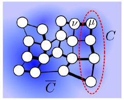
Figure 1: All coupling strengths (black lines) and local magnetic fields (blue background) of a 2-dimensional network $G=(V,E)$ of spins (white circles) can be estimated indirectly by quantum state tomography on a gateway $C$ (enclosed by the dashed red line). The coupling strengths and field intensities are represented by the width of lines and the depth of the background color, respectively. The labeled spins $\mu$ and $\nu$ are used as examples in the proof of the main theorem.

We will study a network with Heisenberg-type interaction. This allows us to describe an estimation procedure that is numerically stable, mathematically simple, and efficient (given that we consider arbitrary and large systems). What we attempt to estimate are the coupling strengths between interacting spins and the strengths of local magnetic fields. Such inhomogeneous fields are very common in experiments, and can cause much trouble through dephasing. Hence it is worthwhile estimating them (such analysis was lacking in Burgarth2009 ; Franco2009 ). Another interesting new aspect we introduce in this paper is how to lift degeneracies on the system by applying extra fields on the gateway. We show that this is always possible, a result which might be relevant beyond the scope of estimation.

Our setup is an example of inverse problems that have been actively studied in plenty of fields in science and engineering. A classical counterpart among those problems that is closest to our quantum setting may be the estimation of spring constants in 1D harmonic oscillator chains Gladwell2004 . However, the resolution to this (classical) problem for generic graphs, even the 2D case, is still open. It would be intriguing if our results in a purely quantum setting could provide some clues to the analogous problem in classical settings.

II Setup and Main Result

Suppose that we have a network of spin-1/2 particles, such as the one in Fig 1. We assume that we have knowledge of the graph $G=(V,E)$, which describes the network: nodes $V$ of the graph correspond to spins and edges $E$ connect spins that are interacting with each other. The pairwise interaction between spins is Heisenberg type with a known anisotropy $\Delta,$ and there is an inhomogeneous magnetic field applied on the spins. Then, the Hamiltonian we consider has the form

$$H = \sum_{(m,n)\in E}c_{mn}\left(\sigma_{m}^{x}\sigma_{n}^{x}+\sigma_{m}^{y}\sigma_{n}^{y}+\Delta\sigma_{m}^{z}\sigma_{n}^{z}\right)+\sum_{n\in V}b_{n}\sigma_{n}^{z},$$

where $c_{mn}$ represent the unknown coupling strengths between spins $m$ and $n$, and $b_{n}$ the unknown intensity of the magnetic field at $n$, respectively. Here, we also assume $c_{mn}<0$ for all $m$ and $n$, i.e., ferromagnetic interactions, though the setup is readily generalized to other cases. In the above, $\sigma_{n}^{i}\>(i={x,y,z})$ are the standard Pauli matrices. The purpose of the following will be to estimate $c_{mn}$ and $b_{n}$ over the entire set $V$ of spins by only accessing a small gateway, described by a subset $C\subset V$ (See Fig. 1). For almost all practical cases of the Hamiltonian identification problem, analyzing the dynamics in the single excitation sector $\mathcal{H}_{1}$ turns out to be sufficient. We will thus denote a single excitation state as $|\mathbf{n}\rangle\in\mathcal{H}_{1}$ when the spin $n\in V$ is in the state $|\uparrow\rangle$ and all others are in $|\downarrow\rangle$ for clarity. The state with all spins in $|\downarrow\rangle$ will be written as $|\mathbf{0}\rangle.$

Naturally, the nice challenge here is to obtain information about the inaccessible spins $\overline{C}\equiv V\backslash C$, which could be the large majority of the set. The question is however how small can the controlled $C$ be such that we can (in principle) still learn all the couplings and fields in $V?$ Intuitively the knowledge of the graph structure can be useful for making the estimation efficient. For instance, the smaller the number of non-vanishing couplings $|E|,$ the more efficiently we can estimate them. However the efficiency should also depend on the structural property of the graph.

To answer this question, we need to introduce a property, known as infecting, of a subset $C\subset V$ of the nodes Burgarth2007 ; Burgarth2008 ; Severini2008 ; Alon . In many-body quantum mechanics this property has many interesting consequences on the controllability and on relaxation properties of the system Burgarth2007 ; Burgarth2008 . The infection process can be described as follows. Suppose that a subset $C$ of nodes of the graph is “infected” with some property. This property then spreads, infecting other nodes, by the following rule: an infected node infects a “healthy” (non-infected) neighbor if and only if it is its unique healthy neighbor. If eventually all nodes are infected, the initial set $C$ is called infecting. The graph in Fig. 1 is an example in which $C$ infects $V$ (we encourage the reader to confirm this by coloring the nodes in region $C$ and applying the above propagation rule — this will make the following proof much more intuitive). With this definition, we can summarize the main result of the paper as the following

Theorem:

Assume that that $C$ infects $V.$ Then all $c_{nm}$ and $b_{n}$ can be obtained by acting on $C$ only.

This theorem provides an upper bound on the smallest number of spins we need to access in order to perform Hamiltonian tomography, i.e. given by the cardinality $|C|$ of the smallest set $C$ that infects $V.$ To prove the above statement, we first present a lemma and its proof.

Lemma:

Assume that $C$ infects $V$ and that all eigenvalues $E_{j}$ $(j=1,\ldots,|V|$) in $\mathcal{H}_{1}$ are known. Assume that for all orthonormal eigenstates $|E_{j}\rangle$ in $\mathcal{H}_{1}$ the coefficients $\langle\mathbf{n}|E_{j}\rangle$ are known for all $n\in C.$ Then the $c_{nm}$ and $b_{n}$ are known.

While the assumptions of the lemma may sound unrealistic, we will show later how they can be obtained by simple tomography experiments on $C.$

Proof of the Lemma:

We observe that the coupling strengths between spins within $C$ are easily obtained because of the relation

$$c_{mn}=\langle\mathbf{m}|H|\mathbf{n}\rangle=\sum E_{k}\langle\mathbf{m}|E_{k}\rangle\langle E_{k}|\mathbf{n}\rangle,$$ (1)

where we defined $c_{mm}\equiv\langle\mathbf{m}|H|\mathbf{m}\rangle$ for the diagonal terms. Since $C$ infects $V$ there is a $\mu\in C$ and a $\nu\in\overline{C}\equiv V\backslash C$ such that $\nu$ is the only neighbor of $\mu$ outside of $C,$ i.e.

$$\langle\mathbf{n}|H|\bm{\mu}\rangle=0\;\;\forall n\in\overline{C}\backslash\{\nu\}.$$ (2)

For an example see Fig. 1. Using the eigenequation, we obtain for all $j$

$$E_{j}|E_{j}\rangle=H|E_{j}\rangle=\sum_{m\in C}\langle\mathbf{m}|E_{j}\rangle H|\mathbf{m}\rangle+\sum_{n\in V\backslash C}\langle\mathbf{n}|E_{j}\rangle H|\mathbf{n}\rangle.$$

Multiplying with $\langle\bm{\mu}|$ and using Eq. (2) we obtain

$$E_{j}\langle\bm{\mu}|E_{j}\rangle-\sum_{m\in C}c_{\mu m}\langle\mathbf{m}|E_{j}\rangle=c_{\mu\nu}\langle\bm{\nu}|E_{j}\rangle.$$ (3)

By assumption and by Eq. (1), the left-hand side (LHS) is known for all $j.$ This means that up to an unknown constant $c_{\mu\nu}<0$ the expansion of $|\bm{\nu}\rangle$ in the basis $|E_{j}\rangle$ is known. Through normalization of $|\mathbf{\bm{\nu}}\rangle$ we then obtain $c_{\mu\nu}$ and hence $\langle\bm{\nu}|E_{j}\rangle$. Redefining $C\Rightarrow C\cup\{\mu\}$, it follows by induction that all $c_{mn}$ are known. Finally, we have

$$c_{mm}=\langle\mathbf{m}|H|\mathbf{m}\rangle=E_{0}-\Delta\sum_{n\in N(m)}c_{mn}+2b_{m},$$ (4)

where $N(m)$ stands for the (directly connected) neighborhood of $m,$ and

$$E_{0}=\frac{1}{2}\Delta\sum_{(m,n)\in V}c_{mn}-\sum_{n\in V}b_{n}$$ (5)

is the energy of the ground state $|\mathbf{0}\rangle$. Summing Eq. (4) over all $m\in V$ and using Eq. (5), we can have the value of $\sum_{n\in V}b_{n}$, thus that of $E_{0}$ as well, since all other parameters are already known. Then we obtain the strength of each local magnetic field, $b_{m}$, from Eq. (4). $\blacksquare$

III Tomography

Let us now describe how to obtain the information that is assumed to be known in the lemma. That is, we need to know the energy eigenvalues $E_{j}$ in $\mathcal{H}_{1}$ and the coefficients $\langle\mathbf{n}|E_{j}\rangle$ for all $n\in C$ by controlling/measuring the spins in $C$. Let us first consider the case where the eigenvalues in $\mathcal{H}_{1}$ are non-degenerate. The general case will be described in Section IV. To start the estimation, we initialize the system as $\frac{1}{\sqrt{2}}(|\mathbf{0}\rangle+|\mathbf{1}\rangle).$ As discussed in Burgarth2007c this can be done efficiently by acting on region $C$ only. Then, we perform quantum state tomography on the spin $n\in C$ after a time lapse $t$. The entire state at $t$ is now

$$\frac{1}{\sqrt{2}}U(t)(|\mathbf{0}\rangle+|\mathbf{1}\rangle)=\frac{1}{\sqrt{2}}\left(e^{-iE_{0}t}|\mathbf{0}\rangle+\sum_{n=1}^{|V|}f_{n1}(t)|\mathbf{n}\rangle\right),$$

where $f_{n1}=\langle\mathbf{n}|U(t)|\mathbf{1}\rangle$ are the elements of the time evolution operator in the single excitation subspace. By repeating the preparation and tomographic measurements on spin $n$ for various times $t$, we obtain the following matrix elements of the time evolution operator as a function of $t:$

$$e^{iE_{0}t}\langle\mathbf{n}|U(t)|\mathbf{1}\rangle=\sum_{j}\langle\mathbf{n}|E_{j}\rangle\langle E_{j}|\mathbf{1}\rangle e^{-i(E_{j}-E_{0})t}.$$ (6)

If we take $n=1$ and Fourier transform Eq. (6) we can get information on the energy spectrum of the Hamiltonian in $\mathcal{H}_{1}$. Up to an unknown constant $E_{0}$, which will turn out to be irrelevant later, we learn the values of those $E_{j}$ corresponding to eigenstates that have non-zero overlap with $|\mathbf{1}\rangle.$ We also obtain the values of $|\langle\mathbf{1}|E_{j}\rangle|^{2}$ for all eigenstates. Due to the freedom in determining the overall phase of a state, we can assume that the coefficients for $|\mathbf{1}\rangle$ of all $|E_{j}\rangle$ are real and positive, $\langle\mathbf{1}|E_{j}\rangle>0.$ Hence observing the decay/revival of an excitation at $n=1$ we can already learn some $E_{j}$ and all the $\langle\mathbf{1}|E_{j}\rangle$. This is analogous to the $1D$ case, where this knowledge would suffice to obtain the full Hamiltonian Burgarth2009 .

In arbitrary graphs however this is no longer the case. In fact even if we observed the decay/revival at each $n\in C$ we would only obtain the $\left|\langle\mathbf{n}|E_{j}\rangle\right|^{2},$ but could not determine their phase freely anymore. To obtain the required knowledge for the Lemma, we need to observe the transport within $C.$ This is represented by Fourier transforming Eq. (6) for $n\neq 1,$ allowing us to extract the coefficient $\langle\mathbf{n}|E_{j}\rangle$ correctly, including their relative phase with respect to $\langle\mathbf{1}|E_{j}\rangle$. We also obtain those eigenvalues $E_{j}$ which have non-zero overlap with $|\mathbf{n}\rangle.$ Continuing this analysis over all elements of $C,$ we learn all eigenvalues which have overlap with some $n\in C.$ Could there be eigenstates in $\mathcal{H}_{1}$ which have no overlap with any $n\in C$? The answer is no, as it is shown in Burgarth2007 . Therefore we can conclude that all eigenvalues in the $\mathcal{H}_{1}$ can be obtained.

Although tomography cannot determine the extra phase shift $E_{0},$ it does not affect the estimation procedure. There are three equations that seem to require the explicit values of $E_{j}$, namely Eq. (1) for $c_{mn}$ inside $C,$ Eq. (3) for $c_{\tilde{m}\tilde{n}}$ and coefficients $\langle\tilde{\mathbf{n}}|E_{j}\rangle$ for a spin outside $C,$ and Eq. (4) for the magnetic fields. It is straightforward to see that for $m\neq n$ substituting $E_{j}-E_{0}$ into $E_{j}$ in Eq. (1) gives the correct $c_{mn}.$ Similarly, the invariance of Eq. (4) is clear as it only depends on $E_{j}-E_{0}$. Less obvious is Eq. (3), however, the key is that the summation over $m\in C$ contains the diagonal term $c_{\mu\mu}=\langle\boldsymbol{\mu}|H|\mathbf{\boldsymbol{\mu}}\rangle=\sum_{j}E_{j}|\langle\boldsymbol{\mu}|E_{j}\rangle|^{2}.$ Then, by substituting $E_{j}-E_{0}$ into $E_{j}$ in the LHS of Eq. (3), it is straightforward to confirm that $E_{0}$ cancels out. Therefore, the precise value of $E_{0}$ is not necessary for the Hamiltonian identification. Eventually, $E_{0}$ can be calculated by Eq. (5) after having all $c_{mn}$ and $b_{n}$.

IV Efficiency and Degeneracy

The efficiency analysis of the Hamiltonian tomography is roughly the same as in Burgarth2009 . Due to the conservation of excitations, the sampling can be restricted to an effective $|V|$- dimensional Hilbert space, and the speed is some polynomial in $|V|,$ provided localization is negligible. One difference however is that in arbitrary graphs it might be less likely that the spectrum is non-degenerate. An explicit example can be given for a square lattice with equal coupling strengths, with the spectrum $E_{kj}=E_{k}+E_{j},$ $k,j=1,...,N,$ where the $E_{k}$ the $1D$ energies of the corresponding chain. A uniform $1D$ system on the other hand would typically be non-degenerate. Of course "exact degeneracy" is highly unlikely; however approximate degeneracy could make the scheme less efficient. Here, we suggest to lift degeneracies by applying extra fields on the gateway $C.$ Since $C$ is only a small subset of the spin, it is not obvious at all that this is possible. We prove the following perhaps startling property of the infection property:

Theorem:

Assume that $C$ infects $V.$ Then there exists an operator $B_{C}$ on $C$ that lifts all degeneracies of $H$ in the single excitation subspace.

Proof:

We will prove the above by explicitly constructing a $B_{C}$ that does the job. This $B_{C}$ will be very inefficient and even requires full knowledge of the Hamiltonian, but is only introduced here for the sake of this proof. Let us denote the eigenvalues of $H$ as $E_{k}$ and the eigenstates as $|E_{k}^{d}\rangle,$ where $d=1,\ldots,D(k)$ is a label for the $D(k)$-fold degenerate states. Let us first concentrate on one specific eigenspace $\left\{|E_{k}^{d}\rangle,d=1,\ldots,D(k)\right\}$ corresponding to an eigenvalue $E_{k}.$ Since the eigenstates considered here are in the single excitation subspace, we can always decompose them as

$$|E_{k}^{d}\rangle_{C\bar{C}}=|\bm{\phi}_{k}^{d}\rangle_{C}\otimes|\bm{0}\rangle_{\bar{C}}+|\bm{0}\rangle_{C}\otimes|\bm{\psi}_{k}^{d}\rangle_{\bar{C}},$$ (7)

where we introduced the unnormalized states $|\bm{\phi}_{k}^{d}\rangle_{C}$ and $|\bm{\psi}_{k}^{d}\rangle_{\bar{C}}$ in the single excitation subspace of $C$ and $\overline{C},$ respectively. As shown in Burgarth2007 we know that $|\bm{\phi}_{k}^{d}\rangle_{\bar{C}}\neq 0\>\forall d$. This is because if there was an eigenstate in the form of $|\bm{0}\rangle_{C}\otimes|\bm{\psi}_{k}^{d}\rangle_{\bar{C}}$ then applying $H$ repeatedly on it will necessarily introduce an excitation to the region $C,$ in contradiction to being an eigenstate. In fact the set $\left\{|\bm{\phi}_{k}^{d}\rangle_{C},\,d=1,\ldots,D(k)\right\}$ must be linearly independent: for, if it was linearly dependent, there would be complex numbers $\alpha_{kd}$ such that $\sum_{d}\alpha_{kd}|\bm{\phi}_{k}^{d}\rangle_{C}=0,$ and because the eigenstates are degenerate, $\sum_{d}\alpha_{kd}|E_{k}^{d}\rangle_{C\bar{C}}=\sum_{d}\alpha_{kd}|\bm{0}\rangle_{C}\otimes|\bm{\psi}_{k}^{d}\rangle_{\bar{C}}$ would be an eigenstate with no excitation in $C,$ again contradicting Ref. Burgarth2007 . This leads to an interesting observation that the degeneracy of each eigenspace can be maximally $|C|-$fold, because there can be only $|C|$ linearly independent vectors at most in the single excitation sector on $C.$ Thus minimal infecting set of a graph gives us some bounds on possible degeneracies.

Now we consider a Hermitian perturbation $B_{kC}\otimes\openone_{\bar{C}}$ (to be specified later) on the system and compute the shift in energies. We shall see that it suffices to assume that $B_{kC}|\mathbf{0}\rangle_{C}=0.$ In first order, we need to compute the eigenvalues of the perturbation matrix

$${}_{C\bar{C}}\langle E_{k}^{d}|B_{kC}|E_{k}^{d^{\prime}}\rangle_{C\bar{C}}=_{C}\langle\bm{\phi}_{k}^{d}|B_{kC}|\bm{\phi}_{k}^{d^{\prime}}\rangle_{C}.$$ (8)

Can we find a $B_{kC}$ such that all eigenvalues differ? For that, note that $\left\{|\bm{\phi}_{k}^{d}\rangle_{\bar{C}},\,d=1,\ldots,D(k)\right\}$ are linearly independent, which means that there is a similarity transform $S_{k}$ (not necessarily unitary, but invertible) such that the vectors $|\bm{\xi}_{k}^{d}\rangle_{C}\equiv S_{k}^{-1}|\bm{\phi}_{k}^{d}\rangle_{C}$ are orthonormal. The perturbation matrix can then be written as ${}_{C}\langle\bm{\xi}_{k}^{d}|S_{k}^{\dagger}B_{kC}S_{k}|\bm{\xi}_{k}^{d^{\prime}}\rangle_{C}.$ If we set

$$S_{k}^{\dagger}B_{kC}S_{k}=\sum_{d}\epsilon_{kd}|\bm{\xi}_{k}^{d}\rangle_{C}\langle\bm{\xi}_{k}^{d}|$$

we can see that the Hermitian operator $B_{kC}\equiv\sum_{d}\epsilon_{kd}\left(S_{k}^{\dagger}\right)^{-1}|\bm{\xi}_{k}^{d}\rangle_{C}\langle\bm{\xi}_{k}^{d}|S_{k}^{-1}$ gives us energy shifts $\epsilon_{kd}.$ Therefore, as long as we choose the $\epsilon_{kd}$ mutually different from each other, the degeneracy in this eigenspace is lifted by $B_{kC}.$ This happens for an arbitrarily small perturbation $\lambda_{k}.$ We choose $\lambda_{k}$ such that the lifting is large, but in a way such that no new degeneracies are created, i.e. $||\lambda_{k}B_{kC}||<\min\left(\Delta E\right),$ where $\Delta E$ are the energy differences of $H.$ However, the perturbation $\lambda_{k}B_{kC}$ may well lift other degeneracies of $H$ “by mistake”. Note that by construction $B_{kC}$ conserves the number of excitations in the system (See Eq. (8)). Therefore, we can now consider the perturbed Hamiltonian $H^{\prime}=H+\lambda_{k}B_{kC}$ and find its remaining degenerate eigenspaces in $\mathcal{H}_{1}$. Naturally, the number of degeneracies with $H^{\prime}$ is less than that with $H$. Following the above procedure, we pick one eigenspace and find an operator $B_{k^{\prime}C}$ that lifts its degeneracy. Keeping $||\lambda_{k^{\prime}}B_{k^{\prime}C}||<\mbox{min}(\Delta E^{\prime})$ we continue to add perturbations, until we end up with a sum of perturbations that lift all degeneracies in $\mathcal{H}_{1}$. $\blacksquare$

The above theorem demonstrates that degeneracies can in principle be lifted. In practice, we expect that almost all operators will lift the degeneracy, with a good candidate being an inhomogeneous magnetic field on $C.$ One could even randomly choose operators on the gateway $C$ until the system shows no degeneracies. Albeit being inefficient, our theorem shows that this strategy will eventually succeed. Note also in the theorem it sufficed to consider operators within $\mathcal{H}_{1}$, i.e. $B=\sum_{m,n\in C}b_{mn}|\mathbf{m}\rangle\langle\mathbf{\mathbf{n}}|$ with $b_{mn}^{*}=b_{nm},$ so maximally $|C|^{2}$ parameters need to be tested. For instance, if the system is a chain, $B$ necessarily corresponds to a magnetic field on spin $1.$

V Conclusions

We have shown how a small gateway can efficiently be used to estimate a many-body Heisenberg Hamiltonian, given that the topology of the system is known. It is surprising to see how a simple topological property of a network of coupled spins - infection - implies so many far-reaching properties, from control to relaxation, from the structure of eigenstates to possible degeneracies, and, as we have shown here, for Hamiltonian identification.

Our results can be seen as an example of inverse problems in quantum setting. It would be intriguing to explore a possible link between ours and similar problems in classical setting, such as 2D graphs of masses connected with springs. Also, it would be interesting to study if the methods of Franco2009 , which does not require state preparation, can be applied to this setup. A further application could be found, for example, in estimating the hidden dynamics in an environment of an controllable system, such as a nanoscale device Ashhab2006 . Of course, generalizing the present results to a wider class of many-body Hamiltonian will be important from both theoretical and practical perspectives.

- (1) S. Schirmer and D. Oi, arXiv:0902.3434.
- (2) S. Schirmer, D. Oi, and S. Devitt, Institute of Physics: Conferences Series 107, 012011 (2008).
- (3) K. C. Young, M. Sarovar, R. Kosut, and K. B. Whaley, arXiv:0812.4635.
- (4) D. Burgarth, K. Maruyama, and F. Nori, Phys. Rev. A 79, 020305(R) (2009).
- (5) C. D. Franco, M. Paternostro, and M. S. Kim, arXiv:0812.3510.
- (6) D. Burgarth and V. Giovannetti, (2007), proceedings, M. Ericsson and S. Montangero (eds.), Pisa, Edizioni della Normale 2008 (arXiv:0710.0302).
- (7) D. Burgarth, S. Bose, C. Bruder, and V. Giovannetti, arXiv:0805.3975.
- (8) G. M. L. Gladwell, Inverse Problems in Vibration (Kluwer, Dordrecht, 2004).
- (9) D. Burgarth and V. Giovannetti, Phys. Rev. Lett. 99, 100501 (2007).
- (10) S. Severini, J. Phys. A: Math. Gen. 41, 482002 (2008).
- (11) N. Alon, preprint.
- (12) S. Ashhab, J. R. Johansson, and F. Nori, New. J. Phys. 8, 103 (2006).