Stratification and Isotope Separation in CP Stars

Abstract

We investigate the elemental and isotopic stratification in the atmospheres of selected chemically peculiar (CP) stars of the upper main sequence. Reconfiguration of the UVES spectrograph in 2004 has made it possible to examine all three lines of the Ca ii infrared triplet. Much of the material analyzed was obtained in 2008.

We support the claim of Ryabchikova, Kochukhov & Bagnulo (RKB) that the calcium isotopes have distinct stratification profiles for the stars 10 Aql, HR 1217, and HD 122970, with the heavy isotope concentrated toward the higher layers. Better observations are needed to learn the extent to which ⁴⁰Ca dominates in the deepest layers of all or most CP stars that show the presence of ⁴⁸Ca. There is little evidence for ⁴⁰Ca in the spectra of some HgMn stars, and the infrared triplet in the magnetic star HD 101065 is well fit by pure ⁴⁸Ca. In HR 5623 (HD 133792) and HD 217522 it is likely that the heavy isotope dominates, though models are possible where this is not the case.

While elemental stratification is surely needed in many cases, we point out the importance of including adjustments in the assumed $T_{\rm eff}$ and $\log(g)$ values, in attempts to model stratification. We recommend emphasis on profiles of the strongest lines, where the influence of stratification is most evident.

Isotopic mixtures, involving the 4 stable calcium nuclides with masses between 40 and 48 are plausible, but are not emphasized.

1 Rationale and introduction

The current study was undertaken to solidify our knowledge of chemical and isotopic stratification of calcium in chemically peculiar (CP) stars of the upper main sequence. We hope such knowledge will lead to an improved understanding of the complex physical processes taking place in the atmospheres of these stars.

Previous work (cf. Cowley and Hubrig 2005, henceforth Paper I) has demonstrated clearly the presence of rare isotopes of calcium in stars as different as the field HZB star Feige 86 ($T_{\rm eff}=16430$K) and Przybylski’s star (HD 101065, $T_{\rm eff}=6600$K).

Lines of the Ca ii infrared triplet (IRT) have easily measurable isotope shifts, very nearly 0.20 Å  between ⁴⁸Ca and ⁴⁰Ca for all three lines (Nörtershäuser, et al. 1998). The large shifts arise because of the unusual nature of the 3d orbitals of the ground term of the IRT; they have collapsed below the 4p subshell. Other Ca ii lines show far smaller isotopic shifts, of the order of milliangstroms.

In a few cases, e.g. the HgMn star HR 7143 (Castelli and Hubrig 2004), the isotope-sensitive lines appear both symmetrical, and shifted entirely to the wavelengths of the rare isotope, ⁴⁸Ca. This isotope comprises only some 0.2% of terrestrial calcium.

Ryabchikova (2005) and her coworkers find that in roAp stars the cores of the profiles indicate ⁴⁸Ca, but the wings are arguably produced by the common isotope ⁴⁰Ca.

If only the cores of the isotope-sensitive lines are shifted, the observations may be reproduced by a model with a thin layer of the rare heavy calcium isotope. In this case, the relative amount of the exotic species, in terms of a column density above optical depth unity, could be quite small–far smaller than if the bulk of the line absorption were due to ⁴⁸Ca. It is important to know which, if either, of these scenarios is dominant.

We have examined several line profiles in some detail for seven stars. The following discussion is based on several possible models, with and without stratification. In the former case, we computed profiles based on both elemental and elemental plus isotopic stratification. Automated as well as trial and error methods were used. Details of all models and techniques considered would not be appropriate here. We present an eclectic resumé. Specific details are available on request from CRC.

2 Elemental stratification

It is generally accepted that the outer layers of CP stars are chemically differentiated from their bulk composition. The mechanism responsible for this separation (Michaud 1970) is capable of producing differentiation within the photosphere, or line-forming regions of these stars. Such separation is now widely referred to as stratification (cf. Dworetsky 2004). Early indications of the need for vertical, chemical or density structures that depart from a classical one-dimensional, chemically homogeneous atmospheric structure were described by Babcock (1958), and analyzed in some detail in a series of papers by Babel (cf. Babel 1994).

The most striking indications of stratification are in the cores of the Ca ii resonance lines, particularly the K-line. Babel (1992) proposed a wind model with an abundance profile that reproduced the sharp, deep cores of the H- and K-lines (see his Fig. 4).

Cowley, Hubrig & Kamp (2006) presented a short atlas of K-line cores in CP and normal stars. They also showed (cf. their §6) that an ad hoc modification of the temperature distribution would also give cores similar to those illustrated in their paper. A sharp drop in the overall atmospheric density in a chemically homogeneous atmosphere would also produce sharp K-line cores. However, work by Ryabchikova and her collaborators (e.g. Ryabchikova, Kochukhov & Bagnulo 2008, henceforth, RKB) show different stratification patterns for different elements, that exclude models with chemical homogeneity.

LeBlanc & Monin (2004) discuss calculations somewhat similar to those of Babel, though without a wind. They also obtain stratification profiles similar to those which reproduce observations.

2.1 Modeling elemental stratification

There are no models of stellar atmospheres with elemental stratification built in from first principles, and most researchers have used an empirical approach. While Babel’s work focused on the strong Ca II K-line, subsequent stratification studies have employ various lines, of more than one ionization stage. Strong and weak lines were used, including the IRT lines.

Kochukhov, et al. (2006, henceforth KTR) derive stratification parameters by a “regularized solution of the vertical inversion problem” (VIP). They apply the technique to the magnetic CP star HR 5623 (HD 133792). The sophistication of the method notwithstanding, VIP lacked a significant generality in practice. KTR first fixed $T_{\rm eff}$, $\log(g)$, $\xi_{t}=0$, and $v\cdot\sin(i)=0$, and used them to derive calculated spectra. These fundamental parameters also affect the basic observed minus calculated values used to obtain the stratification profiles. Thus, an error in $T_{\rm eff}$ or $\log(g)$ could be reflected in erroneous stratification parameters. In principle, the difference between observed and calculated spectrum should consider all relevant parameters including those specifically describing the stratification.

We discuss the model for HR 5623 below, and conclude that the model parameters are not easy to fix for this star.

Ryabchikova, Leone, and Kochukhov (2005) and subsequent papers by these workers describe the code DDAFIT, which is based on a limited set of 4 parameters describing the stratification.

Both DDAFIT and the VIP method derive stratification profiles from a comparison of the observed and calculated spectra. If applied to any single line profile, DDAFIT would be similar to our method (cf. $g(x)$ and $g_{48}(x)$ below). DDAFIT does assume a sharp boundary between domains with different isotopic compositions, while our functions smooth over these boundaries. DDAFIT automatically adjusts its parameters to achieve an optimum fit with the help of a Levenberg-Marquardt routine (Kochukhov 2007).

In two previous papers (Cowley, et al. 2007, henceforth, Paper II, Cowley & Hubrig 2008, henceforth Paper III), we used stratification profiles for calcium based on an analytical function, $g(x)$, and four parameters, $a$, $b$, $d$, and in an obvious notation, the abundance ${\rm Ca}/N_{\rm tot}$ in the deepest photosphere:

$$g(x)=b+(1-b)\left[\frac{1}{2}\pm{\frac{1}{2}}{\rm erf}(\sqrt{(a|x+d|^{2})}\right].$$ (1)

Here, $x=\log{(\tau_{5000})}$; the abundance at any depth, $x$, is $g(x)\cdot{\rm Ca}/N_{\rm tot}$. The negative sign is taken for $x<-d$ (see Fig. 1).

We used Atlas 9 models, as implemented and described by Sbordone et al. (2004) to obtain $T(\tau_{5000})$. Pressures, opacities, and line profiles were obtained with Michigan software described in previous publications.

We have used both a trial-and-error method and a least squares minimization based on the (downhill) simplex routine UMPOL from the IMSL (1998) library.

2.2 Strong vs. weak lines as stratification indicators

In this work, we have tried to avoid weak lines, preferring the strong lines of Ca ii, either the K-line, or lines of the IRT. In some stars, the resonance lines of Sr ii show the characteristics of stratification (Paper III).

Strong lines have several advantages over weaker ones. First, the effects of stratification are much larger, as may be seen by comparing Figs. 7 and 9 of Paper III for the strong Ca ii lines $\lambda\lambda$3933 and 8542 with the Fig. 14, where we were at some pains to show the effect of stratification on the subordinate Sr ii line, $\lambda$4162.

Much of the discrepancy between observed and calculated weak and intermediate-strength lines is in the line depths. Line depths have subtle dependences on many factors, instrumental, model dependent ($T_{\rm eff}$, microturbulence, $v\cdot\sin(i)$, etc.), and atomic ($gf$-values, damping, hfs). One may readily get a fit for any individual line depth by adjusting one or more of these parameters. By contrast, the observed profiles of stronger lines are less subject to perturbations by noise, blends, and the instrumental profiles. We know of no reasonable adjustment of parameters that could reconcile the observed, anomalous cores with those calculated for the strong Ca ii K-line using a classical model. However, the generally-accepted stratification models can fit these strong-line profiles.

3 Isotopic stratification

It has been known for decades that isotopic anomalies occur in the atmospheres of CP stars (see the review by Cowley, Hubrig, and Castelli, 2008).

These anomalies, like the chemical peculiarities, are not believed to reflect the bulk compositions of the stars. While it is assumed that the isotopic separations are caused by the same kinds of forces that give rise to the overall chemical peculiarities, detailed explanations of the anomalies remain to be worked out.

In a few cases, the isotope separation mechanism has been so efficient that the material remaining in the line-forming regions is virtually isotopically pure. A canonical case has been mercury in $\chi$ Lupi, which is some 99%-pure ²⁰⁴Hg. Proffitt, et al. (1999) give references and an extensive discussion. Various efforts have been made to establish stratification of mercury. The even-A isotopes of mercury are well separated in wavelength in certain sharp-lined spectra (cf. Woolf and Lambert 1999), but we know of no convincing studies showing different formation strata for mercury isotopes.

In the case of stars showing anomalously strong lines of ³He, Bohlender (2005) has concluded that the lighter isotope is in layers above those with the normal isotope ⁴He. He finds that the Stark widths are systematically smaller for the lighter isotope, indicating that it is formed in higher regions of the atmospheres with lower gas pressures.

3.1 Modeling isotopic stratification

Ryabchikova (2005) and her coworkers used models with the heaviest isotopes (⁴⁸Ca and/or ⁴⁶Ca) concentrated above $\log(\tau_{5000})\approx-1.3$. The common ⁴⁰Ca dominates the deeper layers. In the deepest layers, the Ca/H-ratio can exceed the solar value by more than two orders of magnitude (HR 5105, HR 7575).

We avoid an abrupt transition in the isotopic mix by introducing a second function, $g_{48}(x)$, to simulate a layer rich in the heavy isotope (or isotopes). Again, $x=\log(\tau_{5000})$. This function places the center of a cloud of exotic calcium at a depth $x=-d^{\prime}$. The function $g_{48}(x)$ is defined to be unity for $x=\pm q-d^{\prime}$. On either side of this domain, the function declines rapidly to zero. By an appropriate choice of parameters, the upper boundary of the cloud can be put above the highest layers in the atmosphere, as illustrated in Fig. 1.

$$g_{48}=1.0-{\rm erf}(a^{\prime}x_{q}^{2}),$$ (2)

with

$$x_{q}=|x+d^{\prime}|-q,$$ (3)

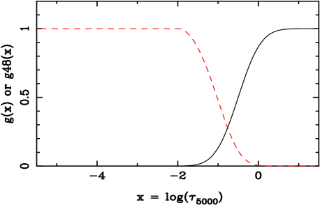
Figure 1: Stratification functions $g(x)$ (solid) and $g_{48}(x)$ (dashed), where $x=\tau_{5000}$. Relevant parameters for the plots are in Tab 3 for $\lambda$8542. Note the minimum of $g(x)$ is not zero, but determined by the parameter $b$. Both $b$ and $g_{48}(x)$ are set to zero for values of $x$ smaller than $10^{-8}$.

Fig. 1 shows a case with the heavy isotope is effectively restricted to layers above $\log(\tau_{5000})$ ca. $-$0.8.

The simplex fits tend to push the centroid of the cloud very high in the model. This tendency had already been noted by Ryabchikova (2005). Additional study of this problem requires a hyperextended atmosphere including non-LTE, which we leave for future work.

3.2 Column densities

In a stratified atmosphere there is no single ${\rm Ca}/N_{\rm tot}$ ratio. As a substitute one may consider integral column densities, for some “equivalent” column length, $H$. We adopt the following, somewhat arbitrary definition.

$$<N_{\rm Ca}H>=\int_{\tau_{\lambda}({\rm min})}^{\tau_{\lambda({\rm max})}}N_{\rm Ca}\exp(-1.5\cdot\tau_{\lambda})\frac{d\tau_{\lambda}}{\kappa_{\lambda}}.$$ (4)

The integrals are taken from the smallest optical depth of our models to the largest, or from $\log(\tau_{5000}=-5.4$ to 1.4.

The $N_{\rm Ca}$-values are calculated with the help of the model atmosphere, and the relevant stratification profile, $g(x)$ or $g_{48}(x)$. With this definition, we can show that very different column densities of ⁴⁸Ca arise in the models with and without isotopic stratification.

A related column density is that of all massive particles. In an obvious notation,

$$<N_{\rm tot}H>=\int_{\tau_{\lambda}({\rm min})}^{\tau_{\lambda({\rm max})}}\frac{P_{g}-P_{e}}{kT}\exp(-1.5\cdot\tau_{\lambda})\frac{d\tau_{\lambda}}{\kappa_{\lambda}}.$$ (5)

From these relations, we may make rough intercomparisons of elemental abundances in stratified and unstratified atmospheres.

3.3 Variable log($gf$)’s

In order to allow for variable relative abundances of individual calcium isotopes, we often adjusted the log($gf$) values for the IRT lines independently. Since the line absorption coefficient involves the product of the abundance and oscillator strength, increasing the $f$- or $gf$-value for a given line is equivalent to increasing the abundance for that line. The elemental and atomic data input to the calculation includes a provisional (note the prime) ratio ${\rm Ca^{\prime}}/N_{\rm tot}$, where $N_{\rm tot}=(P_{g}-P_{e})/(kT)$, (massive particles). When a good line fit is achieved, the provisional ${\rm Ca^{\prime}}/N_{\rm tot}$ is the optimum abundance ratio for that particular line, provided the assumed $gf$-value is also the adopted one. If the $gf$-value differs from that adopted, the abundance that corresponds to a line fit must be modified. Logarithmically,

$$\log({\rm Ca}/N_{\rm tot})_{\rm adopted}=\log({\rm Ca^{\prime}}/N_{\rm tot})_{\rm provisional}$$ (6)

$$+\log(gf)_{\rm used}-\log(gf)_{\rm adopted}$$

In this work we have only assumed the presence of ⁴⁰Ca and ⁴⁸Ca. In some cases, better fits to the observations could have been obtained by including intermediate isotopes, but this has not been done for the present study.

For reference, Tab 1 lists values of log($gf$) from VALD, Meléndez, Bautista, and Badnell (2007, MBB), and Brage et al. (1993, Tab. IV, Col. 3). Convenience motivated our adoption of VALD values, although they are probably less accurate than those of MBB or Brage et al.

Table 1: Recent log($gf$)-values for Ca ii IRT

$\lambda$ [Å]	VALD	Brage et al.	MBB
8498	$-$1.416	$-$1.369	$-$1.366
8542	$-$0.463	$-$0.410	$-$0.412
8662	$-$0.723	$-$0.679	$-$0.675

4 The observational basis for separation of ⁴⁰Ca, ⁴⁸Ca, and perhaps other Ca isotopes

Most of the relevant observational material for isotopic stratification of heavy calcium has been obtained with the UV-Visual Echelle Spectrograph (UVES) at UT2 of the VLT. The instrument and spectra have been described elsewhere (cf. Castelli and Hubrig 2004). Observers may start from the same raw observations, and get spectra that can be significantly different because of the way the material is processed. This seems to be critically true in the region of the Ca ii IRT, and is illustrated in Fig. 2.

Epochs of the spectra illustrated here are given in the figure captions. Many were obtained in August of 2008, and reduced especially for the present study by FG. The remainder were reduced with pipeline programs current for their epoch.

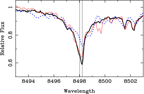
Figure 2: Three reductions of the line $\lambda$8498 of the IRT. All are based on UVES spectra taken on 8 October 2001 of 10 Aql. The vertical lines are at the positions for ⁴⁰Ca (8498.02), and ⁴⁸Ca (8498.22). In order of increasing depth at the latter wavelength, the reductions were made (1) for the ESO archive,
http://archive.eso.org/eso/eso_archive_adp.html UVES Pipeline 3.9.0 (dotted: blue in online version, gray in b/w), (2) for SH in 2006 with UVES Pipeline 2.9.0 and mildly Fourier filtered (thin solid line: red online version, darker gray in b/w), and (3) reduced by FG using IRAF in 2008 (thick: black). Neither (1) nor (3) were Fourier filtered, but all three spectra were rectified as described in Paper III §3.

A relatively small number of stars are suitable for the study of isotopic separation in calcium. First, the large isotopic shifts occur only for the IRT lines. Second, a very small fraction of CP stars show the largest shifts, as may be seen in Figs. 1 and 2 of Paper II. Tab. 2 lists the CP stars with the largest averaged shifts from Paper II. For these stars, the average measured shift of $\lambda\lambda$8498 and 8662 (as well as 8542, when available) is $\geq 0.15$ Å. The seven roAp stars were all included in the study by RKB. Note that HgMn stars are among those with the largest shifts.

4.1 Wavelengths, isotopes, and stratification models

The plots in Papers I and II show unequivocally that the wavelength shifts of all three lines of the IRT are highly correlated. However, the shifts are significantly different in the spectra of (magnetic) CP2 stars (Preston 1974). Measurements of published and recently obtained spectra show that shifts for the $\lambda$8662 are 0.06 Å  larger on the average, than for $\lambda$8498. Average shifts for $\lambda$8542 are similar to those for $\lambda$8498, though in important individual cases (10 Aql, $\gamma$ Equ), the shifts increase from the shortest to the longest wavelength line.

We estimated (Paper II) that any individual wavelength measurement might be uncertain by up to 0.05 Å. These uncertainties could be due to a variety of causes, such as proximity to order gaps, the asymmetry of the line profiles, or to blends. Whatever their cause, shifts of the order of 0.06 Å  are easily measurable, and readily detected in our figures.

At present, we admit that significant differences in the wavelength shifts of IRT lines exist in individual spectra. Their cause has not yet been resolved.

Table 2: CP stars with large IRT wavelength shifts

HD Number	Other	Type	Average Shift
	designation
24712	HR 1217	roAp	0.16
65949		mercury	0.15
101065	Przybylski’s	roAp	0.20
122970		roAp	0.16
133792	HR 5623	roAp	0.18
134214		roAp	0.18
175640	HR 7143	HgMn	0.20
176232	10 Aql	roAp	0.18
178065	HR 7245	HgMn	0.16
217522		roAp	0.20

4.2 Isotopic stratification: different core and wing shifts

Traditional detections of isotopic mixtures or anomalies in stellar atmospheres have been based primarily on wavelength shifts. RKB present plots showing that the mean wavelengths of the $wings$ and cores of IRT lines show different shifts.

These findings are illustrated in their figures 6 and 7, which include four of the stars of Tab. 2. Their Figure 6 is of the $\lambda$8498-line of the sharp-lined spectrum of 10 Aql; figure 6b shows that a calculation assuming a 50-50% mix of ⁴⁰Ca and ⁴⁶Ca+⁴⁸Ca have a wing that is deeper than the observed red wing. The core has a minimum at 8498.20 Å, which would correspond to pure ⁴⁸Ca. They conclude the heavy isotope(s) dominate only in the uppermost layers.

These workers note the difficulty in establishing an accurate observational profile in Section 2 of their paper. We entirely concur (cf. Fig. 2). Their procedure replaces a poor, observed P16 profile by a theoretical one. However, in order to remove the flawed profile, it is necessary to disentangle it from the Ca ii line, and this is not straightforward. One can see this from Fig. 3, which shows the unrectified profile of a single order for 10 Aql, as reduced by FG.

Figure 3: Single order UVES spectrum (8 October 2001) of 10 Aql near $\lambda$8498. The dashed line marks the position of P17. The thick vertical line (actually two virtually unresolved lines) marks the wavelengths of ⁴⁰Ca and ⁴⁸Ca. The centroid of P16 is shown by the vertical line furthest to the right, near a blend of two Si I lines.

We first discuss cases where the evidence for isotopic stratification is strong, and then turn to stars for which the indication of such separation is marginal or absent.

5 HR 1217 (HD 24712)

HR 1217 is the best case that we have examined for isotopic separation. RKB’s Figure 7 shows observational and calculated fits for the intermediate-strength line, $\lambda$8662 as well as $\lambda$8498. Their best fit is shown to be the one with high layers dominated by heavy calcium–isotopic stratification. In Paper II, we reported shifts of 0.17 and 0.15 (respectively) for these two line cores. Our measurements were from a UVESPOP archive spectrum (Bagnulo, et al. 2003), not from the same instrument as used by RKB.

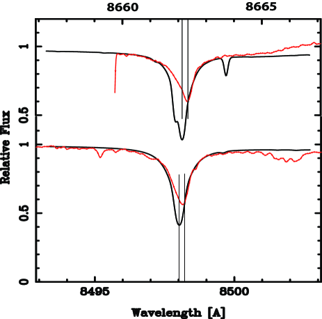
Figure 4: Calculated (black) and observed spectra (gray with dots, red in online version) of IRT lines $\lambda$8662 (above), and 8498 (below) in HR 1217. The UVES spectrum (14 March 2001) is from the UVESPOP archive. The calculations are intended only to show the match of the line wings with an assumption of pure ⁴⁰Ca. The two vertical lines mark the rest wavelengths for ⁴⁰Ca (left) and ⁴⁸Ca (right). The observed red wing of $\lambda$8662 is strongly affected by the order break, and we have moved it to vertically. Clearly lines centered at the position of the vertical lines to the right (⁴⁸Ca) would not fit the observed wings.

We confirm from the UVESPOP spectrum that both lines are readily fit with the heavier isotope, ⁴⁸Ca, providing the shifted core. Fig. 4 is based on the UVESPOP spectrum, and shows that the wings of both the $\lambda$8498 and $\lambda$8662 lines agree with a profile calculated with ⁴⁰Ca only.

6 The Ca ii IRT in 10 Aql

The 10 Aql model used below has $T_{\rm eff}=7650$K, $\log(g)=4.0$, and with solar abundances replaced by appropriate averages (e.g. for neutrals and ions) from Ryabchikova, et al. (2000).

New measurements of the wavelengths of the cores of the IRT lines were obtained from UVES spectra obtained on 4 August 2008. We obtained shifts of +0.17, +0.19, and +0.20 Å , for $\lambda\lambda$8498, 8542, and 8662, respectively. The measured shifts reported in Paper II were +0.14, and +0.22Å  for $\lambda\lambda$8498 and 8662. The differences are consistent with our error estimates for measurements of asymmetrical features.

6.1 The $\lambda$8498 line

The $\lambda$8498 line is the weakest of the IRT. Fig. 5 (upper) shows the result of an automatic (simplex) calculation of the $\lambda$8498 region, using the stratification and abundance parameters for $g(x)$ given in the second column of Tab. 3. For the upper and middle plots, we assumed no variation in isotopic abundances with depth. In the deepest layers of the atmosphere, where $g(x)$ is unity, the value log(Ca${}^{\prime}/N_{\rm tot})$ is the relative abundance provided the oscillator strength is the one accepted. If we accept the VALD value, -1.416, then $\rm\log(^{48}Ca/N_{tot})=-3.75$. The abundance for the more common isotope is smaller by 0.04 dex, because a smaller oscillator strength was required to fit the part of the feature dominated by ⁴⁰Ca. Adding the isotopes, we get $-$3.47 for $\rm\log[(^{40}Ca+^{48}Ca)/N_{tot}]$.

The center plot of Fig. 5 results from trial and error (t&e) adjustments of the parameters to get a better fit near the position of the ⁴⁸Ca core at 8498.22 Å. It is arguable whether an improvement has been achieved, but the total calcium in the deeper layers, log[(⁴⁰Ca+⁴⁸Ca)$/N_{\rm tot}]$ = $-$4.07.

The parameters in the 4th column produced the fit shown in the bottom plot of Fig. 5. This was also a trial and error fit, but adjusted from a simplex solution. The automated result pushed the ⁴⁸Ca cloud so high that only a “sliver” of a region remained with the heavy isotope. Under these conditions, we did not believe the column density calculation was realistic. Note that the $d$-parameter of $g(x)$ is quite small, and this requires a relatively high Ca/$N_{\rm tot}$ ratio in the deepest layers.

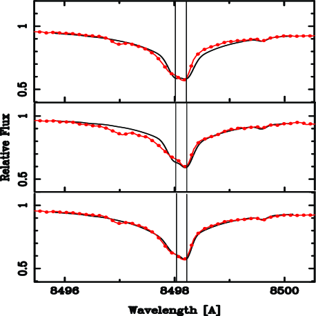
Figure 5: The $\lambda$8498 line in 10 Aql (UVES 4 August 2008). Observed spectra are dark gray (red online) with points, calculations in black. Vertical lines mark the wavelengths for ⁴⁰Ca and ⁴⁸Ca. The upper and middle plots are for a uniform isotopic mix through atmosphere, but elemental stratification. Lower plot assumes isotopic and elemental stratification. Relevant parameters for the fit are in Tab 3.

Table 3: Parameters for 10 Aql fits with (iso-strat) and without (uniform) isotopic stratification. The trial and error (t&e) solution was also made with a uniform isotopic ratio. Abundances are in the rows labeled log(Ca${}^{\prime}/N_{\rm tot})$. These values are multiplied by $g(x)$ or $g_{48}(x)$ respectively in the profile calculation.

	$\lambda$8498			$\lambda$8542
Param.	uniform	t&e	iso-strat	uniform	iso-strat
$a$	4.28	4.0	2.23	4.289	2.0
$\log(b)$	$-$4.72	$-$4.19	$-6.00$	$-$5.133	$-$6.30
$d$	0.4376	0.4	0.110	0.1936	0.0
log(Ca${}^{\prime}/N_{\rm tot})$	$-$3.75	$-$4.19	$-$3.25	$-$3.03	$-$3.30
$\log(gf_{40})$	$-$1.458	$-$1.90	$-$1.416	$-$1.362	$-$0.463
$\log(gf_{48})$	$-$1.416	$-$1.416	$-$5.67	$-$0.463	$-$4.800
$a^{\prime}$			0.949		0.5
$d^{\prime}$			5.00		5.0
$q$			0.185		0.2

There is no question that the fit for $\lambda$8498 is better with the model that assumes isotopic stratification, as claimed by RKB. We shall make an overall assessment after the two stronger IRT lines, and the Ca ii K-line have been discussed.

6.2 The $\lambda$8542 line

Neither of the stronger IRT lines were examined in RKB’s study. The $\lambda$8542 line is the strongest, and was generally unavailable on UVES spectra prior to November 2004. The intrinsic strength of $\lambda$8542 is nearly 9 times greater than that of $\lambda$8498. One therefore expects to see better-developed wings. This should give an increased chance of detecting a wavelength shift—between core and wings—if the core is primarily due to the heavy isotope while the wings are formed deep, where the light isotope dominates.

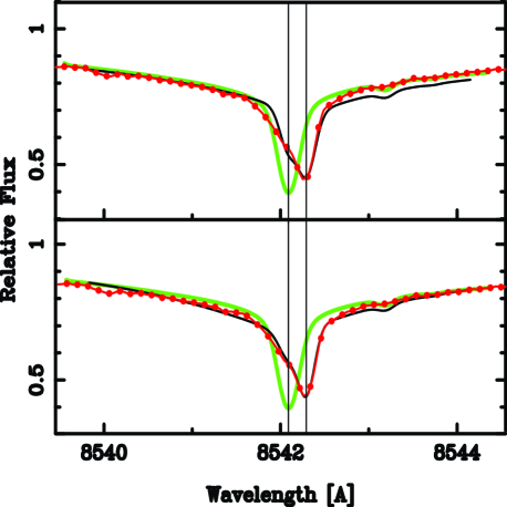
Figure 6: The $\lambda$8542 line in 10 Aql (UVES 4 August 2008). The upper figure: elemental stratification; lower figure: elemental and isotopic stratification. Coding as in Fig. 5. The thick gray line (green in online version) is for a profile with pure ⁴⁰Ca; contrast the behavior of the wings for the profiles. Relevant parameters for the fit are in Tab 3.

The upper part of Fig. 6 shows an automatic (simplex) fit (black) to the observed profile, assuming only elemental stratification. The constant ⁴⁸Ca/⁴⁰Ca ratio is about 6 to 1. Note the greater strength of the calculated red wing, and compare the wing with the observed (dark gray with dots) and profile for pure ⁴⁰Ca (thick lighter gray). This behavior was noted by Ryabchikova and her coworkers (e.g. RKB) as an indication that the wing was formed by a normal (mostly ⁴⁰Ca) mixture.

The lower calculation (black) assumes the ⁴⁸Ca is in a high cloud, with parameters ($g_{48}(x)$) given in Tab. 3. Trial and error improvements were made after an automatic fit to obtain the profile shown.

If we compare the upper and lower parts of Fig. 6, we see the same general features as shown in Fig. 5 for the weaker line, $\lambda$8498. Without isotopic stratification, one cannot get enough absorption in the violet wing without exceeding the observed minimum at the centroid of the absorption for ⁴⁰Ca (left vertical lines in Figs. 5 and 6. The isotopically stratified model can accomplish this because it reduces the amount of ⁴⁰Ca in the upper atmosphere, where the core of the line is formed.

The parameters for the two lines in Tab. 3 in columns 5 and 6 for the two lines differ somewhat for the stratification ($g(x)$, and $g_{48}(x)$). It difficult to judge how meaningful these differences are. Column densities may be more meaningful. We discuss specific results in §6.4.

6.3 The $\lambda$8662 line

The $\lambda$8662 line (not shown) is intrinsically some 55% as strong as $\lambda$8542. It can be fit with parameters similar to those in Tab. 3 for the other two IRT lines. The fit in the near, violet wing is complicated by a strong Fe I line, at 8661.90 Å. If we adjust the iron abundance, or the appropriate $gf$-value for that feature, a fit using only elemental stratification shows the same general features as the other lines of the IRT. Some absorption is missing in the violet wing, and the red wing is too deep.

For the present, we conclude isotopic stratification is the simplest way to explain the IRT profiles in 10 Aql.

6.4 The Ca ii K-line in 10 Aql; overall column densities

Fig. 7 shows our fit to the Ca ii K-line in 10 Aql including a close up of the fit in the core. Relevant stratification parameters are given in the caption.

Tab. 4 compares the column density of the K-line with those for the IRT.

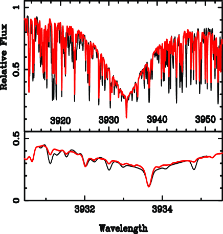
Figure 7: Ca ii K-line fits in 10 Aql. Observation: gray (red online; UVES 8 October 2001), calculation: black. Both plots are centered at $3933.00$ Å  The K-line core ($3933.66$ Å) is therefore noticeably displaced in the lower figure, which shows the inner part of the fit. The stratification parameters are $a=2.2$, $b=3.0\cdot 10^{-6}$, $d=0.1$, and ${\rm Ca}/N_{\rm tot}=2.0\cdot 10^{-4}$.

Table 4: Logarithmic column densities for Ca II lines in 10 Aql.

Isotope$\backslash\lambda$	8498	8542	8662	K-line
Elemental strat. only
48	18.93	19.34	18.85
40	18.90	18.44	18.07
40+48	19.22	19.40	18.92	18.93
Elemental + isotopic strat.
48	14.39	14.46	13.38
40	19.17	19.02	19.29
40+48	19.17	19.02	19.29	18.93

We know of no previous work that has assembled column densities for stratified atmospheres. Thus, we have no basis for judging how well the values for features all arising from Ca ii should agree with one another. The totals for the calculations with elemental stratification only differ by a maximum of 0.48 dex, or a factor of about 3. When isotopic stratification is added, the maximum spread is only slightly less, 0.36 dex or a factor of 2.3.

7 HD 122970

Handler and Paunzen (1999) discovered the roAp nature of HD 122970. It was among the objects studied for elemental and isotopic stratification by Ryabchikova (2005). In Paper I, we gave shifts for $\lambda\lambda$8498 and 8662 of 0.13 and 0.19 Å, respectively. New measurements of all three IRT lines have been made based on spectra obtained in August 2008. They yield the following shifts: 0.15, 0.18, and 0.19 Å  for $\lambda\lambda$8498, 8542, and 8662 respectively. Differences for the measurements in common are 0.02 and 0.00 Å, in good agreement for broad, asymmetrical lines. The tendency to measure the weaker line of the triplet at a smaller shift than the stronger lines is repeated in the remeasurement.

Fig. 8 shows fits of theoretical spectra to the new observations, specially reduced by FG. Our model is based on the parameters of Ryabchikova et al. (2000).

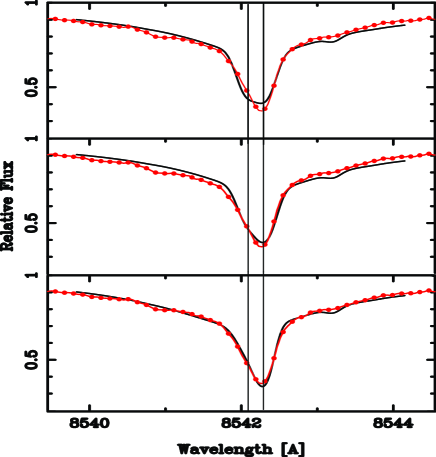
Figure 8: The strongest IRT line, $\lambda$8542 line in HD 122970 without (top, and center) and with (below) isotopic stratification (UVES 3 August 2008). Parameters for the fits are given in Tab. 5. The upper fit was done using the simplex code. The center plot is a trial and error (t&e) fit, starting from the simplex parameters. The lower plot is an unmodified simplex solution (see text).

Table 5: Parameters of $\lambda$8542 fits for HD 122970 with uniform and isotopic stratification. Cols. 2 and 3 refer to the top and center plots of Fig. 8. Col. 4 gives parameters for the lower plot of that figure.

Param.	uniform	uniform	iso-strat
	simplex	t&e	simplex
$a$	6.361	6.300	7.342
$\log(b)$	$-$3.455	-3.301	$-$4.302
$d$	0.562	0.562	0.752
log(Ca/$N_{\rm tot})$	$-$4.947	$-$4.824	$-$5.213
$\log(gf_{40})$	$-$0.708	$-$1.400	$-$0.316
$\log(gf_{48})$	$-$0.460	$-$0.460	$-$0.460
$a^{\prime}$			1.500
$d^{\prime}$			6.488
$q$			0.009

To make a judgement on whether isotopic stratification is indicated, compare the center and lower plots of Fig. 8. Clearly, the lower fit is better. In the middle plot we see the effect pointed out by RKB for the weaker $\lambda$8498 line. The red wing is below the observations, while the violet wing is above. This is explained by the hypothesis of a constant isotopic ratio, which makes too great a contribution to the red wing from the ⁴⁸Ca.

A better fit is shown in the lower part of the figure, where the wings are primarily due to ⁴⁰Ca. The effect is not large, but it is consistent with the effect shown in several papers by Ryabchikova and coworkers, which dealt only with the weaker $\lambda$8498 line. This consistency argues against the possibility that the improved fit is simply due to the additional parameters of the isotopically stratified model.

With isotopic stratification, the simplex calculation puts the maximum of the $g_{48}$ function above the top layer of our model [$\log(\tau_{5000})=-5.4$]. We discussed a similar result in §6.1 for $\lambda$8498 in 10 Aql. The effect was already noted by Ryabchikova (2005). We have noted the need for a study including a hyperextended atmosphere (cf. §8.1), and non-LTE. We find that an equally good fit to the observed profile may be made if we modify the simplex parameters slightly, as we discussed in §6.1. In particular, we used $a^{\prime}=6.0$, $d^{\prime}=5.0$, and $q=0.009$. We get an excellent fit, when we also multiply the $g_{48}(x)$ by 0.01.

With the latter parameters, we find a column density $\rm\log(^{48}CaH)=14.38$, and $\rm\log(^{40}CaH)=18.26$. This relatively very low column density for ⁴⁸Ca should be contrasted with the value that follows from the parameters of the uniform trial and error solution: 18.33. Here, most of the calcium is assumed to be in the heavy isotope, and the total column density is essentially the same as for ⁴⁰Ca with the isotopically stratified model.

The logarithm of the total column density of massive particles is 23.97, so the overall $\rm\log(Ca/N_{tot})$ value is $-$5.64, close to the corresponding solar value, $-$5.65.

8 Gamma Equ

Frequent statements may be found in the literature of CP stars that $\gamma$ Equ and 10 Aql have very similar spectra (cf. Wolff 1983, Ryabchikova, et al. 2000). Probably, the idea goes back to a comment by Bidelman (remark to CRC), whose careful intercomparisons of high resolution spectra of CP stars in the 1960’s were (and are) both highly regarded and well known to those who study the spectra of these stars. Because of its close association with 10 Aql, we include $\gamma$ Equ in the present study, even though the average IRT shifts (0.13 Å) are not quite large enough for it to be included in Tab. 2. Subsequent work has shown that neither the abundances nor the spectra are identical, though the spectra are much more like one another than to many other cool CP stars (cf. $\beta$ CrB, HR 7575).

In Paper II, we fit the $\lambda$8542 line of the IRT. That calculation was made without the current refinements that take Paschen confluence into account (cf. Paper III, Appendix A). The additional continuous opacity from “dissolved” upper levels accounts for a difference in line depth of the order of 0.05 of the continuum, in the line wings. Additionally, the effective oscillator strength of P15 is reduced, because some of the line opacity is now (quasi-) continuous opacity. This could account for the difference of a factor of 4 in the ${\rm Ca^{\prime}}/N_{\rm tot}$ values shown in Tab. 6. While no adjustment to the 10 Aql continuum was made for the specific purpose of fitting the IRT lines, we must admit that the uncertainty in placement of the continuum is of the order of several per cent.

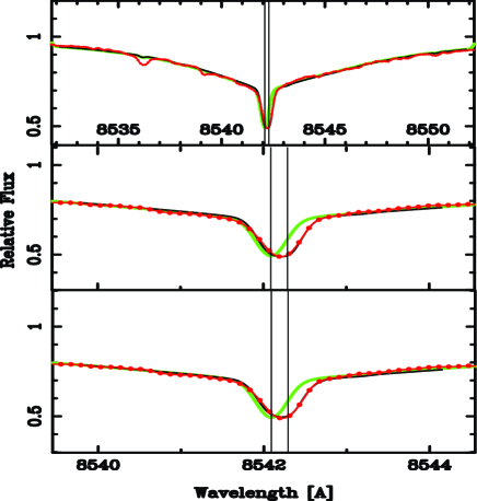
Figure 9: The $\lambda$8542 line in $\gamma$ Equ (UVES spectrum from 18 September 2005). Parameters for $g(x)$ are given in Tab. 6. They apply to the upper and center plots. The lower plot is an automated fit assuming isotopic stratification. The solid black line is the calculation. The observed spectrum is the thin line in dark gray (red in online version). The broad, light gray line (green in online version) shows a fit assuming all of the calcium is ⁴⁰Ca.

Table 6: Parameters of the $\lambda$8542 fit in $\gamma$Equ

$\lambda$8542	Current	Paper II
	work	Fig. 7
Ca’/$N_{\rm tot}$	$1.2\cdot 10^{-4}$	$3.0\cdot 10^{-5}$
$\log(gf)_{40}$	$-$0.46	$-$0.46
$\log(gf)_{48}$	$-$0.36	not used
$a$	6.7	6.7
$b$	$1.5\cdot 10^{-5}$	$10^{-4}$
$d$	0.75	1.0

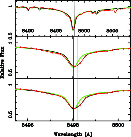
Figure 10: The $\lambda$8498 line in $\gamma$ Equ (UVES spectrum from 18 September 2005). Parameters for $g(x)$, which apply to the upper two plots are: ${\rm Ca^{\prime}}/N_{\rm tot}=7.0\cdot 10^{-4}$, $a=6.7$, $b=2.5\cdot 10^{-6}$, $d=0.30$, $\log(gf)_{40}=-1.12$, $\log(gf)_{48}=-1.32$. The lower plot is an automated fit assuming isotopic stratification. Color coding as in Fig. 9.

Fits to the $\lambda$8498 line are shown in Fig. 10. The stratification parameters and value of ${\rm Ca^{\prime}}/N_{\rm tot}$ are somewhat different from those used for the $\lambda$8542 line. A calculation using the same parameters fits reasonably well in the core and far wings, but is much too strong in the near wings. Optimum parameters are given in the figure.

The third line of the IRT, $\lambda$8662, is well fit by the same stratification parameters as the stronger $\lambda$8542 line, but with ${\rm Ca^{\prime}}/N_{\rm tot}=3.0\cdot 10^{-4}$, and $\log(gf)_{40}=-1.00$, and $\log(gf)_{48}=-0.72$. The differences may not be significant. When we fit the IRT lines in Paper III, we found the same stratification fit the two stronger lines, while the weaker $\lambda$8498 line, required significantly different stratification parameters.

Note the good fits for the red wings in the upper two plots for both Figs. 9 and  10. It does not appear necessary to invoke isotopic stratification to account for the IRT profiles in $\gamma$ Equ.

8.1 The Ca ii K-line in $\gamma$ Equ

In Paper II, we noted (§7.4) that the same parameter set that fit the $\lambda$8542 line also “accounts quite well for the Ca ii K-line profile.” This situation must be reexamined because of the current use of extra opacity from dissolved Paschen lines. We find that slightly modified parameters (cf. Tab. 6, Col. 2) provide a good fit to the K-line: ${\rm Ca}/N_{\rm tot}=9.0\cdot 10^{-5}$, and $d=0.65$. The $a$, and $b$ parameters are the same.

Ryabchikova, et al. (2002, RPK) examined the Ca ii K-line in $\gamma$ Equ in a study that employed a hyperextended atmosphere, to $\log(\tau_{5000})=-10$. Since the center of the K-line saturates in the first depth of our atmosphere [$\log(\tau_{5000})=-5.4$], such an extension would be appropriate. We have experimented with similar models, and find they give essentially the same profiles to the one currently used, provided the temperatures are appropriately adjusted at the shallowest depths. Since such atmospheres are poorly constrained by radiative equilibrium in LTE, we use our standard model here.

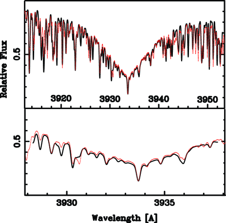
Figure 11: The Ca ii K-line in $\gamma$ Equ (UVES spectrum from 18 September 2005). Parameters for $g(x)$ are: ${\rm Ca}/N_{\rm tot}=9.0\cdot 10^{-5}$, $a=6.7$, $b=1.5\cdot 10^{-5}$, $d=0.65$, $\log(gf)=-0.100$. The central part of the profile is displayed in the lower part of the figure.

Fig. 11 shows a fit to the K-line in $\gamma$ Equ, with a closeup of the core. The parameters are indicated in the caption. An equally good fit may results from parameters, chosen to approximate those shown for calcium in RPK’s Fig. 3. The two stratifications and relevant parameters are given in Fig. 12. The filled stars indicate the stratification profile used by RPK, which deviates at the highest layers from the approximation.

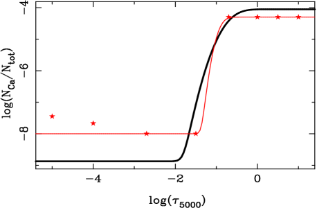
Figure 12: Stratification profiles leading to good fits for Ca ii K-line in $\gamma$ Equ (UVES 18 September 2005). Parameters for the thicker, black curve are given in the caption to Fig. 11. The gray curve (red in online version) is for the function $g(x)$, and used for a fit indistinguishable from that shown in the lower part of Fig 11. The parameters were ${\rm Ca}/N_{\rm tot}=5.0\cdot 10^{-5}$, $\log(gf)=-0.100$, $a=30.0$, $b=2.0\cdot 10^{-4}$, $d=0.9$. See text for the meaning of the filled stars.

9 Stars with weaker calcium lines: Dominant ⁴⁸Ca

9.1 HgMn stars

Several CP stars with large isotopic shifts have rather weak Ca ii and/or IRT lines–certainly relative to HR 1217. RKB do not discuss any of the HgMn stars, which also show varying isotope shifts. Several examples are shown in Fig. 13

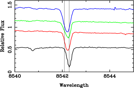
Figure 13: The strongest IRT line, $\lambda$8542 in 4 HgMn stars. Arbitrary vertical displacements of roughly normalized spectra are made for display purposes. The stars, along with the dates of the UVES exposures are from top down: HD 29647 (5 August 2008), HR 1800 (19 September 2005), HR 7245 (18 October 2005), and HR 7143 (20 September 2005). The vertical lines mark the positions of pure ⁴⁰Ca and pure ⁴⁸Ca.

Only HR 7143 (HD 175640) shows the full shift corresponding to ⁴⁸Ca. This star was examined for elemental stratification by Castelli and Hubrig (2004) and Thiam et al. (2008), who reported some evidence for stratification from metallic lines. Elemental stratification is generally accepted for emission lines common in the red and infrared of HgMn and related stars (Sigut 2001). The K-line of Ca ii shows significant wings, and might indicate stratification if it were present. However, Castelli’s web site shows an excellent fit with a non-stratified model: http://wwwuser.oats.ts.astro.it.castelli/hd175640/ p3930-3936.gif

The slope of the “edge” of the HR 1800 profile is steeper on the red side than on the blue. This shape is common among the CP2 stars, as illustrated elsewhere in this paper. Presumably, the more shallow violet slope is caused by an admixture of ⁴⁰Ca. Additional work is needed to investigate the question of isotopic mixtures. The profiles of HD 29647 and HR 7245 could arguably be primarily due to ⁴⁶Ca, which has a shift of 0.16 Å  relative to ⁴⁰Ca. Contributions from lighter as well as heavier isotopes might be required.

One cannot rule out the possibility that the ⁴⁸Ca is in a high, stratified layer. If this were the case, and the low photospheric abundance of calcium were assumed very high, the relative percentage of heavy calcium above the photosphere could be much smaller than it would appear from a naive examination of the profile (see remarks below for the IRT profiles in HR 5623).

Two other HgMn stars in Table A1 of Paper II show large isotopic shifts: HR 6520 (HD 158704) and HR 6759 (HD 165473).

9.2 CP2 stars with weaker IRT lines

Tab. 2 contains CP2 stars with large isotope shifts (ca. 0.2 Å) but moderate or weak IRT lines: HR 5623 (HD 133792), Przybylski’s star (HD 101065), and HD 217522. We discuss them in this order. HR 5623 was the subject of the intensive study of KTR, which introduced the vertical inversion technique. The latter two stars have minor absorption at best that could be attributable to ⁴⁰Ca.

10 HR 5623 (HD 133792)

We devote special attention to HR 5623 because the weakest IRT line, $\lambda$8498 has dominant absorption at the position for ⁴⁸Ca, with a significantly smaller contribution from ⁴⁰Ca. This is shown in Fig. 14. It thus seemed possible that the abundance profile for calcium in HR 5623 approximated that in stars like HR 7143 (HD 175640), where there is no obvious indication of absorption from the lighter isotope at all. Absorption from the stronger line of the $\lambda$8498 blend is roughly double that of the weaker component, presumably due to ⁴⁰Ca, so we might conclude the relative numbers of the isotopes “above the photosphere” was roughly 2 to 1 in favor of ⁴⁸Ca. When absorption from the lighter isotope is entirely missing, there is no way stratification can lead to any conclusion other than ⁴⁸Ca dominates. It might seem that is also the case when the ⁴⁰Ca contribution is relatively weak; stratification would not significantly change the apparent dominance of heavy calcium. However, we shall see that this is not necessarily the case (§10.4).

Figure 14: The $\lambda$8498 line in HR 5623 (UVES spectra 19 March 2006). Vertical lines mark the wavelengths for ⁴⁰Ca and ⁴⁸Ca. While the heavier isotope dominates the absorption, it does not necessarily dominate the number of Ca ions above the photosphere (§3.2, §10.4).

The work by KTR and RKB on this star is based on UVES spectra taken on 26 February 2002. Additional spectra were obtained on 27 January 2005, after reconfiguration of the instrument which move the order gaps away from the IRT lines. IRT shifts from Paper II were +0.18 Å  for both $\lambda\lambda$8498 and 8662. The new measurements yield shifts of +0.19, +0.20, and +0.20 Å  for $\lambda\lambda$8498, 8542, and 8662 respectively.

10.1 Effective temperature and gravity

KTR fixed $T_{\rm eff}=9400$K, and $\log(g)=3.7$ prior to carrying out their vertical inversion calculations. The model parameters were based on Strömgren and H$\beta$ photometry, and the Moon & Dworetsky (1985) calibration as implemented by Rogers (1995, TEMPLOGG). Significantly, they adopted a reddening $E(B-V)=0.09$, which they state “…follows from the reddening maps by Lucke (1978) and high-resolution dust maps by Schlegel, Finkbeiner & Davis (1998).” Additionally, they fit H$\alpha$ and H$\beta$ profiles.

The assumed excess, $E(B-V)=0.09$, follows directly from a standard absorption and reddening law (see Eq. 3.66 of Binney and Merrifield 1998), and the Hipparcos parallax of 5.87 mas. If the color excess is correct it supports the assumed temperature of 9400K.

There is reason to suspect the effective temperature may be several hundred degrees cooler. A code kindly provided to CRC by B. Smalley (private communication), but based on the Moon-Dworetsky (Moon 1984) work gives 8960 or 8900K, depending on whether the reduction is done with Class 5 (A0-A3 III-V), or Class 6 (A3-F0 III-V). The reddenings $E(b-y)$, are $-$0.001 and +0.032 respectively.

We may make an estimate of the reddening from the interstellar sodium lines, with the help of the work of Munari and Zwitter (1997). The equivalent width of the Na D₁ is line difficult to measure precisely, because it is partially blended with the stellar line. We estimate 96 mÅ. From Munari and Zwitter’s Figure 1, one sees that this equivalent width would correspond to $E(B-V)$ values ranging from 0.00 to perhaps 0.10. These authors also provide an empirical fit to the relation between $E(B-V)$ and the equivalent widths of Na D₁ as well as K I $\lambda$7699. We fit a quadratic to the first 5 values of their Table 2, and obtain $E(B-V)=0.026$ from the Na line. The K I feature is arguably present. We estimate an equivalent width of 6.7 mÅ , which would correspond to $E(B-V)=0.020$.

Paunzen, Schnell, and Maitzen (2006) give the excess in the Geneva system as $E(B2-V1)=0.63\cdot E(B-V)$. With this reddening, the Geneva colors (www.unige.ch/sciences/astro/an) give $T_{\rm eff}=8952$K and $\log(g)=3.32$, according to a code kindly supplied by P. North (cf. Kunzli, et al. 1997). This assumes a metallicity ([Fe/H]) of +1, and a reduction grid chosen automatically by the code.

A spectroscopic determination of $T_{\rm eff}$ and log($g$) may be made from the equilibrium of Fe i and ii following the method of Paper III, but using 4 temperatures, 8400, 8900, 9400, and 9900K, and 3 gravities, $\log(g)=3.2$, 3.7, and 4.2. The models assumed abundances taken from KTR when available, otherwise using solar values. A reasonable compromise for the microturbulence is 1 kms^-1. The numerous slopes of $\log({\rm Fe}/N_{\rm tot})$ vs. $\log(W_{\lambda})$ are then sometimes slightly positive, sometimes slightly negative.

Calculations were made using an unstratified model and one stratified model with parameters approximating the profile for iron of KTR, but using a larger jump: $a=20,b=1.0\cdot 10^{-4},d=0.95$. The larger jump was used because KTR found a less than 1 dex jump. We wanted to see the effect of a stronger stratification.

The calculations provide combinations of $T_{\rm eff}$ and $\log(g)$ for which the Fe i and ii give the same abundances. Temperatures with equal abundances from the two stages of ionization are given in Tab 7 for three surface gravities.

Table 7: $T_{\rm eff}$–$\log(g)$ pairs with Fe i and Fe ii in equilibrium. Calculations with and without stratification (“strat,” see text). Corresponding $\rm\log(Fe/N_{tot})$ are given in columns 3 and 5.

$\log(g)$	No Strat	Abund	Strat	Abund
3.2	8914	-3.67	9143	-2.59
3.7	9490	-3.41	9653	-2.34
4.2	9834	-3.21	9916	-2.30

The Geneva photometry and iron equilibrium agree on a low temperature and surface gravity, and no iron stratification. At least some implementations of Strömgren photometry concur. A value of $\log(g)$ as low as 3.2 would be unusual (cf. Hubrig, North, Schöller & Mathys 2007).

Unfortunately, the Balmer lines do not clarify the matter. While KTR support their choice of temperature and gravity by examining H$\alpha$ and H$\beta$, we find these profiles are fit comparably well with $T_{\rm eff}=8900$K, and $\log(g)=3.2$. An example is illustrated in Fig. 15, based on theoretical profiles of Stehlé & Hutcheon (1999). The stellar observations are of low resolution from FORS1 (Appenzeller 1998) which have some advantage over the UVES for broad features. However, we have also examined rectified H$\alpha$ and H$\gamma$ profiles from UVES spectra, and reach similar conclusions.

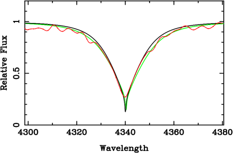
Figure 15: The FORS1 spectrum of H$\gamma$ (dark gray with points) in HR 5623. The light gray plot was made assuming $T_{\rm eff}=9400$K, and $\log(g)=3.7$. The black curve was made using $T_{\rm eff}=8900$K, and $\log(g)=3.2$. The fits are comparable in quality.

10.2 Paschen lines

In principle, the Paschen lines might also resolve the ambiguity in temperature and surface gravity. The situation is hardly better than with the low Balmer lines. Of the three Paschen lines near the IRT, two are significantly influenced by the series convergence. In our calculations P13 ($\lambda$8662) is not strongly affected. We also made calculations for P11 ($\lambda$8862) and P12 ($\lambda$8750). All Paschen profiles used Lemke’s (1997) tables, because the newer Stehlé and Hutcheon calculations do not go to large enough values of $N_{e}$ for high series members. While series convergence is not a problem, photometry and normalization probably is. Calculated profiles for neither of the favored models, gave good fits. We suggest much of the difficulty may lie with the observations, and note that the 2006 UVES spectrum was not re-reduced by FG.

Fig. 16 shows fits of calculated P12 lines to the raw 2006 spectrum, counts vs. wavelength modified only by: shifting the wavelength scale for a radial velocity of 9.3 kms^-1, and dividing the counts by 2746. The fit certainly appears to favor the lower-temperature model, but better observational material is needed. The “raw” P12 profile differed only subtly from the normalized and Fourier filtered version that we typically use. However the small differences were enough that none of the calculated P12 profiles gave a good fit. It seems that our (CRC) best efforts at normalization actually degraded the profile of this and perhaps other broad features.

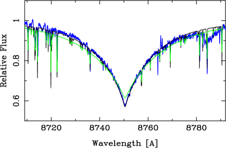
Figure 16: The HR 5623 UVES spectrum (19 March 2006) of P12 (dark gray with points, blue in online version). The light gray curve (green online) was calculated assuming $T_{\rm eff}=9400$K, and $\log(g)=3.7$. The black curve was calculated using $T_{\rm eff}=8900$K, and $\log(g)=3.2$. The overall fit is better for the lower temperature, for both core and wings. No attempt has been made to reconcile the atomic line spectrum with the observations.

10.3 Calcium

We see little basis in the IRT profiles alone for assuming that calcium is isotopically stratified in the atmosphere of HR 5623. This is clear from RKB’s Fig. 8 (uppermost plot), as well as Fig. 17. Indeed, the evidence for any stratification of calcium at all is not strong. This is shown in the lower plot of our figure, as well as Tab. 9. Reasonable fits to all three IRT profiles may be obtained with any one of three contending stratification assumptions: none, elemental, and isotopic.

To show the relative insensitivity of these weak lines to model assumptions, we show the $\lambda$8498 fit to an isotopically stratified model, the $\lambda$8542 fit with elemental, but not isotopic stratification, and the $\lambda$8662 fit with no stratification. Fits of all three lines with any of the three model assumptions closely resemble those shown in the figure.

None of the IRT lines show an indication of displaced wings that would indicate a ⁴⁰Ca-dominated deep photosphere (cf. Fig. 4). Small vertical adjustments of the observed Paschen wings were necessary to achieve the fits shown for the upper plots. We have already noted photometric uncertainties in this region.

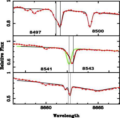
Figure 17: The IRT in HR 5623 (UVES spectra 19 March 2006). The calculated profiles (solid black); observations are dark gray (red online) with dots. The light gray profile for $\lambda$8542 is calculated with ⁴⁰Ca only. There is no indication, as in Fig. 4 that pure (or dominant) ⁴⁰Ca would give a better fit in the red wing. Adjustments (see text) have been made to the Paschen slopes to fit the appropriate Paschen calculations (see text).

The difficulty in extracting a stratification profile for calcium is well illustrated in KTR’s Figure 9. Of the seven lines used, four are only marginally above the level of the noise. Useful information is probably contained in the Ca K-line, but there are difficulties with Ca i $\lambda$4227, and Ca ii $\lambda$3159. The former is badly blended with Cr I, while much of the discrepancy illustrated for the latter may be resolved by taking a cooler model. Additionally, there are continuum problems in the region of this line.

RKB used a different, but partially overlapping, set of Ca i and ii lines from KTR, and obtained somewhat different stratification parameters. We have approximated them with our $g(x)$ function with parameters given in Tab. 8.

Table 8: Abundances and $g(x)$ parameters for approximations to KTR and RKB stratification profiles.

Parameter	KTR	RKB
$a$	6.0	30
$b$	$1.29\cdot 10^{-4}$	$3.16\cdot 10^{-3}$
$d$	0.0	0.6

Only the Ca ii K-line profile approaches the strength needed to see stratification from the line shape alone. Even for the K-line, the case for stratification is marginal. Attempts to derive the stratification from the profile should also consider contributions from an interstellar component.

KTR claimed a Ca overabundance of 1.4 dex in the deep photosphere (see their §6). Assuming a solar $\rm\log(Ca/N_{\rm tot}=-5.73$, KTR’s assumption for this value would be $-$4.32. This should be compared to RKB’s value (see their Tab. 4) $\rm\log(Ca/N_{\rm tot})_{\rm lo}=-5.6$, which is in better agreement with our values (cf. Tab. 9), depending on the assumed model.

Little information is available from Ca i. Most of the lines are very weak or badly blended. Only the resonance line, $\lambda$4227 is of modest strength (ca. 32 mÅ). We calculate abundances for this line, assuming that it is blended with Cr i $\lambda$4226.75, and that the chromium abundance is fixed at $\rm Cr/N_{tot}=1.76\cdot 10^{-4}$. Similarly, we adopted a measured 225 mÅ  for the K-line, and computed abundances from it, including blends with Cr and Fe I, which made only small differences in the resulting abundances. Results for three models, with and without the RKB stratification are given in Tab.9.

Table 9: Logarithmic abundances (log(Ca/$N_{\rm tot}$) from 32 mÅ  $\lambda$4227, and 225 mÅ  K-line. For each model, the upper abundance id for Ca i and the lower for Ca ii Columns marked “diff” are (Ca i $-$ Ca ii). The last three rows give abundances that yield fits to the IRT lines, but only for the 8900K, $\log(g)=3.2$ models. In the case of the stratified model, the abundances refer to the deep photosphere.

$T_{\rm eff}$(K)	$\log(g)$	strat	diff	no strat	diff
9400	3.7	$-5.41$		$-6.49$
		$-6.02$	0.61	$-7.19$	0.70
8900	3.7	$-6.46$		$-7.74$
		$-6.52$	0.06	$-7.50$	$-$0.24
8900	3.2	$-5.92$		$-7.31$
		$-6.32$	0.40	$-7.58$	0.27
$\lambda$(T8900/logg=3.2)		strat		no strat
8498		$-$5.80		$-$8.21
8542		$-$5.54		$-$7.94
8662		$-$5.30		$-$7.82

The best agreement between the K-line and Ca I $\lambda$4227 is for a stratified model with the temperature-log($g$) pair (8900K–3.7). Agreement is poorest at the high temperature. Deep photospheric abundances agree reasonably well among the IRT lines; less well with the K-line and $\lambda$4227.

10.4 Column densities in HR 5623

We calculated column densities for fits to the $\lambda$8498 profile, shown in Figs. 14 and  17. We get a good fit (not shown) using elemental (but not isotopic) stratification, with parameters the same as in column 3 of Tab. 8, but with ${\rm Ca^{\prime}}/N_{\rm tot}$ smaller by a factor of 0.6. This leads to a logarithmic column density for ⁴⁸Ca of 16.51 (cgs) and 16.00 for ⁴⁰Ca.

An equally good fit (Fig. 17) was made with both elemental and isotopic stratification. In this case, the assumed parameters for $g(x)$ were similar, though not identical to those for elemental stratification alone: $a=30$, $d=0.8$, $b=3.16\cdot 10^{-10}$. The ${\rm Ca^{\prime}}/N_{\rm tot}$ value deep in the photosphere was set to $5\cdot 10^{-6}$—this was essentially all ⁴⁰Ca. This $g(x)$ essentially set all of the light isotope to zero abundance for layers higher than $x=-1.5$. The parameters of $g_{48}(x)$ were $a^{\prime}=6$, $d^{\prime}=4$, and $q=3$. These set the abundance of ⁴⁸Ca to zero below $x=0.5$. By $x=-1$, the ${}^{48}{\rm Ca}/N_{\rm tot}$ had reached its maximum value of $4.12\cdot 10^{-9}$.

With isotopic stratification, even though the ⁴⁸Ca feature is stronger, the column density is much lower. We find a logarithmic column density for ⁴⁸Ca of 14.77, while that for ⁴⁰Ca is 17.22, a difference of 2.45 dex.

By column density, the relative fraction of ⁴⁸Ca is smaller, though of the same magnitude, as the terrestrial fraction. This surprising result was noted in §7. It happens because the core regions of the line saturate very high in the atmosphere, and its significance was pointed out by RKB. As far as the core is concerned, the atmosphere below this point is invisible, and to some extent, irrelevant.

The two possible structures examined here surely require very different theoretical scenarios.

11 Przybylski’s Star

The IRT lines in Przybylski’s star appear to have the full shift that would correspond to ⁴⁸Ca. Wavelengths from Paper II, and new measurements from UVES spectra obtained on 1 Jan. 2006 are shown in Tab. 10. It surely seems that ⁴⁸Ca dominates.

Table 10: Independent measurements of the wavelengths of IRT lines in HD 101065. Entries are shifts [Å] from the assumed terrestrial wavelengths at 8498.02, 8542.09, and 8662.14 Å

Spectrum	8498	8542	8662
UVES/2002	0.19		0.19
FEROS/2000	0.16		0.18
UVES/2006	0.21	0.18	0.20

We have not succeeded in finding a stratification profile that will reconcile the deep photospheric abundances from the IRT, the Ca ii K-line, and Ca i lines. Nevertheless, the agreement among these features is somewhat better with a provisional stratification than without one. The parameters are given in Fig. 18 for $\lambda$8662.

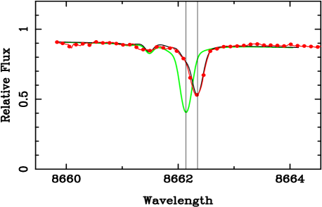
Figure 18: The $\lambda$8662 line in HD 101065 (UVES spectrum 14 January 2006). Vertical adjustments of 3% have been made to achieve a fit to the wings of P13. Calculations are in black, observations dark gray with dots (red online). Stratification parameters are: $a=6.7$, $b=4.0\cdot 10^{-4}$, $d=0.0$. We used log(Ca’/$N_{\rm tot})=-6.20$, and $\xi_{t}=2$ kms^-1. The ratio of ⁴⁸Ca to ⁴⁰Ca is 31.6. The light gray curve was calculated with only ⁴⁰Ca.

We now address the question of whether the heavy calcium dominates the photosphere, or if it occurs in a high cloud above a photosphere with primarily ⁴⁰Ca. We apply the same test as used for HR 1217 and HR 5623, and see if the wings of the IRT lines are better fit with a shifted or unshifted theoretical profiles. We do this for the $\lambda$8662 line (Fig. 18). There is no indication that a pure ⁴⁰Ca composition would yield a better fit to the wings. Compare this situation with that illustrated for HR 1217 (Fig. 4). The failure of pure ⁴⁰Ca to account for the wings of the strongest IRT line, $\lambda$8542, is similar, but the photometry in the P15 wings is not good.

The weakest of the IRT lines shows a slight Zeeman splitting. It is calculated in Fig. 19 assuming pure ⁴⁸Ca, and a transverse field of 2.9 kG. The Zeeman code was described in Paper III. Paschen convergence was not included in this calculation, but the effect is very small, because of the low temperature of HD 101065. The observed profile was lowered by 2% to fit the far P16 wings.

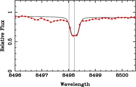
Figure 19: The $\lambda$8498 line in HD 101065 (UVES spectrum 14 January 2006). Vertical adjustments of -2% have been made to achieve a fit to the wings of P16. Calculations are in black, observations dark gray with dots (red online). Stratification parameters are as in Fig. 18. Pure ⁴⁸Ca was assumed. See text for further discussion.

The cause of the broad local minimum on either side of the $\lambda$8498 line is not known. It is unlikely to be due to wings, since the stronger $\lambda$8662 (Fig. 18) and $\lambda$8542 (not shown) do not have extensive wings. The abundance needed for the fit shown was nearly 0.7 dex larger than needed to fit the two stronger IRT lines. It is unclear how meaningful this is, since the function $g(x)$ changes from $5.2\cdot 10^{-4}$ to 0.500 between $\log(\tau_{5000})=-1.0$ and 0.0.

We see little basis in Fig. 19 for assuming any contribution of ⁴⁰Ca to the profile.

12 HD 217522

HD 217522 is a roAp star discussed by Hubrig et al. (2002) as a possible “twin” of Przybylski’s star. Gelbmann (1998) showed that the star is both iron deficient, and at the cool end of the CP star sequence. He argued that this is a general trend among roAp stars.

Measurements on the cores of the IRT lines in HD 217522 show the full 0.20 Å  shift of ⁴⁸Ca. The lines themselves are stronger than in Przybylski’s star but do not show well developed wings. Paper II reported shifts of +0.18 and +0.21 Å, for $\lambda\lambda$8498 and 8662. New measurements of the spectrum obtained on 4 August 2008 yield shifts of +0.20, +0.21, and +0.22 Å, for $\lambda\lambda$8498, 8542, and 8662, respectively.

The IRT can be fit equally well–arguably–with either an isotopic stratification, or a stratification model with a constant ⁴⁸Ca/⁴⁰Ca ratio that is 10-20 to one. We prefer the latter because fewer adjustable parameters are required. Fig. 20 shows a fit of the strongest line, $\lambda$8542. A calculation with pure ⁴⁰Ca is shown in light gray (green online). We obtain quite similar fits for the $\lambda\lambda$8498 and 8662 lines, with similar though not identical stratification and abundance parameters. The plot resembles Fig. 18, where there is no indication that the wings of the stellar feature would be fit better with pure ⁴⁰Ca. Compare Figs. 19 and  20 with Fig. 4.

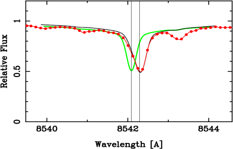
Figure 20: The $\lambda$8542 line in HD 217522 (UVES spectrum 4 August 2008). Stratification parameters ($a=20.0$, $b=1.0\cdot 10^{-4}$, $d=0.1$) and the calcium abundance were chosen to match those used by RKB, ${\rm Ca^{\prime}}/N_{\rm tot}=1.58\cdot 10^{-5}$. The abundance applies to ⁴⁸Ca. A constant abundance ratio of 34.7 was assumed for ⁴⁸Ca/⁴⁰Ca. The light gray curve (green online) was made with pure ⁴⁰Ca.

The same stratification profile and abundance fits the Ca ii K-line reasonably well.

13 Discussion

The profiles of strong lines in CP stars cannot be fit by classical models that assume uniform element to hydrogen ratios throughout the photosphere. We support the assumption of stratification to reconcile the discrepancies with observation, employed by other workers. These attempts are not yet entirely satisfactory because somewhat different stratification models are sometimes needed for lines of the same element or ion.

Ideally, one may determine the stratification parameters directly by comparison with the observations. Thus far workers have chosen a model, and then attributed deviations of observations from calculations to stratification. Possible errors in the assumed model should be folded in to this procedure. Such errors clearly influence the relative strengths of neutrals and ions, as well as lines of a given species with different strengths and excitation. We discussed one relevant example, HR 5623 (HD 133792), where we believe the temperature was significantly overestimated.

We investigated RKB’s bold hypothesis that fractionation of the calcium isotopes could be observed in CP2 stars. We support this claim for HR 1217, using different observational material from their paper. We confirm that good cases for such fractionation can be made for 10 Aql and HD 122970.

One might argue that optimum fits with isotopic stratification are only marginally better than the optimum ones without it. Certainly the additional parameters and model flexibility of the isotopic stratification would be expected to give an improved fit. However, the fits without isotopic stratification show a consistent pattern in a number of stars, including most studied by RKB. The calculated red wings are too strong, indicating too much ⁴⁸Ca in the deeper atmosphere.

RKB wrote (§ 6):

A simple interpretation of the anomaly observed in the Ca ii 8498 Å  line core is to suggest that the heavy isotopes are strongly enhanced and even dominant throughout the atmospheres of some magnetic Ap stars. However, our magnetic spectrum synthesis calculations demonstrate that this hypothesis is incorrect.

The plots in Papers I and II show that the IRT shifts vary from small amounts to nearly the full amounts for ⁴⁸Ca. Only a few stars show the full shifts. Of these, HR 7143, an HgMn star (Castelli and Hubrig 2004), and two roAp stars, HD 101065 and HD 217522 show little or no indication of the lighter isotope. In HR 5623, one may construct a model where ⁴⁸Ca is not dominant, though the most straightforward interpretation of the observations is that it is. In some HgMn stars, the symmetrical profiles may suggest domination by isotopes of intermediate mass.

The overall picture of isotope variations is complex.

14 Acknowledgements

We thank Drs. P. North and B. Smalley for computer codes, and J. R. Fuhr of NIST for advice on oscillator strengths. This research has made use of the SIMBAD database, operated at CDS, Strasbourg, France. We gratefully acknowledge the use of ESO archival data, including the UVESPOP data base. Our calculations have made extensive use of the VALD atomic data base (Kupka, et al. 1999). We appreciate the help of L. Sbordone and P. Bonifacio with implementation of their version of Atlas 9. Thanks are also due to M. Netopil for help during observations in August of 2008.

REFERENCES

Appenzeller, I., Fricke, K., Fürtig, W., et al. 1998, ESO Mess., 94, 1

Babcock, H. W. 1958, ApJ, 128, 228

Babel, J. 1992, A&A, 258, 449

Babel, J. 1994, A&A, 283, 189

Bagnulo, S., Jehin, E., Ledoux, C., et al. 2003, ESO Mess., 114, 10

Binney,J., Merrifield, M. 1998, Galactic Astronomy (Princeton, N. J.: University Press)

Bohlender, D. 2005, in Element Stratification in Stars, 40 Years of Atomic Diffusion, ed. G. Alecian, O. Richard, S. Vauclair, EAS Pub. Ser. 17, 83

Brage, T., Fischer, C. F., Vaeck, N., Godefroid, M., Hibbert, A. 1993, Phys. Scr., 48, 533

Castelli, F., Hubrig, S. 2004, A&A, 425, 263

Cowley, C. R., Hubrig, S. 2005, A&A, 432, L21 (Paper I)

Cowley, C. R., Hubrig, S. 2008, MNRAS, 384, 1588 (Paper III)

Cowley, C. R., Hubrig, S., Castelli, F. 2008, Contr. Astron. Obs. Sk. Pl., 38, 291

Cowley, C. R., Hubrig, S., Kamp, I. 2006, ApJS, 163, 393.

Cowley, C. R., Hubrig, S., Castelli, F., González, F., Wolff, B. 2007, MNRAS, 377, 1579 (Paper II)

Dworetsky, M. M. 2004, in IAU Symp. 224, The A-Star Puzzle, ed. J. Zverko, J. Žižnovský, S. J. Adelman, & W. W. Weiss (Cambridge: Cambridge Univ. Press), p. 499.

Gelbmann, M. J., Cont. Astron. Obs. Ska. Pl., 27, 280

Handler, G., Paunzen, E. 1999, A&AS, 135, 57

Hubrig, S., Cowley, C. R., Bagnulo, S., Mathys, G., Ritter, A., Wahlgren, G. M. 2002, in Exotic Stars as Challenges to Evolution, ASP Conf. Ser., 279, ed. C. A. Tout & W. Van Hamme, p. 365

Hubrig, S., North, P., Schöller, M., Mathys, G. 2007, AN, 328, 475

IMSL (R) Fortran 90 MP Library 3.0, ©visual Numerics, Inc., 1998

Kochukhov, O. 2007, in Physics of Magnetic Stars, eds. I. I. Romanyuk & D. O. Kudryavtsev, 109

Kochukhov, O., Tsymbal, V., Ryabchikova, T., Makaganyk, V., Bagnulo, S. 2006, A&A, 460, 831 (KTR)

Kunzli, M., North, P., Kurucz, R. L., Nicolet, B. 1997, A&AS, 122, 51

Kupka, F., Piskunov, N. E., Ryabchikova, T. A., Stempels, H. C., Weiss, W. W. 1999, A&AS, 138, 119

LeBlanc, F., Monin, D. 2004, in IAU Symp. 224, The A-Star Puzzle, ed. J. Zverko, J. Žižnovský, S. J. Adelman & W. W. Weiss (Cambridge: Cambridge Univ. Press), p. 193

Lemke, M. 1997, A&AS, 122, 285

Lucke, P. B. 1978, A&A, 64, 367

Meléndez, M., Bautista, M. A., Badnell, N. R. 2007, A&A, 469, 1203

Michaud, G. 1970, Ap J, 160, 641

Moon, T. T. 1984, Comm. Univ. London Obs., No. 78

Moon, T. T., Dworetsky, M. M. 1985, MNRAS, 217, 305

Munari, U., Zwitter, T. 1997, A&A, 318, 269

Nesvacil, N., Weiss, W. W., Kochukhov, O. 2008, Cont. Astron. Obs. Ska. Pl., 38, 329

Nörtershäuser, W., Blaum, K., Icker, P., et al. 1998, Eur. Phys. J. D, 2, 33

Paunzen, E., Schnell, A., Maitzen, H. M. 2006, A&A, 458, 293

Preston, G. W. 1974, ARAA, 12, 257

Proffitt, C. R., Brage, T., Leckrone, D. S., Wahlgren, G. M., et al. 1999, ApJ, 512, 942

Rogers, N. Y. 1995, Comm in Asteroseismology, 78

Ryabchikova, T. 2008, Cont. Astron. Obs. Sk. Pl., 38, 257

Ryabchikova, T. 2005, in Element Stratification in Stars, 40 Years of Atomic Diffusion, ed. G. Alecian, O. Richard, S. Vauclair, EAS Pub. Ser. 17, 253

Ryabchikova, T., Kochukhov, O., Bagnulo, S. 2008, A&A, 480, 811 (RKB)

Ryabchikova, T., Leone, F., Kochukhov, O. 2005, A&A, 438, 973

Ryabchikova, T., Savanov, I. S., Hatzes, A. P., Weiss, W. W., Handler, G. 2000, A&A, 357, 981

Ryabchikova, T., Piskunov, N., Kochukhov, O., Tsymbal, V., Mittermayer, P., Weiss, W. W. 2002, A&A, 384, 545 (RPK)

Sbordone, L., Bonifacio, P., Castelli, F., Kurucz, R. L. 2004, Mem. S. A. It. Suppl., 5, 93.

Schlegel, D. J., Finkbeiner, D. P., Davis, M. 1998, ApJ, 500, 525

Sigut, T. A. A. 2001. A&A, 377, L27

Stehlé, C., Hutcheon, R. 1999, A&AS, 140, 93

Thiam, M., Wade, G. A., LeBlanc, F., Khalack, V. R. 2008, Cont. Astron. Obs. Ska. Pl., 38, 461

Wolff, S. C. 1983, The A-Stars: Problems and Perspectives, NASA-SP 463 (see p. 37).

Woolf, V., Lambert, D. L. 1999, ApJ, 521, 414