The positivity and other properties of the matrix of capacitance: physical and mathematical implications

Abstract

We prove that the matrix of capacitance in electrostatics is a positive-singular matrix with a non-degenerate null eigenvalue. We explore the physical implications of this fact, and study the physical meaning of the eigenvalue problem for such a matrix. Many properties are easily visualized by constructing a “potential space” isomorphic to the euclidean space. The problem of minimizing the internal energy of a system of conductors under constraints is considered, and an equivalent capacitance for an arbitrary number of conductors is obtained. Moreover, some properties of systems of conductors in successive embedding are examined. Finally, we discuss some issues concerning the gauge invariance of the formulation.

Keywords: Capacitance, electrostatics, positive matrices, eigenvalue problem, boundary conditions.

PACS: 41.20.Cv, 02.10.Yn, 01.40.Fk, 01.40.gb, 02.30.Tb

1 Introduction

The concept of capacitance and the matrix of capacitance have been studied from several points of view [1]-[15]. On the other hand, the theory of positive matrices and operators is extensively used in branches of Physics such as the mechanics of rigid body motion, quantum mechanics [21, 22], and other more advanced topics [16]-[20]. Nevertheless, the employment of the theory of matrices and operators to study the matrix of capacitance is rather poor [23]-[26]. In particular, no physical meaning is usually given to the eigenvalue problem of the matrix of capacitance. The main topic of this paper is the proof of the fact that the matrix of capacitance is a positive matrix, as well as the mathematical and physical consequences derived from such a fact. The theory of positive matrices and operators permits on one hand to derive some well-known properties of the matrix of capacitance from another point of view, that enlighten the physical meaning of such properties. On the other hand, it allows us to prove new mathematical properties of the matrix of capacitance that lead to an enhancement of our theoretical understanding, but also to new interesting applications.

The paper is distributed as follows: section 2 defines the electrostatic system of conductors that we intend to study, and establishes the notation and properties necessary for our subsequent developments. In Sec. 3 along with Appendix A, the main goal is to prove the positivity of the matrix of capacitance. Sec. 4 discusses some subtleties with respect to the gauge invariance of the formulation. Section 5 along with appendix B explores the physical implications of the positivity of the matrix of capacitance. This is done by constructing a “space of potentials” with inner product in which the matrix of capacitance represents an hermitian positive operator. Section 6 studies the problem of minimization of the internal energy for a system of conductors with constraints, and an equivalent capacitance is defined for a system with arbitrary number of conductors. On the other hand, configurations of conductors that are successively embedded deserves special attention because many simplifications are posible, and this is the topic of Sec. 7 and appendix C. Section 8 summarizes our conclusions and appendix D contains suggested problems for readers.

2 Basic Framework

This section summarizes some properties of the matrix of capacitance obtained in Ref. [27]. They are the framework of our developments in the remaining sections. Let us consider a system of $N$ conductors and an equipotential surface that surrounds them, such equipotential surface could be the cavity of an external conductor. The potential on each internal conductor is denoted by $\varphi_{i}$, $i=1,2,\ldots,N$. (see Fig. 1). We define a set of surfaces $S_{i}$ slightly bigger than the surfaces of the conductors and locally parallel to them, $\mathbf{n}_{i}$ is an unit vector normal to the surface $S_{i}$ pointing outward with respect to the conductor. The potential of the equipotential surface is denoted by $\varphi_{N+1}\$and we define a surface $S_{N+1}\$slightly smaller and locally parallel to the surface of the equipotential. The charges on the conductors are denoted by $Q_{i}$ with $i=1,...,N$ and if there is a cavity of an external conductor in the equipotential surface we denote the charge accumulated in such a cavity by $Q_{N+1}$, the unit vector $\mathbf{n}_{N+1}$ points inward with respect to the equipotential surface. Finally, we define the total surface $S_{T}=S_{1}+\ldots+S_{N+1}$ and the volume $V_{S_{T}}$ defined by the surface $S_{T}$ i.e. the volume delimited by the external surface $S_{N+1}$ and the $N$ internal surfaces $S_{i}$.

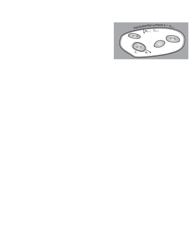
Figure 1: $N$ conductors surrounded by an equipotential surface. The volume $V_{S_{T}}$ is the region in white.

Let us define a set of dimensionless auxiliary functions $f_{i}$ that obey Laplace’s equation in the volumen $V_{S_{T}}$ with the boundary conditions

$$\nabla^{2}f_{j}=0,\text{ \ \ }f_{j}(S_{i})=\delta_{ij},\;\;(i,j=1,\ldots,N+1).$$ (1)

The uniqueness theorem ensures that the solution for each $f_{j}$ is unique in $V_{S_{T}}$. The boundary conditions (1) indicate that the $f_{j}$ functions depend only on the geometry. Since the functions $f_{j}\$acquire constant values on the surfaces $S_{i}$ with $i=1,\ldots,N+1,\$it is clear that $\nabla f_{j}$ is orthogonal to these surfaces. The functions $f_{j}$ have some properties [27]

$$\sum_{j=1}^{N+1}f_{j}=1;\ \nabla f_{j}\left(S_{i}\right)\cdot\mathbf{n}_{i}=\left(1-2\delta_{ij}\right)\left\|\nabla f_{j}\left(S_{i}\right)\right\|;\ 0\leq f_{j}\leq 1$$ (2)

From these auxiliary functions we can construct a matrix that provides a linear relation between the set of charges $Q_{i}$ and the set of potentials $\varphi_{i}$ in the following way

$$C_{ij} \equiv -\varepsilon_{0}\oint_{S_{i}}\nabla f_{j}\cdot\mathbf{n}_{i}\,dS=\varepsilon_{0}\!\int_{V_{S_{T}}}\nabla f_{i}\cdot\nabla f_{j}\,dV$$ (3)

$$Q_{i} = \sum_{j=1}^{N+1}C_{ij}\varphi_{j}$$ (4)

and some properties of the $C_{ij}$ matrix can be derived

$$C_{ij} = C_{ji},\ \ \sum_{j=1}^{N+1}C_{ij}=\sum_{i=1}^{N+1}C_{ij}=0,$$ (5)

$$C_{ii} \geq 0\ \ ,\ \ C_{ij}\leq 0,\ \ \ \ \ \ (i\neq j).$$ (6)

The equations above are valid for $i,j=1,\ldots,N+1$. The expressions below are valid for $i,j=1,\ldots,N$

$$\sum_{i=1}^{N}C_{i,N+1} \leq 0\ \ ,\ \ \sum_{i=1}^{N}C_{ij}\geq 0$$ (7a)

$$|C_{jj}| \geq \sum_{i\neq j}^{N}|C_{ij}|,\ \ C_{ii}C_{jj}\geq C_{ij}^{2}$$ (7b)

$$|C_{N+1,N+1}| = \sum_{i=1}^{N}|C_{i,N+1}|,$$ (7c)

$$|C_{N+1,N+1}| \geq |C_{i,N+1}|$$ (7d)

and expressions for the internal electrostatic energy $$U\$$of the system and of the reciprocity theorem can be obtained

$$U=\frac{1}{2}\sum_{i,j}^{N+1}C_{ij}\varphi_{j}\varphi_{i}=\frac{1}{2}\sum_{i}^{N+1}Q_{i}\varphi_{i};\ \sum_{i=1}^{N+1}Q_{i}\varphi_{i}^{\prime}=\sum_{j=1}^{N+1}Q_{j}^{\prime}\varphi_{j}$$ (8)

where $\left\{Q_{i},\varphi_{i}\right\}$ and $\left\{Q_{i}^{\prime},\varphi_{i}^{\prime}\right\}$ are two sets of charges and potentials over the same configuration of conductors. The $C_{ij}$ elements constitute a real symmetric matrix of dimension $\left(N+1\right)\times\left(N+1\right)$, in which the number of degrees of freedom is $N(N+1)/2$, note that it is the same number of degrees of freedom of a $N\times N$ real symmetric matrix.

For future purposes, we shall call the matrix with elements $C_{ij}\$and with $i,j=1,\ldots,N$ the r-matrix (restricted matrix denoted by $\mathbf{C}$), while the $C_{ij}$ matrix with $i,j=1,\ldots,N+1$ will be called the e-matrix (extended matrix denoted by $\mathbf{C}_{e}$).

3 Discussion of the mathematical properties of the matrix

In this section we establish some additional mathematical properties of the matrix of capacitance. The central fact is that the matrix of capacitance is a positive matrix. Basically, sections 2 and 3 provide the mathematical framework whose physical implications will be explored in the remaining sections.

Equations (1) and (3) tell us that the $C_{ij}$ elements are purely geometrical. In addition, Eqs. (3) and (5) say that the e-matrix is a real symmetric matrix in which the sum of elements of each row and column is null. From Eq. (6) the non-diagonal elements of the e-matrix are non-positive. The volume integral in Eq. (3) shows that the diagonal elements $C_{kk}$ are strictly positive for any well-behaved geometry. In particular, since $C_{N+1,N+1}$ is positive, Eq. (7c) shows that at least one element of the form $C_{i,N+1}$ is different from zero (negative) for $i=1,\ldots,N$; thus rewriting Eq. (5) in the form

$$\ \sum_{j=1}^{N}C_{ij}=-C_{i,N+1}$$ (9)

we see that if $C_{i,N+1}<0\$the sum of the elements of the $i-$row of the r-matrix is positive, if $C_{i,N+1}=0$ such a sum is null. Since at least one of the $C_{i,N+1}$ elements is strictly negative, we conclude that in the r-matrix the sum of elements on each row is non-negative and for at least one row the sum is positive. Because of the symmetry, all statements about rows are valid for columns.

On the other hand, when $V_{S_{T}}$ is a connected region as in Fig. 1, the function $f_{j}$ should change progressively from its value $1$ on conductor $j$ up to the value zero in the conductor $i$ without taking local minima or maxima according to the properties of Laplace’s equation. According with Eq. (2) the factor $\nabla f_{j}\left(S_{i}\right)\cdot\mathbf{n}_{i}$ is positive for $i\neq j$ and from Eq. (3) the non-diagonal $C_{ij}$ factors must be strictly negative for a well-behaved geometry. This discussion is not valid when the volume $V_{S_{T}}$ is non-connected as in Fig. 2, we shall discuss this case in section 7. When $C_{ij}<0$ for $i\neq j$, the discussion below Eq. (9), leads to the fact that the sum of elements in each row of the r-matrix is positive.

In conclusion, for the e-matrix the sum of elements of each row is null. Further, if $V_{S_{T}}$ is a connected region, all matrix elements of the e-matrix are non-null (for a well-behaved geometry), and for the r-matrix the sum of elements of each row is positive. Theorems A and B in Appendix A, show that under these conditions we find: ❶ The e-matrix is a real singular positive matrix, its null eigenvalue is non-degenerate and the other eigenvalues are positive. ❷ The r-matrix is a real positive-definite matrix. Its eigenvalues are all positive. ❸ The null eigenvalue of the e-matrix is associated with $\left(N+1\right)-$dimensional eigenvectors of the form

$$\mathbf{\phi}_{0}^{T}\equiv\left(\varphi_{0},\varphi_{0},...,\varphi_{0}\right)$$ (10)

4 Gauge invariance of the formulation

We shall see that the properties of the matrix of capacitance leads automatically to the gauge invariance of the linear relation between charges and potentials. An outstanding result is that the gauge invariance involving the e-matrix, is closely related with the existence of a null eigenvalue.

We have two possible scenarios here, in the first the equipotential surface is the surface of the cavity of a conductor that encloses the others. In the second, the equipotential surface is just a geometrical place in the vacuum. The uniqueness theorem guarantees the same solution in both cases but only in the interior of the equipotential surface. In the equipotential surface itself we can see that in the first case there is a charge $Q_{N+1}\$accumulated in the cavity, while in the second case there is no charge in such a surface at all. The problem lies in the fact that the electric field is not well-behaved in the surface of the cavity because of the accumulation of surface charge [23]-[26], it is precisely because of this fact that we defined surfaces slightly different from the real surfaces on each conductor (in which $\nabla f_{j}$ are well-defined). So all the observables (charges, potentials, electric fields) are the same in the interior of the equipotential surface for both scenarios, but the surface charge and the electric field differ in both cases when they are evaluated on the equipotential surface itself. Anyway, the internal charges and any other observables not defined on the equipotential surface, are calculated in both scenarios with the same set of $C_{ij}\$coefficients.

From the discussion above, we see that when we have a set of free conductors, the simplest equipotential surface that we can define is the one lying at infinity with zero potential, which is equivalent for most of the purposes to consider a cavity of a grounded external conductor in which all the dimensions of the cavity tend to infinity.

Further, we shall see that the linear relation between charges and potentials in Eq. (4) is gauge invariant by shifting the potential throughout the space as $\varphi^{\prime}\rightarrow\varphi+\varphi_{0}$ with $\varphi_{0}$ being a non-zero constant. This gauge transformation must keep all observables unaltered, in particular the charge $Q_{k}$ on each surface of the conductors. Writing Eq. (4) in matrix form and using Eq. (10) we have

$$\mathbf{Q}^{\prime}=\mathbf{C}_{e}\left(\mathbf{\phi+\phi}_{0}\right)=\mathbf{C}_{e}\mathbf{\phi=Q}$$ (11)

where we used the fact that $\mathbf{\phi}_{0}$ is an eigenvector of $\mathbf{C}_{e}$ with null eigenvalue. This gauge invariance says that there is an infinite number of solutions (sets of potentials) for the linear equations (4) with given values of the charges, this fact is related in turn with the non-invertibility of $\mathbf{C}_{e}$. In other words, gauge invariance is related with the existence of an eigenvector with null eigenvalue which is also equivalent to the non-invertibility. On the other hand, the singularity of a matrix is also related with the linear dependence of the column (or row) vectors that constitute the matrix, this lack of independence in the case of $\mathbf{C}_{e}$ is manifested in the fact that no all charges can be varied independently as can be seen from the expression

$$Q_{int}=-Q_{N+1}$$ (12)

where $Q_{int}$ is the total charge of the internal conductors while $Q_{N+1}$ is the charge accumulated on the surface of the cavity of the external conductor. Further, the linear dependence of the e-matrix can be visualized by observing that it has the same degrees of freedom as the r-matrix. This fact induces us to find expressions involving the r-matrix only. For this, we can rewrite Eq. (4) by following the procedure that leads to Eq. (51)

$$Q_{k}=\sum_{m=1}^{N}C_{km}\left(\varphi_{m}-\varphi_{N+1}\right)\equiv\sum_{m=1}^{N}C_{km}V_{m}$$ (13)

these relations are valid for $k=1,\ldots,N+1$. However, since Eq. (12) shows that $Q_{N+1}$ is not independent, we can restrict them to $k=1,\ldots,N$. Rewriting Eq. (13) in matrix form with this restriction we get

$$\mathbf{Q}=\mathbf{CV};\ \ \mathbf{V}\equiv\left(V_{1},V_{2},...,V_{N}\right),\ \ V_{i}\equiv\varphi_{i}-\varphi_{N+1}$$ (14)

this relation is written in terms of voltages instead of potentials, so it is clearly gauge invariant. Further, the relation is invertible because the r-matrix $\mathbf{C}$ is positive-definite. It worths emphasizing that all expressions obtained from now on in terms of voltages and the r-matrix, are valid only if the voltages are taken with respect to the $\varphi_{N+1}$ potential.

5 Physical implications of the positivity of the matrix

By constructing an appropriate inner product in a “space of potentials”, we shall derive from another point of view some well-known results, such as the reciprocity theorem and the positive nature of the internal energy. As a new result, we give a physical meaning to the eigenvalues and eigenvectors of the capacitance matrix, as well as their relation with the internal energy. Finally, we suggest some ways to determine experimentally the set of eigenvalues and eigenvectors of $\mathbf{C}$, and how these eigenvectors and eigenvalues provide information about $\mathbf{C}$.

To facilitate the derivation and interpretation of the results let us define the following quantities

$$c_{ij}\equiv\frac{1}{k_{0}}C_{ij}\ \ \ ;\ \ \ \Phi_{i}\equiv\frac{1}{k_{0}}Q_{i}$$

where $k_{0}$ is a constant defined such that $c_{ij}$ are dimensionless. From these definitions Eq. (4) could be rewritten in the form

$$\Phi_{i}=\sum_{i=1}^{N+1}c_{ij}\varphi_{j}\ \ ;\ \ \mathbf{\Phi}=\mathbf{c}_{e}\mathbf{\phi}$$ (15)

the dimensionless $c_{ij}$ factors contain the same information as $C_{ij}$. Similarly, $\Phi_{i}$ are quantities with dimension of potential but with the physical information of the charges $Q_{i}$ (it is like a “natural unit” for the charge). The aim of settle the charges and potentials with the same dimension is to interpret Eq. (15) as a linear transformation in the configuration space  $\Phi^{N+1}$ in which each axis has dimensions of potential. This space would be isomorphic to $\mathbb{R}^{N+1}\$if we define an inner product of the form

$$\left(\mathbf{\Phi},\mathbf{\phi}\right)=\mathbf{\Phi}^{\dagger}\mathbf{\phi}=\sum_{i=1}^{N+1}\Phi_{i}\varphi_{i}$$

where we have taken into account that this is a real vector space. The capacitance matrix is hermitian (real and symmetric) with respect to this inner product. Now let us take two sets of charges and potentials $\left\{\mathbf{\Phi},\mathbf{\phi}\right\}$ and $\left\{\mathbf{\Phi}^{\prime},\mathbf{\phi}^{\prime}\right\}$ over the same configuration of conductors. Doing the inner product $\left(\mathbf{\Phi}^{\prime},\mathbf{\phi}\right)$, using Eq. (15) and taking into account the hermiticity of $\mathbf{c}_{e}$, we have

$$\left(\mathbf{\Phi}^{\prime},\mathbf{\phi}\right)=\left(\mathbf{c}_{e}\mathbf{\phi}^{\prime},\mathbf{\phi}\right)=\left(\mathbf{\phi}^{\prime},\mathbf{c}_{e}\mathbf{\phi}\right)=\left(\mathbf{\phi}^{\prime},\mathbf{\Phi}\right)=\left(\mathbf{\Phi},\mathbf{\phi}^{\prime}\right)$$

so that

$$\left(\mathbf{\Phi}^{\prime},\mathbf{\phi}\right)=\left(\mathbf{\Phi},\mathbf{\phi}^{\prime}\right)$$

which is the reciprocity theorem shown in Eq. (8). From this point of view, this theorem is a manifestation of the hermiticity of the e-matrix. Of course, we can define a potential space $\mathbf{\Phi}^{N}$, in which the $N$ internal charges and $N$ voltages form $N-$dimensional vector arrangements and the r-matrix acts as an hermitian operator. In this space the reciprocity theorem acquires the form

$$\left(\mathbf{\Phi}^{\prime},\mathbf{V}\right)=\left(\mathbf{\Phi},\mathbf{V}^{\prime}\right)$$

where in this case $\mathbf{\Phi}^{\prime}$ and$\ \mathbf{\Phi}$ refer to configurations of the internal charges only. Now we shall rewrite the electrostatic internal energy $U\$of the system given by Eq. (8) in our new language

$$u=\frac{1}{2}\left(\mathbf{\phi},\mathbf{c}_{e}\mathbf{\phi}\right)\geq 0\ \ \ ;\ \ u\equiv U/k_{0}$$ (16)

the inequality comes from the positivity of the e-matrix.  This expression is gauge invariant and can be written in terms of the r-matrix and voltages (see appendix B) as follows

$$u=\frac{1}{2}\left(\mathbf{V},\mathbf{cV}\right)\geq 0$$

Because $\mathbf{c}$ is positive-definite, a zero energy is obtained only with $\mathbf{V}=\mathbf{0}$. The only configurations with zero energy are the ones with all potentials equal. Hence, for any geometry of the set of conductors and for any configuration of charges and potentials on them, the external agent that ensembles it, makes a net work on the system. There is no configuration in which the system makes a net work on the external agent. Note that all the analysis above is consistent with the features coming from the equivalent equation

$$u=\frac{1}{2}\int_{V_{S_{T}}}\mathbf{E}^{2}\ dV$$

where $\mathbf{E}$ is the electric field generated by the configuration throughout the volume $V_{S_{T}}$.

Let us interpret the eigenvalue equation of $\mathbf{c}$. It reads

$$\mathbf{cV}^{\left(k\right)}=\lambda_{k}\mathbf{V}^{\left(k\right)}\ \ \Rightarrow\ \ \Phi^{\left(k\right)}=\lambda_{k}\mathbf{V}^{\left(k\right)}$$ (17)

we use superscripts to label a given eigenvector and subscripts to label a given component of a fixed eigenvector. If there is a set $\left\{i\right\}\$of $n$ indices such that all the $\lambda_{i}$’s are identical, this eigenvalue is $n-$fold degenerate. According with Eq. (17), each eigenvector $\mathbf{V}^{\left(k\right)}$ means a configuration of voltages for which each internal charge $\Phi_{i}^{\left(k\right)}\$is related with its corresponding voltage $V_{i}^{\left(k\right)}\$by the same constant of proportionality $\lambda_{k}$. Now, since the eigenvalues are positive, each internal charge $\Phi_{i}^{\left(k\right)}$ and its corresponding voltage $V_{i}^{\left(k\right)}$ have the same sign.

Let us construct a complete orthonormal set of real dimensionless eigenvectors $\mathbf{u}^{\left(k\right)}$ of $\mathbf{c}$ associated with the eigenvalues $\lambda_{k}$. We show in appendix B, Eq. (55) that the internal energy associated with a set of voltages described by the vector $\mathbf{V}\$can be written in terms of those eigenvectors and eigenvalues

$$u=\frac{1}{2}\sum_{n=1}^{N}\lambda_{n}\left|\left(\mathbf{u}^{\left(n\right)},\mathbf{V}\right)\right|^{2}$$ (18)

The set $\left\{\mathbf{u}^{\left(n\right)}\right\}$ defines principal axes in the potential space $\Phi^{N}$,  and $\left(\mathbf{u}^{\left(n\right)},\mathbf{V}\right)$ is the projection of the vector $\mathbf{V}\$along with the principal axis$\ \mathbf{u}^{\left(n\right)}$. If the configuration of voltages in the system is of the form$\ \mathbf{V}^{\left(k\right)}=V_{0}\mathbf{u}^{\left(k\right)}$ (i.e. if the vector $\mathbf{V}$ is parallel to a principal axis) we find

$$u=\frac{1}{2}\lambda_{k}V_{0}^{2}=\frac{1}{2}\lambda_{k}\left\|\mathbf{V}^{\left(k\right)}\right\|^{2}$$ (19)

so the eigenvalue is proportional to the internal energy associated with a set of voltages that forms the corresponding normalized eigenvector of the r-matrix.

Let us suggest now a possible application that illustrates the importance of the eigenvectors and eigenvalues of $\mathbf{c}$. Assume that for a given configuration with $N$ internal conductors, we have calculated the matrix $\mathbf{c}$, as well as $N$ linearly independent eigenvectors $\mathbf{V}^{\left(k\right)}$ and their associated eigenvalues $\lambda_{k}$. We can double-check the correctness of our procedure with the following experiment: Let us settle the experimental arrangement of conductors at the voltages defined by a given eigenvector $\mathbf{V}^{\left(p\right)}$, we then measure the $N$ charges $\Phi_{i}^{\left(p\right)}\$that each internal conductor acquires. Now we calculate the $N$ quotients $\Phi_{i}^{\left(p\right)}/V_{i}^{\left(p\right)}$ where $p$ is fixed. If our calculation of $\mathbf{c}$ was correct, these quotients must be equal (within experimental uncertainties) and must coincide with the eigenvalue $\lambda_{p}$. We can proceed in the same way with each eigenvector. Further, if we measure in each of these configurations the internal energy of the arrangement, we can contrast these experimental values with the ones yielded by Eq. (19).

Though the inverse problem could be difficult in practice, it deserves to say that we can in principle determine eigenvectors and eigenvalues experimentally (adjusting voltages until we find constant quotients between voltages and charges). If we can determine a complete set of eigenvectors and eigenvalues experimentally, the matrix of capacitance can be obtained through a similarity transformation. Defining $\mathbf{X}$ as the matrix of eigenvectors and $\mathbf{\Lambda}$ as the matrix of eigenvalues (we use a $3\times 3$ matrix for illustration)

$$\mathbf{X} \equiv \left(\mathbf{V}^{\left(1\right)}\ \ \mathbf{V}^{\left(2\right)}\ \ \mathbf{V}^{\left(3\right)}\right)\equiv\left(\begin{array}[]{ccc}V_{11}&V_{12}&V_{13}\\ V_{21}&V_{22}&V_{23}\\ V_{31}&V_{32}&V_{33}\end{array}\right)$$ (23)

$$\mathbf{\Lambda} \equiv \left(\begin{array}[]{ccc}\lambda_{1}&0&0\\ 0&\lambda_{2}&0\\ 0&0&\lambda_{3}\end{array}\right)$$ (27)

the $\mathbf{c}$ matrix can be obtained by the relation

$$\mathbf{c}=\mathbf{X\Lambda X}^{-1}$$ (28)

6 Minimization of the internal energy

Problems of minimization of energy under constraints are very useful in Physics. We illustrate by an example a process of minimization of the internal electrostatic energy of a set of conductors under the contraint of constant internal charge. The procedure followed in this section is based on the properties of the $\mathbf{c-}$matrix developed here, and on the Lagrange’s multipliers method, leading naturally to an equivalent capacitance between the external conductor and the set of internal conductors. Such a procedure can be extended to more complex constraints. As an important remark, our example shows that the e-matrix can be useful for practical calculations, despite it does not contain additional degrees of freedom with respect to the r-matrix.

For $N$ internal conductors inside the cavity of an external conductor, let us find the configuration $\mathbf{V}\$of voltages that minimizes the internal energy with the constraint that the total internal charge $Q_{int}\$is a constant $Q_{0}$. Since $Q_{int}=-Q_{N+1}$ and taking into account that Eq. (13) is also valid for $k=N+1$, we have

$$Q_{int}=-\sum_{j=1}^{N}C_{N+1,j}V_{j}=Q_{0}$$ (29)

the function $Z\left(\mathbf{V}\right)$ that defines the constraint is

$$Z\left(\mathbf{V}\right)\equiv-\sum_{j=1}^{N}C_{N+1,j}V_{j}-Q_{0}=0$$ (30)

from the Lagrange’s multipliers method we have

$$\frac{\partial U}{\partial V_{i}}+\beta\frac{\partial Z}{\partial V_{i}}=0\ \ ;\ \ i=1,\ldots,N$$ (31)

where $\beta$ is the multiplier. Writing the internal energy as

$$U=\frac{1}{2}\left(\mathbf{V},\mathbf{CV}\right)=\frac{1}{2}\sum_{k=1}^{N}\sum_{j=1}^{N}V_{k}C_{kj}V_{j}$$ (32)

replacing Eqs. (30, 32) into Eq. (31) and using the symmetry of the matrix, we find

$$\sum_{j=1}^{N}C_{ij}V_{j}=\beta C_{i,N+1}\ \ ;\ \ i=1,\ldots,N$$ (33)

and applying a sum over $i\$on Eq. (33)

$$\sum_{j=1}^{N}V_{j}\sum_{i=1}^{N}C_{ij} = \beta\sum_{i=1}^{N}C_{i,N+1}\ ,$$ (34)

$$-\sum_{j=1}^{N}V_{j}C_{N+1,j} = -\beta C_{N+1,N+1}$$ (35)

where we have used (5). Subtracting Eqs. (35, 29) and solving for $\beta$ we find

$$\beta=-\frac{Q_{0}}{C_{N+1,N+1}}$$ (36)

Eq. (33) can be rewritten as

$$\mathbf{CV}=\beta\mathbf{v}_{c}\ \ ;\ \ \mathbf{v}_{c}^{T}\equiv\left(C_{1,N+1},C_{2,N+1},...,C_{N,N+1}\right)$$ (37)

For a given $\beta$, the solution of Eq. (37) is unique because the r-matrix $\mathbf{C}$ is invertible. It is easy to check that $\mathbf{V}=\left(V_{a},...,V_{a}\right)$, is a solution of Eq. (37), inserting this solution in Eq. (37), we get

$$V_{a}\sum_{j=1}^{N}C_{ij} = \beta C_{i,N+1}\ ,\ i=1,\ldots,N$$

$$-V_{a}C_{i,N+1} = \beta C_{i,N+1}\ ,\ i=1,\ldots,N$$ (38)

where we have used (5). From (38) we have

$$V_{a}=-\beta$$ (39)

Thus, the configuration of $N\$voltages that minimizes the energy with a fixed value of $Q_{int}$, is given by

$$\mathbf{V}^{T}=\left(-\beta,-\beta,...,-\beta\right)$$ (40)

This kind of solution for $\mathbf{V}\$is expected because the configuration of minimal energy is obtained when we connect all the internal conductors among them by conducting wires, this procedure clearly keeps $Q_{int}$ constant and equates internal potentials. Since all potentials of the interior conductors are the same, we can define a single voltage between the external conductor and the internal ones, this voltage is $\left|\beta\right|$. Since $Q_{int}=-Q_{N+1}=Q_{0}$ we can figure out the system as equivalent to a system consisting of two conductors with charges $\pm Q_{0}\$and voltage $\left|\beta\right|$. Thus, we are led naturally to an equivalent capacitance for this system of potentials and charges

$$\left|Q_{0}\right|=C_{eq}\left|\beta\right|\ \ \Rightarrow\ \ C_{eq}=\left|\frac{Q_{0}}{\beta}\right|=C_{N+1,N+1}$$

where we have used Eq. (36). It can be checked that the internal energy $U$ for the configuration described by (40) is

$$U=\frac{1}{2}C_{N+1,N+1}V_{a}^{2}=\frac{1}{2}C_{eq}\beta^{2}$$ (41)

as expected. A brief comment with respect to the e-matrix is in order. This matrix has no additional degrees of freedom with respect to the r-matrix so that we can formally write all results in terms of the elements $C_{ij}$ of the r-matrix. Notwithstanding, the extended elements could be useful for explicit calculations. Assume for instance that for the problem in the present section, we want to calculate the total internal charge for a given voltage of the system, and the equivalent capacitance. These calculations can be done with the following expressions

$$Q_{int} = \sum_{i=1}^{N}Q_{k}=V_{a}\sum_{i=1}^{N}\sum_{j=1}^{N}C_{ij}=C_{eq}V_{a}$$

$$C_{eq} = C_{N+1,N+1}=-\sum_{i=1}^{N}C_{i,N+1}=\sum_{i=1}^{N}\sum_{j=1}^{N}C_{ij}$$

Therefore, in terms of the elements of the r-matrix all the $N(N+1)/2\$coefficients must be evaluated with Eq. (3), to calculate $Q_{int}$ and $C_{eq}$. In contrast, by using the e-matrix, only the $C_{N+1,N+1}\$coefficient should be calculated through Eq. (3) to find such observables. This difference becomes more important as $N$ increases. Similar advantages of using the e-matrix appear in more general contexts (see appendix A of Ref. [27]).

7 The case of a chain of embedded conductors

Let us consider a system of conductors in successive embedding as described in Fig. 2 and in appendix C. We encounter such systems quite often in Physics. We observe that in systems as the one in Fig. 1, the volume $V_{S_{T}}$ consists of a “single piece”, but in successively embedded conductors such a volume consists of “several disjoint pieces” as shown in Fig. 2. The main consequence coming from this difference is the fact that some elements of the matrix of capacitance are null for embedded systems. This fact simplifies considerably the calculation of such a matrix. However, we shall prove that the other properties of the matrix of capacitance remains the same.

Section 3 shows that the e-matrix is singular positive and the r-matrix is positive-definite. The first fact was independent of the connectivity of $V_{S_{T}}$. In contrast, the second fact was derived from the statement that all non-diagonal $C_{ij}$ elements were strictly negative. However, it is shown in appendix C that in the case of a chain of embedded conductors (see Fig. 2), some of the non-diagonal elements $C_{ij}$ are null because the volume $V_{S_{T}}$ is disconnected. Then we should check whether the r-matrix is still positive-definite for the chain of embedded conductors.

Appendix C shows that elements of the form $C_{i,i\pm 1}$ are non-zero in general. Appealing to an argument analogous to the one presented in Sec. 3 we can show that for a well-behaved geometry of our embedded conductors, $C_{ii}>0$ and $C_{i,i\pm 1}<0$, while the remaining elements vanish. With these properties and the fact that the sum of elements of each row of the e-matrix is null, we see that the sum of elements in each row of the r-matrix is null except for the $N-$row, for which the sum is positive. Therefore, the r-matrix of a chain of embedded conductors satisfies the conditions of theorem C in appendix A. Consequently, for a chain of embedded conductors, the r-matrix continues being positive-definite, and the e-matrix is still singular positive. Combining these facts with theorem B of appendix A, we obtain that the null eigenvalue of the e-matrix is non-degenerate. It is again consistent with the fact that the only configuration of null internal energy is the one associated with all conductors at the same potential.

8 Conclusions

We have studied an electrostatic system consisting of a set of $N$ conductors with an equipotential surface that encloses them. The associated matrix of capacitance has dimensions $\left(N+1\right)\times\left(N+1\right)$ (extended or e-matrix) even if the equipotential surface goes to infinity. It is usual in the literature to work with the matrix of dimension $N\times N$ (restricted or r-matrix), this practice is correct only if the voltage of the conductors is taken with respect to the potential of the equipotential surface. We prove that the e-matrix is a real positive and singular matrix, this is consistent with the fact that gauge invariance requires the existence of a null non-degenerate eigenvalue of this matrix. The r-matrix is a real positive-definite matrix so all its eigenvalues are positive.

By constructing a “potential space” with inner product, we can derive some results such as the reciprocity theorem and the non-negativity of the electrostatic internal energy of the system, from another point of view. A given eigenvector $\mathbf{V}^{\left(p\right)}\$of the r-matrix corresponds to a set of voltages $V_{i}^{\left(p\right)}$,  such that if we settle the internal conductors at these voltages, the charges $Q_{i}^{\left(p\right)}$ acquired by each internal conductor $i$,  are such that the quotient $\lambda_{p}=Q_{i}^{\left(p\right)}/V_{i}^{\left(p\right)}\$is the same for all internal conductors and corresponds to the eigenvalue associated with $\mathbf{V}_{i}^{\left(p\right)}$. The positivity of the eigenvalues $\lambda_{p}$ guarantees that each charge $Q_{i}^{\left(p\right)}$ posseses the same sign as the associated voltage $\mathbf{V}_{i}^{\left(p\right)}$. In addition, a given eigenvalue is proportional to the internal energy associated with the set of voltages generated by its corresponding eigenvector. Moreover, a complete set of orthonormal eigenvectors of the r-matrix defines principal axes in the “potential space”. It worths emphasizing that eigenvectors and eigenvalues can be measured experimentally, and provide information about the matrix of capacitance.

The problem of the minimization of the internal energy is studied under the constraint of constant value of the total internal charge. In this case we can define an equivalent capacitance for any number of internal conductors. From this problem, we realized that although the e-matrix has the same degrees of freedom as the r-matrix, such extension could lead to great simplifications of some practical calculations.

Further, systems of successive embedded conductors are analyzed showing that some coefficients of capacitance are null for these systems, allowing an important simplification for practical calculations. This fact is related with connexity properties of the volume in which Laplace’s equation is considered. Moreover, we prove that for these configurations of embedded conductors the e-matrix is still positive singular with a non-degenerate eigenvalue and the r-matrix is positive-definite.

Finally, the properties of the matrix of capacitance shown here, can be useful for either a formal understanding or practical calculations in electromagnetism. It worths observing the similarity in structure between the matrix of capacitance and the inertia tensor.

Appendix A Some special types of matrices

This appendix concerns the study of a special type of matrices. Let define $\Sigma_{k}$ as the sum of the elements on the $k-$row of a given matrix. We shall make the following

Definition: A sp-matrix, is a square real matrix of finite dimension  in which $c_{mk}=c_{km}\leq 0$ for $k\neq m$, and in which $\Sigma_{k}$ is non-negative for all $k$. We denote with a single prime $\left\{k^{\prime}\right\}$ the set of indices for which $\Sigma_{k^{\prime}}>0$ and with double prime $\left\{k^{\prime\prime}\right\}$ the set of indices for which$\ \Sigma_{k^{\prime\prime}}=0$. If no prime is used, either situation could happen.

Theorem A: If $\mathbf{C}$ is a sp-matrix, then $\mathbf{C}$ is a positive matrix with respect to the usual complex inner product. ➊ If $\left\{k^{\prime}\right\}$ is empty, the matrix is singular and vectors of the form $\mathbf{N}_{0}^{T}=\left(n,\ldots,n\right)$ are eigenvectors of $\mathbf{C}$ with null eigenvalue. Further, the null eigenvalue is non-degenerate if all elements of the matrix are non-null. ➋ If $\left\{k^{\prime\prime}\right\}$ is empty, the matrix is positive-definite.

Proof: We should prove that

$$\mathbf{V}^{\dagger}\mathbf{CV}\geq 0$$ (42)

for an arbitrary vector $\mathbf{V}$,  and we should look under what conditions exists at least one non-zero vector $\mathbf{V\ }$for which this bilinear expression is null. Rewriting $\mathbf{V}=\mathbf{N}+i\mathbf{M}$ with $\mathbf{N},\ \mathbf{M}$ being real vector arrangements, and using the symmetry of $\mathbf{C}$, the bilinear form in Eq. (42) becomes$\ \mathbf{N}^{T}\mathbf{CN}+\mathbf{M}^{T}\mathbf{CM}$. Therefore, it suffices to prove the positivity (or non-negativity) of the bilinear form with real vector arrangements. Let $\mathbf{N}$ be a non-zero real vector, the associated bilinear form is

$$\mathbf{N}^{T}\mathbf{CN}=\sum_{k}n_{k}c_{kk}n_{k}+\sum_{k}\sum_{m\neq k}c_{km}~{}n_{k}n_{m}$$

for the remaining of this appendix, we assume that indices labeled with different symbols are strictly different. We rewrite the bilinear form as

$$\mathbf{N}^{T}\mathbf{CN} = \sum_{k}\left\{c_{kk}n_{k}^{2}\right.$$

$$+\frac{1}{2}\sum_{m}c_{km}[n_{k}^{2}+n_{m}^{2}-(n_{k}-n_{m})^{2}]\}$$

$$\mathbf{N}^{T}\mathbf{CN} = \sum_{k}\left\{\left[c_{kk}+\frac{1}{2}\sum_{m}c_{km}\right]n_{k}^{2}+\frac{1}{2}\sum_{m}c_{km}n_{m}^{2}\right\}$$ (43)

$$-\frac{1}{2}\sum_{k}\sum_{m}c_{km}\left(n_{k}-n_{m}\right)^{2}$$

Now, since $\Sigma_{k}=c_{kk}+\sum_{m}c_{km}\geq 0$, we have

$$c_{kk}+\frac{1}{2}\sum_{m}c_{km}\geq-\frac{1}{2}\sum_{m}c_{km}$$ (44)

it is convenient to separate the sets $\left\{k^{\prime}\right\}$ and $\left\{k^{\prime\prime}\right\}$ in Eq. (44)

$$c_{k^{\prime\prime}k^{\prime\prime}}+\frac{1}{2}\sum_{m}c_{k^{\prime\prime}m} = -\frac{1}{2}\sum_{m}c_{k^{\prime\prime}m}$$ (45)

$$c_{k^{\prime}k^{\prime}}+\frac{1}{2}\sum_{m}c_{k^{\prime}m} > -\frac{1}{2}\sum_{m}c_{k^{\prime}m}$$ (46)

we examine first the case in which $\left\{k^{\prime}\right\}$ is empty. In that case there are no equations of the type (46), and all indices accomplish the equation (45). Using (45) in Eq. (43) and the fact that $c_{km}\leq 0$, we find

$$\mathbf{N}^{T}\mathbf{CN} = \sum_{k}\left\{\left[-\frac{1}{2}\sum_{m}c_{km}\right]n_{k}^{2}+\frac{1}{2}\sum_{m}c_{km}n_{m}^{2}\right\}$$

$$+\frac{1}{2}\sum_{k}\sum_{m}\left|c_{km}\right|\left(n_{k}-n_{m}\right)^{2}$$

using the symmetry of the matrix and taking into account that $k,m$ are dumb indices, the first two terms on the right-hand side vanish and we find

$$\mathbf{N}^{T}\mathbf{CN}=\frac{1}{2}\sum_{k}\sum_{m}\left|c_{km}\right|\left(n_{k}-n_{m}\right)^{2}\geq 0$$ (47)

Equation (47) shows that the bilinear form is always non-negative and that $\mathbf{N}^{T}\mathbf{CN}=0$ for non-zero vector arrangements of the form $\mathbf{N}_{0}^{T}\equiv\left(n,n,\ldots,n\right)$. Consequently, the matrix is singular positive. We can check that $\mathbf{N}_{0}$ is an eigenvector of $\mathbf{C}$,  with null eigenvalue. If all elements $c_{km}$ are non-null, Eq. (47) shows that this is the only linearly independent solution, so that the zero eigenvalue is non-degenerate.

Now we examine the case in which $\left\{k^{\prime\prime}\right\}$ is empty, so there are no equations of the type (45), and all indices accomplish the equation (46). Replacing (46) into Eq. (43), using the symmetry of $\mathbf{C}$, the fact that $c_{km}\leq 0$, and that $\mathbf{N}\neq 0\$we find

$$\mathbf{N}^{T}\mathbf{CN}>\frac{1}{2}\sum_{k}\sum_{m}\left|c_{km}\right|\left(n_{k}-n_{m}\right)^{2}\geq 0$$ (48)

and the bilinear form becomes positive if and only if $\mathbf{N}\neq 0$. Hence, the sp-matrix is positive-definite when $\left\{k^{\prime\prime}\right\}$ is empty. QED.

Theorem B: Let $\mathbf{C}$ be a matrix of dimension $\left(N+1\right)\times\left(N+1\right)$, such that $\Sigma_{i}=0$ for all rows. This matrix has eigenvectors of the form $\mathbf{N}_{0}^{T}=\left(n,\ldots,n\right)$ associated with a null eigenvalue. Let $\mathbf{C}_{r}$ be the $N\times N\$submatrix of $\mathbf{C}$ consisting of the elements $C_{ij}$ of $\mathbf{C\ }$with $i,j=1,\ldots,N$. If $\mathbf{C}_{r}$ has no null eigenvalues, the null eigenvalue of $\mathbf{C}$ is non-degenerate.

Proof: The condition $\Sigma_{i}=0$ for $i=1,\ldots,N+1$ gives

$$\sum_{k=1}^{N+1}C_{ik}=0\ \ ;\ \ i=1,\ldots,N+1$$ (49)

Eigenvectors of $\mathbf{C}\$with null eigenvalues must give

$$\sum_{k=1}^{N+1}C_{ik}n_{k}=0\ \ ;\ \ i=1,...,N+1$$ (50)

assuming $n_{k}=n$ for all $k$ and using condition (49), Eq. (50) is satisfied. Thus, $\mathbf{N}_{0}^{T}$ is an eigenvector associated with a null eigenvalue. From the condition (49) we also find

$$\sum_{k=1}^{N+1}C_{ik}n_{k} = \sum_{k=1}^{N}C_{ik}n_{k}+C_{i,N+1}n_{N+1}$$

$$= \sum_{k=1}^{N}C_{ik}n_{k}+\left(-\sum_{k=1}^{N}C_{ik}\right)n_{N+1}$$

$$\sum_{k=1}^{N+1}C_{ik}n_{k} = \sum_{k=1}^{N}C_{ik}\left(n_{k}-n_{N+1}\right);\ i=1,..,N+1$$ (51)

replacing (51) in (50) the latter becomes

$$\sum_{k=1}^{N}C_{ik}\left(n_{k}-n_{N+1}\right)=0\ ;\ \ i=1,...,N+1$$ (52)

in particular Eq. (52) holds for $i=1,...,N$. With this restriction Eq. (52) becomes

$$\mathbf{C}_{r}\mathbf{V}=0\ ;\ \ \mathbf{V}\equiv\left(n_{1}-n_{N+1},n_{2}-n_{N+1},...,n_{N}-n_{N+1}\right)$$ (53)

since $\mathbf{C}_{r}$ has no null eigenvalues, the only solution for Eq. (53) is $\mathbf{V}=\mathbf{0}$. Hence the only type of solutions for $\mathbf{N}$ are of the form $\mathbf{N}=\left(n_{N+1},n_{N+1},...,n_{N+1}\right)$ which are all linearly dependent. Hence, the null eigenvalue is non-degenerate. It is immediate that these solutions satisfy Eq. (52) for $i=N+1$ as well. Note that $\mathbf{C}$ is not necessarily symmetric or real. QED.

Theorem C: Let $\mathbf{C\ }$be  a$\ N\times N\$sp-matrix such that $\left\{k^{\prime\prime}\right\}=\left\{1,2,\ldots,N-1\right\}\$and the terms

$$c_{i,i+1}=c_{i+1,i}\ \ ,\ c_{i,i-1}=c_{i-1,i}\ \ ;\ \ i=2,...,N-1$$

are non-zero, while the remaining non-diagonal terms vanish. Then $\mathbf{C}$ is positive-definite.

Proof: Assume $\mathbf{C}$ as singular and arrive to a contradiction. Replacing Eqs. (45, 46) in Eq. (43) we obtain

$$\mathbf{N}^{T}\mathbf{CN} \geq \sum_{k}\left\{\left[-\frac{1}{2}\sum_{m}c_{km}\right]n_{k}^{2}+\frac{1}{2}\sum_{m}c_{km}n_{m}^{2}\right\}$$

$$-\frac{1}{2}\sum_{k}\sum_{m}c_{km}\left(n_{k}-n_{m}\right)^{2}$$

such a replacement also shows that the equality holds if $n_{N}=0$, while the strict inequality holds if $n_{N}\neq 0$. Using the symmetry of the matrix and the fact that $c_{km}\leq 0$ we have

$$\mathbf{N}^{T}\mathbf{CN}\geq\frac{1}{2}\sum_{k}\sum_{m}\left|c_{km}\right|\left(n_{k}-n_{m}\right)^{2}$$

Since $\mathbf{C}$ is singular, a non-trivial solution must exist for the bilinear form to be null. For this, the equality must hold in this relation, therefore $n_{N}=0$. The term on the right written in terms of the non-zero elements of the matrix yields

$$\mathbf{N}^{T}\mathbf{CN} = \frac{\left|c_{12}\right|}{2}\left(n_{1}-n_{2}\right)^{2}+\sum_{k=2}^{N-1}\frac{\left|c_{k,k+1}\right|}{2}\left(n_{k}-n_{k+1}\right)^{2}$$

$$+\sum_{k=2}^{N-1}\frac{\left|c_{k,k-1}\right|}{2}\left(n_{k}-n_{k-1}\right)^{2}+\frac{\left|c_{N,N-1}\right|}{2}n_{N-1}^{2}$$

for this expression to be zero each term in these sums must be zero. Since all matrix elements involved in this expression are non-zero, the last sum says that $n_{N-1}=0$, while the other sums say that $n_{1}=n_{2}=...=n_{N-1}$. Since $n_{N}$ was already zero, it shows that the only solution is the trivial one, contradicting the singularity of the matrix. QED.

Appendix B Some properties of the internal energy

The equation (16) for the internal energy $u\$in “natural units” can be written in terms of voltages instead of potentials with the r-matrix. By using the fact that $\mathbf{\phi}_{0}$ is an eigenvector of $\mathbf{c}_{e}$ with null eigenvalue, and the hemiticity of $\mathbf{c}_{e}$, Eq. (16) becomes

$$2u = \left(\mathbf{\phi},\mathbf{c}_{e}\left(\mathbf{\phi-\phi}_{0}\right)\right)=\left(\mathbf{c}_{e}\mathbf{\phi},\left(\mathbf{\phi-\phi}_{0}\right)\right)$$

$$2u = \left(\mathbf{c}_{e}\left(\mathbf{\phi-\phi}_{0}\right),\left(\mathbf{\phi-\phi}_{0}\right)\right)=\left(\mathbf{\phi-\phi}_{0},\mathbf{c}_{e}\left(\mathbf{\phi-\phi}_{0}\right)\right)$$

defining a vector arrangement of $N+1\$voltages $\mathbf{V}_{e}$ we find

$$2u=\left(\mathbf{V}_{e},\mathbf{c}_{e}\mathbf{V}_{e}\right);\ \ \mathbf{V}_{e}^{T}\equiv\left(V_{1},...,V_{N},V_{N+1}\right),\ \ V_{i}\equiv\varphi_{i}-\varphi_{0}$$

writing this bilinear form explicitly and expanding the sums we find

$$u = \frac{1}{2}\sum_{i=1}^{N+1}\sum_{j=1}^{N+1}c_{ij}V_{i}V_{j}$$

$$= \frac{1}{2}\sum_{i=1}^{N}\sum_{j=1}^{N}c_{ij}V_{i}V_{j}+V_{N+1}K_{N+1}$$

$$K_{N+1} \equiv \sum_{i=1}^{N}c_{i,N+1}V_{i}+\frac{1}{2}c_{N+1,N+1}V_{N+1}$$

choosing $\varphi_{0}=\varphi_{N+1}$ we find $V_{N+1}=0$, hence

$$u = \frac{1}{2}\sum_{i=1}^{N}\sum_{j=1}^{N}c_{ij}V_{i}V_{j}=\frac{1}{2}\left(\mathbf{V},\mathbf{cV}\right)$$

$$\mathbf{V}^{T} \equiv \left(V_{1},...,V_{N}\right)\ \ ,\ \ V_{i}\equiv\varphi_{i}-\varphi_{N+1}$$

thus the internal energy can be written in terms of the r-matrix and the voltages in a simple way as long as the latter are defined with respect to the external potential $\varphi_{N+1}$. Since $\mathbf{V}$ is gauge invariant $u$ also is.

On the other hand, remembering that we can always construct a complete orthonormal set of real dimensionless eigenvectors $\mathbf{u}_{e}^{\left(k\right)}$ of the e-matrix associated with the eigenvalues $\lambda_{k}^{e}$, we can write the internal energy associated with a configuration $\mathbf{\phi}\$of potentials in terms of these eigenvalues and eigenvectors. Since the eigenvectors form a basis we can express $\mathbf{\phi}\$as a linear combination of them

$$\mathbf{\phi}=\sum_{m=1}^{N+1}b_{m}\mathbf{u}_{e}^{\left(m\right)}\ \ \ ;\ \ \ b_{m}\equiv\left(\mathbf{u}_{e}^{\left(m\right)},\mathbf{\phi}\right)$$

and Eq. (16) becomes

$$2u = \left(\mathbf{\phi},\mathbf{c}_{e}\mathbf{\phi}\right)=\left(\sum_{m=1}^{N+1}b_{m}\mathbf{u}_{e}^{\left(m\right)},\mathbf{c}_{e}\sum_{n=1}^{N+1}b_{n}\mathbf{u}_{e}^{\left(n\right)}\right)$$

$$= \sum_{m=1}^{N+1}\sum_{n=1}^{N+1}b_{m}b_{n}\left(\mathbf{u}_{e}^{\left(m\right)},\lambda_{n}^{e}\mathbf{u}_{e}^{\left(n\right)}\right)$$

$$= \sum_{m=1}^{N+1}\sum_{n=1}^{N+1}\lambda_{n}^{e}b_{m}b_{n}\delta_{mn}=\sum_{n=1}^{N+1}\lambda_{n}^{e}b_{n}^{2}$$

$$u = \frac{1}{2}\sum_{n=1}^{N+1}\lambda_{n}^{e}\left|\left(\mathbf{u}^{\left(n\right)},\mathbf{\phi}\right)\right|^{2}$$ (54)

Since the eigenvectors $\mathbf{u}^{\left(k\right)}\$and the matrix $\mathbf{c}_{e}\$are dimensionless, the eigenvalues $\lambda_{k}^{e}$ also are. It is straightforward to write this expression in terms of the r-matrix and the voltages with respect to $\varphi_{N+1}$

$$u=\frac{1}{2}\sum_{n=1}^{N}\lambda_{n}\left|\left(\mathbf{u}^{\left(n\right)},\mathbf{V}\right)\right|^{2}$$ (55)

where $\lambda_{n},\mathbf{u}^{\left(n\right)}$ are eigenvalues and eigenvectors of the r-matrix

Appendix C Some properties of chains of embedded conductors

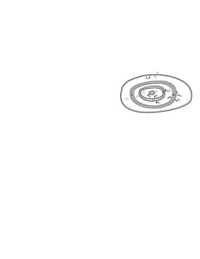
Figure 2: A chain of embedded conductors with $N=3$. The surfaces $S_{2}$,$S_{3}$, have an inner and an outer part.

Let us study a set of $N+1$ conductors which are successively embedded. We label them $k=1,\ldots,N+1$ from the inner to the outer. Observe that the surface $S_{k}$ for each conductor with $k=2,\ldots,N$ has an inner and an outer part, but for $S_{N+1}$ we only define an inner part and for $S_{1}$ we only define an outer part (see Fig. 2). In addition, we define $V_{k}$ with $k=1,\ldots,N\$as the volume formed by the points exterior to the conductor $k$ and interior to the cavity of the conductor $k+1$ that contains the conductor $k$. Let us examine the non-diagonal elements $C_{km}$ assuming from now on that $k<m$.

From Eq. (1) we see that if $m-k=1$ then $f_{m}\left(S_{k}\right)=0$ and $f_{m}\left(S_{k+1}\right)=1$ because $S_{k+1}=S_{m}$, the volume $V_{k}$ is precisely delimited by the outer part of the surface $S_{k}$ and the inner part of the surface $S_{k+1}$; thus $f_{m}$ has a non-trivial solution in $V_{k}$. Therefore, we have in general that $\nabla f_{m}\neq 0$ in $V_{k}$ and in the surfaces that delimite it. Thus the integral

$$C_{km}=-\varepsilon_{0}\oint\limits_{S_{k}}\nabla f_{m}\cdot\mathbf{n}_{k}~{}dS$$ (56)

has a contribution from the outer part of $S_{k}$. Now, if $V_{k-1}$ exists (i.e. if $k>1$), and taking into account that $f_{m}\left(S_{k-1}\right)=f_{m}\left(S_{k}\right)=0$, the uniqueness theorem says that the only solution in $V_{k-1}$ is $f_{m}=0$ and hence $\nabla f_{m}=0$ in this volume and in the surfaces that delimite such a volume. Thus the integral surface in (56) has no contributions from the inner part of $S_{k}$.

Now, if $m-k\geq 2$ we see that $f_{m}\left(S_{k}\right)=f_{m}\left(S_{k+1}\right)=0$, then the only solution in $V_{k}$ is $f_{m}=\nabla f_{m}=0$ in this volume and in the surfaces that delimite such a volume. Thus the integral surface in (56) has no contributions from the inner part of $S_{k}$. On the other hand, if $V_{k-1}$ exists ($k>1$), and since $f_{m}\left(S_{k-1}\right)=f_{m}\left(S_{k}\right)=0$ we see once again that $f_{m}=\nabla f_{m}=0$ in the volume $V_{k-1}$ and in the surfaces that delimite it; so the integral (56) has no contribution from the outer part of $S_{k}$ either.

From the previous discussion and appealing to the symmetry of the e-matrix, we conclude that $C_{km}=0$ for $\left|m-k\right|\geq 2$. In addition, when $\left|m-k\right|=1$, the surface integral (56) receives contribution only from the outer part of $S_{k}$. Notice that the previous behavior has to do with the fact that the total volume $V_{S_{T}\text{ }}$ consists of several disjoint (and so disconnected) regions and that $\left|k-m\right|\geq 2$ indicates that these labels are always associated with disjoint volumes. In the last discussion we have not included the possibility that the most interior conductor has a cavity. Since it would be an empty cavity, the surface and volume of this cavity do not contribute to the calculation of any coefficient of capacitance (see Ref. [27]).

From the results above, we see that for $N+1$ successively embedded conductors with $N\geq 2$, we have

$$C_{ii} = -\left(C_{i,i-1}+C_{i,i+1}\right)\ \ ;\ \ i=2,\ldots,N$$

$$C_{11} = -C_{12}\ \ ;\ \ C_{N+1,N+1}=-C_{N,N+1}$$

How many degrees of freedom do we have for the e-matrix?.

Appendix D Suggested Problems

For checking the comprehension of the present formulation and its advantages, we give some general suggestions for the reader.

1. Show all the properties stated here for the r-matrix and e-matrix with specific examples.

2. Look for differences and similarities between the matrix of capacitance in electrostatics and the inertia tensor in mechanics, from the physical and mathematical point of view.

3. From $\left(\mathbf{\phi,c\phi}\right)\equiv k$ we find $\left(\mathbf{u},\mathbf{cu}\right)=1$ with $\mathbf{u}\equiv\phi/\sqrt{k}$. This defines the equation of an ellipsoid, describe how to find the length of the axes of the ellipsoid in the $\Phi^{N}$ and $\Phi^{N+1}$ spaces for the r-matrix and the e-matrix respectively. Describe the principal axes in these “potential spaces”.

4. By setting $\partial u/\partial\varphi_{i}=0$, prove that in the absence of constraints, the only local minimum of the internal energy is given by sets of the type $\phi_{0}$.

5. Prove Eq. (41) for the minimal internal energy under the constraint of constant internal charge.

6. Let $\left\{a,b\right\}\$be two positive numbers. Consider the $4\times 4$ matrix given by

   $$\mathbf{C}_{4\times 4}=\left(\begin{array}[]{cc}a\mathbf{B}_{2\times 2}&\mathbf{0}_{2\times 2}\\ \mathbf{0}_{2\times 2}&b\mathbf{B}_{2\times 2}\end{array}\right)\ \ ;\ \mathbf{B}_{2\times 2}\equiv\left(\begin{array}[]{cc}1&-1\\ -1&1\end{array}\right)$$

   this is a sp-matrix in which the sum of elements in each row is zero. Further, $\lambda=0$ is a two-fold degenerate eigenvalue of $\mathbf{C}$. Can $\mathbf{C}$ be a matrix of capacitance associated with a given electrostatic set of conductors?.

7. Look up for more applications of singular positive and positive-definite matrices in different contexts of Physics.

References

- [1] V. A. Erma, Perturbation Approach to the Electrostatic Problem for Irregularly Shaped Conductors, J. Math. Phys. 4 (1963) 1517-1526.
- [2] W. R. Smythe, Charged Spheroid in Cylinder, J. Math. Phys. 4 (1963) 833-837 .
- [3] R. Cade, Approximate capacities of some toroidal condensers, J. Phys. A: Math. Gen. 13(1980) 333-346.
- [4] M. Uehara, Green’s functions and coefficients of capacitance, Am. J. Phys. 54 (1986) 184-185.
- [5] G. J. Sloggett, N. G. Barton and S. J. Spencer, Fringing fields in disc capacitors, J. Phys. A: Math. Gen. 19(1986) 2725-2736.
- [6] V. Lorenzo and B. Carrascal, Green’s functions and symmetry of the coefficients of a capacitance matrix, Am. J. Phys. 56 (1988) 565.
- [7] H. J. Wintle, A note on capacitors with wide electrode separation, J. Phys. A: Math. Gen. 25 (1992) L639-L642.
- [8] E. Bodegom and P. T. Leung, A surprising twist to a simple capacitor problem, Eur. J. Phys. 14 (1993) 57-58.
- [9] C. Donolato, Approximate evaluation of capacitances by means of Green’s reciprocal theorem, Am. J. Phys. 64 (1996) 1049-1054.
- [10] Y. Cui, A simple and convenient calculation of the capacitance for an isolated conductor plate, Eur. J. Phys. 17 (1996) 363-364.
- [11] G. P. Tong, Electrostatics of two conducting spheres intersecting at angles, Eur. J. Phys. 17 (1996) 244-249.
- [12] H. J. Wintle, The capacitance of the cube and square plate by random walk methods, Journal Electrostat. 62 (2004) 51-62.
- [13] D. Palaniappan, Classical image treatment of a geometry composed of a circular conductor partially merged in a dielectric cylinder and related problems in electrostatics, J. Phys. A: Math. Gen. 38 (2005) 6253-6270.
- [14] S. Ghosh and A. Chakrabarty, Estimation of capacitance of different conducting bodies by the method of rectangular subareas, J. Electrostat. 66 (2008) 142-146.
- [15] Y. Xiang, Further study on electrostatic capacitance of an inclined plate capacitor, Journal Electrostat. 66 (2008) 366-368.
- [16] F. Ninio, A simple proof of the Perron-Frobenius theorem for positive symmetric matrices, J. Phys. A: Math. Gen. 9 (1976) 1281-1282.
- [17] A. Ray, Sufficient conditions for weak minimum of a functional depending on n functions and their derivatives, J. Math. Phys. 24(1983) 1395-1398.
- [18] R. Simon , S. Chaturvedi and V. Srinivasan, Congruences and canonical forms for a positive matrix: Application to the Schweinler–Wigner extremum principle, J. Math. Phys. 40 (1999) 3632-3642.
- [19] M. J. W. Hall, Complete positivity for time-dependent qubit master equations, J. Phys. A: Math. Theor. 41 (2008) 205302.
- [20] J. Wilkieand Y. M. Wong, Sufficient conditions for positivity of non-Markovian master equations with Hermitian generators, J. Phys. A: Math. Theor. 42 (2009) 015006.
- [21] H. Goldstein, C. Poole, J. Safko, Classical Mechanics, 3rd ed. Addison-Wesley, San Francisco, 2002.
- [22] C. Cohen-Tannoudji, B. Diu, F. Lalöe, Quantum Mechanics, John Wiley & Sons 2005, Hermann, Paris,1977.
- [23] W. T. Scott, The Physics of Electricity and Magnetism, 2nd ed. John Wiley & Sons, N. Y. 1966.
- [24] A. N. Matveev, Electricity and Magnetism, Mir, Moscow, 1988.
- [25] J. D. Jackson, Classical Electrodynamics, 3rd ed. John Wiley & Sons, N. J. 1998.
- [26] D. J. Griffiths, Introduction to Electrodynamics, 3rd ed. Prentice Hall, N. J. 1999.
- [27] W. J. Herrera and R. A. Diaz, The geometrical nature and some properties of the capacitance coefficients based on Laplace’s equation, Am. J. Phys. 76 (2008) 55-59.