Ingredients of a Casimir Analog Computer

Abstract

We present the basic ingredients of a technique to compute quantum Casimir forces at micrometer scales using antenna measurements at tabletop (e.g. centimeter) scales, forming a type of analog computer for the Casimir force. This technique relies on a correspondence that we derive between the contour integration of the Casimir force in the complex frequency plane and the electromagnetic response of a physical dissipative medium in a finite real-frequency bandwidth.

Casimir forces arise due to quantum fluctuations of the electromagnetic field Casimir (1948) and can play a significant role in the physics of neutral, macroscopic bodies at micrometer separations, such as in new generations of microelectronic mechanical systems (MEMS) Serry et al. (1998); Chan et al. (2001). These forces have previously been studied both in delicate experiments at micron and sub-micron lengthscales Bordag et al. (2001) and also in theoretical calculations that are only recently becoming feasible for complex non-planar geometries Emig et al. (2006); Rodriguez et al. (2006). Here, we propose a third alternative by deriving an equivalence between quantum fluctuations and the classical electromagnetic response in bodies separated by a conducting fluid, as illustrated in Fig. 1. Using this equivalence, we propose the possibility of experimental $S$-matrix measurements for microwave antennas in centimeter-scale models that indirectly yield the Casimir force between micron-scale objects. Such a centimeter-scale model is not a Casimir “simulator,” in that one is not measuring forces, but rather a quantity that is mathematical related to the micron-scale Casimir force—in this sense, it is a kind of analog computer. We believe that this mathematical equivalence between disparate quantum and classical systems reveals new opportunities for the experimental and theoretical study of Casimir interactions.

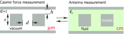
Figure 1: Schematic illustration of correspondence between observations of Casimir forces at $\mu$m lengthscales and antenna measurements of the electromagnetic response functions at tabletop lengthscales (e.g. cm).

In the following letter, we first review a well-known formulation of the Casimir force in terms of the classical Green’s function (GF) via the electromagnetic stress tensor (ST) and the fluctuation-dissipation theorem Lifshitz and Pitaevskii (1980). Although this formulation is normally expressed for either real or imaginary frequencies, we consider the general complex-frequency ($\omega$) plane. We then show that the mapping to complex frequency is equivalent to a real-frequency GF with a transformed electromagnetic medium $\varepsilon_{c}$. From this point of view, however, it turns out that only certain contours in the complex-frequency plane correspond to physically realizable $\varepsilon_{c}$, and in particular the real and imaginary frequency axes are unsuitable. Instead, we identify another contour and show its equivalence to a conventional conducting medium, demonstrate that the response of such a medium yields the correct Casimir force in nontrivial geometries, and consider the implications and possible materials for practical experiments. The key point is that, once the Casimir force is expressed in terms of the response of a realizable medium over a reasonably narrow bandwidth, the scale-invariance of Maxwell’s equations permits this response to be measured at any desired lengthscale, e.g. in a tabletop microwave experiment.

The Casimir force can be expressed as an integral of the mean electromagnetic ST over all frequencies Lifshitz and Pitaevskii (1980). The mean ST is determined simply from the classical GF (the fields in response to current sources at a fixed frequency), thanks to the fluctuation-dissipation theorem. It turns out, however, that this frequency integral is badly behaved from the perspective of numerical calculations (or experiments, below). Fortunately, because the integrand is analytic, one can deform the integration contour into the complex-frequency $\omega$ plane.

More generally, given an arbitrary contour $\omega(\xi)$ (for convenience below, we parameterize the contour by a real $\xi$), the force in the $i$-th coordinate direction is given by:

$$F_{i}=\operatorname{Im}\int_{0}^{\infty}d\xi\frac{d\omega}{d\xi}\oiint_{\mathrm{surface}}\sum_{j}\langle T_{ij}(\mathbf{r},\omega)\rangle\,dS_{j}\,.$$ (1)

The standard Wick rotation corresponds to the particular choice $\omega(\xi)=i\xi$ and yields a smooth and rapidly decaying integrand Rodriguez et al. (2006). The mean ST $\langle T_{ij}\rangle$ is related to the electric ($\mathbf{E}$) and magnetic ($\mathbf{H}$) field correlation functions by the standard equation (assuming non-magnetic materials, $\mu=1$, for simplicity):

$$\left\langle T_{ij}(\mathbf{r},\omega)\right\rangle=\left\langle H_{i}(\mathbf{r})\,H_{j}(\mathbf{r})\right\rangle-\frac{1}{2}\delta_{ij}\sum_{k}\left\langle H_{k}(\mathbf{r})\,H_{k}(\mathbf{r})\right\rangle\\ +\varepsilon(\mathbf{r},\omega)\Big{[}\left\langle E_{i}(\mathbf{r})\,E_{j}(\mathbf{r})\right\rangle-\frac{1}{2}\delta_{ij}\sum_{k}\left\langle E_{k}(\mathbf{r})\,E_{k}(\mathbf{r})\right\rangle\Big{]}\,.$$ (2)

The field correlation functions are, in turn, related to the frequency-domain classical photon GF, $G_{ij}(\omega;\mathbf{r},\mathbf{r}^{\prime})$, by the fluctuation-dissipation theorem:

$$\left\langle E_{i}(\mathbf{r})E_{j}(\mathbf{r}^{\prime})\right\rangle=\frac{\hbar}{\pi}\omega^{2}G_{ij}(\omega;\mathbf{r},\mathbf{r}^{\prime})$$ (3)

$$\left\langle H_{i}(\mathbf{r})H_{j}(\mathbf{r}^{\prime})\right\rangle=-\frac{\hbar}{\pi}(\nabla\times)_{i\ell}(\nabla^{\prime}\times)_{jm}G_{\ell m}(\omega;\mathbf{r},\mathbf{r}^{\prime})\,,$$ (4)

where $G_{ij}$ satisfies Maxwell’s equations:

$$\left[\nabla\times\nabla\times{}-\varepsilon(\mathbf{r},\omega)\omega^{2}\right]\mathbf{G}_{j}(\omega;\mathbf{r},\mathbf{r}^{\prime})=\delta(\mathbf{r}-\mathbf{r}^{\prime})\hat{\mathbf{e}}_{j}$$ (5)

Equation (5) can be solved in a number of ways, for example by a finite-difference discretization Rodriguez et al. (2006) or even analytically in one dimension Lifshitz and Pitaevskii (1980). Of course, the diagonal ($\mathbf{r}^{\prime}=\mathbf{r}$) part of the GF is formally infinite, but this singularity is not relevant because its surface integral is zero, and it is typically removed by some regularization (e.g. by the finite discretization or by a finite antenna size in the proposed experiments below). A crucial step, as mentioned above, is the passage to imaginary frequencies $\omega(\xi)=i\xi$. For real frequencies, the GF is oscillatory, leading to a highly oscillatory ST integrand that does not decay—even when a regularization (ultraviolet cutoff) is imposed, integrating a highly oscillatory function over a broad bandwidth is problematic. For imaginary frequencies, on the other hand, the GF is exponentially decaying, due to the operator in Eq. (5) becoming positive-definite ($\nabla\times\nabla\times{}+\varepsilon\xi^{2}$) Rodriguez et al. (2006), leading to a decaying non-oscillatory integrand.

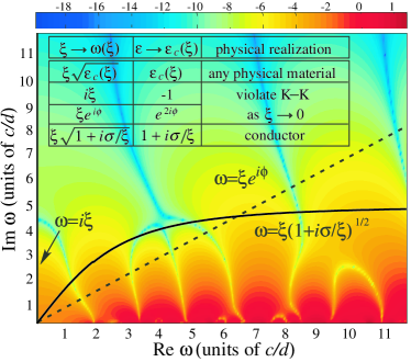
Figure 2: Complex-frequency $\omega$ plot of the Casimir force integrand ($\ln|\operatorname{Re}dF_{x}/d\omega|$), where $dF_{x}/d\omega$ is in units of $\hbar/d^{2}$, for the geometry of Fig. 1. As the real-$\omega$ axis is approached, the integrand becomes highly oscillatory, which is only partially revealed here due to the finite frequency resolution. Various integration contours of interest are labelled as black and dashed lines. (Inset:) Vacuum $\varepsilon=1$ contour deformations $\omega(\xi)$ and their corresponding (real-frequency) physical realizations $\varepsilon_{c}(\xi)$.

However, the Wick rotation is not the only contour in the complex plane that leads to a well-behaved decaying integrand. This is illustrated by Fig. 2, which shows the force integrand in the complex plane for the piston-like geometry of Fig. 1. In particular, we calculate the ($x$-direction) force integrand $dF_{x}/d\omega=\oiint_{\mathrm{surf}}\sum_{j}T_{xj}(\mathbf{r},\omega)dS_{j}$ on one square, for geometric parameters $h=0.5d$ and $s=d$, where $d$ is the separation between the blocks. Here, we plot $\ln|\operatorname{Re}dF_{x}/d\omega|$, which illustrates the basic features of the integrand $d\omega/d\xi\,dF_{x}/d\omega$ ($\operatorname{Im}dF_{x}/d\omega$ is also important, but is qualitatively similar). As described above, this integrand is oscillating along the $\operatorname{Re}\omega$ axis and decaying along the $\operatorname{Im}\omega$ axis, but it also decays along any contour where $\operatorname{Im}\omega$ is increasing (such as the three contours shown, to be considered in more detail below).

The fact that $\omega$ and $\varepsilon$ only appear together in Eq. (5), as $\varepsilon\omega^{2}$, immediately suggests that, instead of changing $\omega$ to a complex number, we can instead operate at real frequencies by transforming $\varepsilon$. In particular, a complex $\omega(\xi)$ is equivalent to a real frequency $\xi$ with a complex $\varepsilon$, where the imaginary part of $\varepsilon$ corresponds to dissipation loss. Thus, an intuitive explanation for why transforming to the complex-frequency plane was numerically useful above is simply that it corresponds to lossy materials that damp out the oscillations. Given a medium $\varepsilon$ at a complex frequency $\omega(\xi)$ where we wish to compute the ST for the Casimir force, we will transform to an equivalent problem at a real frequency $\xi$ and complex permittivity $\varepsilon_{\mathrm{c}}$. Namely, operating at a complex frequency $\omega(\xi)$ is clearly equivalent (for the photon GF) to operating at a real frequency $\xi$ and transforming a given material via $\varepsilon(\xi)\to\varepsilon(\omega)\omega^{2}/\xi^{2}=\varepsilon_{\mathrm{c}}$. Conversely, any frequency-dependent material $\varepsilon_{\mathrm{c}}(\xi)$ at a given point in space can be related to the GF for vacuum ($\varepsilon=1$) at that point by going from the real frequency $\xi$ to a complex frequency $\omega=\xi\sqrt{\varepsilon_{\mathrm{c}}(\xi)}$.

Because the ST is expressed in terms of the GF, and the GF at microwave lengthscales is merely a rescaling of the GF at micron lengthscales (if suitable materials can be found), one can conceivably measure the GF in an experiment via the $S$-matrix elements of antennas at centimeter scales, and so determine the Casimir force via integration of the ST. The passage to complex frequencies is essential here, as in numerics, because measuring the real-frequency GF will yield a highly oscillatory force integrand over an infinite bandwidth, imposing significant experimental challenges. Unfortunately, it is difficult to implement complex frequency deformations directly, because a complex frequency corresponds to fields and sources with exponential growth in time. An alternative, suggested by the correspondence above, is to measure the real-frequency GF of a physical medium with a complex permittivity $\varepsilon_{c}(\xi)=\varepsilon(\omega)\omega^{2}/\xi^{2}$. This $\varepsilon_{c}$ medium should satisfy two properties: it should correspond to an $\omega$ contour where the ST integrand is rapidly decaying, and it should be physically realizable. For simplicity, we begin by considering complex contours for the ST in vacuum ($\varepsilon=1$). The extension to arbitrary geometries/materials is straight-forward: an arbitrary inhomogeneous medium $\varepsilon(\mathbf{r},\xi)$ corresponds to $\varepsilon_{c}=\omega^{2}\varepsilon(\mathbf{r},\omega)/\xi^{2}$.

If $\varepsilon_{c}(\xi)$ is to correspond to a physical medium, it must satisfy the complex-conjugate property $\varepsilon_{c}(-\xi)=\varepsilon_{c}(\xi)^{*}$ as well as the Kramers–Kronig (K–K) relations Jackson (1998). It is most important to satisfy these conditions for small $\xi$, since the ST integrand is dominated by long-wavelength contributions. One should also prohibit gain media, which would lead to the exponentially growing fields we are trying to avoid by not using complex $\omega$. For example, Wick rotations correspond to $\varepsilon_{c}(\xi)=-1$, and this is only possible at $\xi=0$ in a gain medium, since in a dissipative medium, $\varepsilon_{c}$ is real and positive along the whole imaginary-$\xi$ axis (this is implied by K–K). The generalization to arbitrary rotations in the complex plane $\varepsilon=e^{2i\phi}$ is both a gain medium and violates $\varepsilon_{c}(-\xi)=\varepsilon_{c}(\xi)^{*}$ near $\xi=0$. Thus, no realizable material can emulate these contours even in a narrow bandwidth around $\xi=0$, as summarized on the table (inset) of Fig. 2.

Although traditional Wick rotations correspond to unphysical materials, there are obviously many physical lossy materials to choose from, each of which corresponds to a contour in the complex plane, and one merely needs to find such a “physical” contour on which the ST is rapidly decaying so that experiments can be performed over reasonable bandwidths. A simple and effective lossy material for this purpose is a conductor with conductivity $\sigma$. Because the integral will turn out to be dominated by the contributions near zero frequency, it is sufficient to consider $\sigma$ to be a constant (the DC conductivity), although of course the full experimental permittivity $\varepsilon_{c}(\xi)$ could also be used. Specifically, consider the general class of conductors defined by dispersion relations of the form $\varepsilon_{c}(\xi)=1+i\sigma/\xi$, corresponding to vacuum with a complex contour $\omega_{\sigma}=\xi\sqrt{1+i\sigma/\xi}$. As shown in Fig. 2, the integrand of this contour is in fact well behaved, rapidly decaying and exhibits few oscillations.

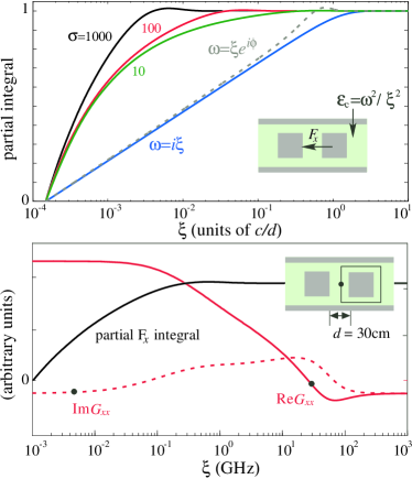
Figure 3: (Top:) Partial force integral $\int_{0}^{\xi}dF_{x}$, normalized by $F_{x}$, as a function of $\xi$, for the various $\omega(\xi)$-contours (equivalently, various $\varepsilon_{c}=\omega^{2}/\xi^{2}$) shown in Fig. 3. The solid green, red and black lines correspond to conductive media with $\sigma=10$, $10^{2}$ and $10^{3}$, respectively ($\sigma$ has units of $c/d$). The dashed grey and solid blue lines correspond to $\phi=\pi/4$ and $\phi=\pi/2$ (Wick) rotations. (Bottom:) Illustration of the required frequency bandwitdth for a possible realizations using saline solution at separation $d=30$cm. The red lines plot the $xx$-component of the photon GF $G_{xx}$ at a single location on the surface contour (see inset) as a function of $\xi$ (GHz). The black line is the corresponding partial force integrand.

We now consider the Casimir force for the same structure as in Fig. 1, still calculated by the same finite-difference method as in Fig. 3, but we now focus on the properties along different contour choices for both physical and unphysical media. In particular, Fig. 2(top) plots the partial integral $\int_{0}^{\xi}(d\omega/d\xi)(dF_{x}/d\omega)d\xi$, normalized by the total force $\int_{0}^{\infty}dF_{x}$, as a function of $\xi$. [As it must, the total integral over $\xi$, the force $F_{x}$, is invariant regardless of the contour $\omega(\xi)$ and agrees with previous results Rodriguez et al. (2006); Specifically, $F_{x}=0.0335$ $(\hbar c/d^{3})$.] We now comment on two important features of the $\omega_{\sigma}$ contour that are relevant to experiments.

First, the Jacobian factor for $\omega_{\sigma}$ is given by $d\omega_{\sigma}/d\xi=0.5(2+i\sigma/\xi)/\sqrt{1+i\sigma/\xi}$ and turns out to be very important at low $\xi$. The ST integrand itself goes to a constant as $\xi\to 0$ (due to the constant contribution of zero-frequency modes), but the Jacobian factor diverges in an integrable square-root singularity $\sim\sqrt{\sigma/\xi}$. Since this singularity is known analytically, however, separate from the measured or calculated GF, integrating it accurately poses no challenge. Second, the larger the value of $\sigma$, the more rapidly the ST integrand decays with $\xi$, and as a consequence the force integral for larger $\sigma$ is dominated by smaller $\xi$ contributions. In comparison, previous calculations of Casimir forces along the imaginary-frequency axis revealed that the relevant $\xi$ bandwidth was determined by some characteristic lengthscale of the geometry such as body separations Rodriguez et al. (2006). Here, we have introduced a new parameter $\sigma$ that can squeeze the relevant $\xi$ bandwidth into a narrower region. This “spectral squeezing” effect is potentially useful for experiments, as it partially decouples the experimental lengthscale of the geometry from the required frequency bandwidth.

As a consequence of the above results, we can now outline a possible experiment at centimeter lengthscales that determines the Casimir force at micron lengthscales, a Casimir analog computer (CAC). Suppose that one wishes to compute the Casimir force between perfect-metal objects separated by vacuum, such as the geometry in Fig. 1. One would then construct a scale model of this geometry at a tabletop scale (e.g., centimeters) out of metallic objects (which can be treated as perfect metals at microwave and longer wavelengths). To determine the ST integrand along a complex-$\omega_{\sigma}$ contour, one would measure the GF at real frequencies $\xi$ for the model immersed in a conducting fluid. The GF is related to the $S$-matrix of pairs of antennas, and the diagonal of the GF to the $S$-matrix diagonal of a single antenna [noting that the finite size of the antenna automatically regularizes the integrand, as noted after Eq. (5)]. It is important for the model structure to be large enough that the introduction of a small dipole-like antenna does not significantly alter the electromagnetic response. In general, the ST must be integrated in space over a closed surface around the object, and correspondingly the antenna’s $S$-matrix spectrum must be measured at a number of antenna positions (2d quadrature points) around this surface. (Unless one is interested in computing the force on a single atom, which requires a single antenna measurement.) The different components of the GF tensor correspond to different antenna orientations. The magnetic GF can be determined from the photon GF by Eq. (3), or possibly by employing“magnetic dipole” antennas formed by small current loops.

We now consider a particular CAC (at the cm scale) that employs realistic geometric and material parameters. Many available fluids exhibit almost exactly the desired material properties from above. One such example is saline water, which has $\varepsilon(\xi)=\varepsilon_{s}+i\sigma/\xi$, where $\varepsilon_{s}\approx 80$ and $\sigma\approx 5$ S/m for relatively small values of salt concentration Klein and Swift (1977). A calculation using these parameters, based on the geometry of Fig. 1, assuming object sizes and separations at the centimeter to meter scale (we choose $d=0.3$ m for the structure in Fig. 1, corresponding to a frequency of 1 GHz), reveals that it is only required to integrate the stress tensor up to small GHz frequencies $\xi$, which is well within the reach of conventional antennas and electronics. This is illustrated in Fig. 3(bottom), which plots the $G_{xx}$ component of the GF (red lines) as well as the partial force integrand (black line), showing the high $\xi<1$ GHz cancellations that occur once the ST is integrated along a surface (inset). We note that most salts exhibit additional dispersion for $\xi>10$ GHz Klein and Swift (1977), but we do not need to reach those frequency scales. (Nevertheless, should there be substantial dispersion in the conducting fluid, one could easily take it into account as a different complex-$\omega$ contour.)

Some attention to detail is required in applying this correspondence correctly. For instance, using network analyzers, what is measured in such an experiment is not the photon GF $\mathbf{G}$, but rather the electric $S$-matrix $\mathbf{S}^{E}$ (the currents in a set of receiver antennas due to currents in the source antennas) , related to the electric GF (the $\mathbf{E}$-field response to an electric current $\mathbf{J}$) by a factor depending on the antenna geometry alone (relating $\mathbf{J}$ to $\mathbf{E}$). The electric GF will differ from the photon GF by a factor of the real frequency $i\xi$. To summarize, the photon GF will be given in terms of the measured $\mathbf{S}^{E}$ by $G_{ij}(\omega)=(\alpha/i\xi)S^{E}_{ij}(\xi)$, where $\alpha$ is the antenna-dependent geometric factor. To obtain the ST from $G_{ij}$, one multiplies by factors of $\omega(\xi)^{2}$ as in Eq. (3). Figure 3(bottom) illustrates the expected behavior of $S_{xx}\sim G_{xx}/\xi$ in a realistic system employing a sline solution with $d=30$cm.

The use of tabletop models and analog computers in physics, though rarely explored in the context of vacuum fluctuations, continues to play an important role in contemporary research fields, such as quantum information Lloyd (2008). Especially for three-dimensional geometries, tabletop experiments offer a route to rapidly exploring many different geometric configurations that remain extremely challenging for conventional numerical calculation. Although many details of such an experiment remain to be developed, we believe that the basic ingredients are both clear and feasible, at least when restricted to perfect-metal bodies. The most difficult case to realize seems to be the force between imperfect-metal or dielectric bodies with a permittivity $\varepsilon(\omega)$, as the corresponding tabletop system requires materials with a specified dispersion relation $\varepsilon_{c}^{\mathrm{body}}(\xi)/\varepsilon_{c}^{\mathrm{fluid}}(\xi)=\varepsilon(\omega(\xi))$ relative to the conducting fluid. This may be an opportunity for specially designed meta-materials with the desired frequency response.

We are grateful to Zheng Wang and Peter Shor at MIT, and to Jeremy Munday at Caltech for useful discussions. This work was supported by the Army Research Office through the ISN under Contract No. W911NF-07-D-0004, the MIT Ferry Fund, and by US DOE Grant No. DE-FG02-97ER25308 (ARW).

References

- Casimir (1948) H. B. G. Casimir, Proc. K. Ned. Akad. Wet. 51, 793 (1948).
- Serry et al. (1998) F. M. Serry, D. Walliser, and M. G. Jordan, J. Appl. Phys. 84, 2501 (1998).
- Chan et al. (2001) H. B. Chan, V. A. Aksyuk, R. N. Kleinman, D. J. Bishop, and F. Capasso, Science 291, 1941 (2001).
- Bordag et al. (2001) M. Bordag, U. Mohideen, and V. M. Mostepanenko, Phys. Rep. 353, 1 (2001). R. Onofrio, New J. Phys. 8, 237 (2006).
- Rodriguez et al. (2006) A. Rodriguez, M. Ibanescu, D. Iannuzzi, J. D. Joannopoulos, and S. G. Johnson, Phys. Rev. A 76, 032106 (2007).
- Emig et al. (2006) T. Emig, R. L. Jaffe, M. Kardar, and A. Scardicchio, Phys. Rev. Lett. 96, 080403 (2006). A. Lambrecht, N. Maia, A. Paulo, and S. Reynaud, New J. Physics 8, 243 (2006). H. Gies and K. Klingmuller, Phys. Rev. D 74, 045002 (2006). T. Emig, N. Graham, R. L. Jaffe, and M. Kardar, Phys. Rev. Lett. 99, 170403 (2007).
- Lifshitz and Pitaevskii (1980) E. M. Lifshitz and L. P. Pitaevskii, Statistical Physics: Part 2 (Pergamon, Oxford, 1980).
- Jackson (1998) J. D. Jackson, Classical Electrodynamics (Wiley, New York, 1998), 3rd ed.
- Klein and Swift (1977) L. A. Klein and C. T. Swift, IEEE Trans. Ant. and Prop. 25, 104 (1977).
- Lloyd (2008) S. Lloyd, Science 319, 1209 (2008).