Analysis of a threshold model of social contagion on degree-correlated networks.

Abstract

We analytically determine when a range of abstract social contagion models permit global spreading from a single seed on degree-correlated, undirected random networks. We deduce the expected size of the largest vulnerable component, a network’s tinderbox-like critical mass, as well as the probability that infecting a randomly chosen individual seed will trigger global spreading. In the appropriate limits, our results naturally reduce to standard ones for models of disease spreading and to the condition for the existence of a giant component. Recent advances in the distributed, infinite seed case allow us to further determine the final size of global spreading events, when they occur. To provide support for our results, we derive exact expressions for key spreading quantities for a simple yet rich family of random networks with bimodal degree distributions.

Over the last decade, the study of real-world, complex networks has grown enormously, fueled in no small part by the advent of readily available, large-scale data sets for real systems (Newman, 2003a; Boccaletti et al., 2006). Understanding the coupled dynamics of both the structural evolution of, and processes on, complex networks remains a fertile area of investigation. Of particular importance is the study of contagion, how entities spread through networked systems, as exemplified by the diffusion of practices, beliefs, ideas, and emotions in social networks (Coleman et al., 1966; Hatfield et al., 1993; Fowler and Christakis, 2008), disease contagion in human and animal populations (Murray, 2002; Anderson and May, 1991), cascading failures in electrical systems (Sachtjen et al., 2000; Kinney et al., 2005), the global spread of computer viruses on the Web (Newman et al., 2002; Balthrop et al., 2004), and the collapse of financial systems (Sornette, 2003).

Our present interest lies in contagion processes where individuals adopt alternate behaviors through imitation of peers. We specifically investigate a threshold model of social contagion on random networks—first proposed and studied by Watts (Watts, 2002)—with the added complication of arbitrary degree-degree correlations. The model’s origins lie in the seminal work of Schelling, who employed a threshold model for a population on a checkerboard to gain insight into residential segregation (Schelling, 1971, 1978). Granovetter (Granovetter, 1978) subsequently studied a mean-field, random mixing threshold model which can be seen as a natural limiting case of the model we consider here. Both Schelling and Granovetter’s work clearly showed that global uniformity should not be taken to mean that individuals have strong or similar preferences, and that small changes in the distributions of individual preferences could lead to sharp transitions in the system’s macroscopic state.

Placing the threshold model on standard random networks with arbitrary degree distributions gives rise to a number of novel behaviors not seen in the Granovetter model. For example, individuals are now distinguishable, and a single node changing its state can lead to a complete transition in the entire system’s state Watts (2002). Moreover, by greatly limiting nodes’ knowledge of the complete network, behaviors that would immediately die out when nodes are aware of all other nodes’ states may now spread globally. Balkanization enhances innovation.

We consider binary systems with nodes being in one of two states, $\sigma_{0}$ and $\sigma_{1}$. Initially, all nodes are in state $\sigma_{0}$. Our immediate interest is in determining whether or not global spreading is possible when a single node is switched to state $\sigma_{1}$, and how this condition is affected by altering the level of degree-degree correlations. We then further wish to know two key quantities: (1) the probability global spreading occurs ($P_{\rm trig}$), and (2) when it does, to what fraction of the entire network ($S$).

In finding the probability that global spreading takes off after switching a single node to state $\sigma_{1}$, it is enough for us to view the problem as one of standard percolation (Stauffer and Aharony, 1992; Newman et al., 2001). (Determining the final extent of spreading requires a distinct approach but nevertheless still capitalizes on the locally branching nature of random networks (Gleeson and Cahalane, 2007; Gleeson, 2008).) This observation follows from several well known aspects of random networks.

First, infinite, sparse random networks are locally perfectly branching networks, possessing only very long cycles when sufficiently connected. Thus, a node can switch to state $\sigma_{1}$ in the initial stages of a spreading process (started by a single seed) only if a single neighbor switches to $\sigma_{1}$ earlier on. For global spreading to occur, a network must have a percolating component of these easily switched ‘vulnerable’ nodes (Watts, 2002). (By percolating component, we mean a connected sub-network containing a non-zero fraction of all nodes.) As the adoption of state $\sigma_{1}$ spreads through this percolating component of vulnerable nodes, non-vulnerable nodes requiring two or more neighbors in state $\sigma_{1}$ may also begin to switch. However, we need focus only on vulnerable nodes to determine whether global spreading is possible or not. When a percolating vulnerable component exists, it may be viewed as a network’s critical mass, and one that is highly susceptible since it possesses its own critical mass—exactly any one of its own members.

Second, our analytic treatment via generating functions is limited to the description of finite network components, which indirectly allows us to describe some aspects of infinite components. Since finite components are pure branching structures (i.e., they contain no cycles of any length), all nodes can only switch to $\sigma_{1}$ due to the conversion of a single neighbor, even in the long run.

We structure the paper as follows. After defining the model fully in Section I, we detail a series of analytic results in Section II, concerning the probability and size of macroscopic spreading events. We confirm, via further analysis and simulations, a number of our calculations for a simple network containing two kinds of nodes in Section III. We offer some concluding remarks in Section IV.

I Model definition

Each node is initially assigned a ‘response function’ which we take here to be a step function. In effect, each node is given a fixed threshold $\tau$ sampled from a distribution $P_{\rm threshold}(\tau)$. Node states update in synchrony at times $t=0$, 1, 2, …Each node observes the fraction of its neighbors in state $\sigma_{1}$, and switches to $\sigma_{1}$ if this fraction meets or exceeds its threshold, $\tau$. Once a node switches to state $\sigma_{1}$, it remains in state $\sigma_{1}$ permanently (akin to the SI model for disease spreading (Murray, 2002)). Asynchronous updating gives the same results for monotonically increasing response functions.

We define the structure of our networks through edge probabilities, following Newman (Newman, 2002, 2003b). In studying a range of structural aspects of degree-correlated networks as well as dynamic phenomena on them (especially contagion processes), it is mathematically convenient to use $e_{jk}$, the probability that a randomly chosen edge connects a node with degree $j+1$ to one with degree $k+1$, rather than $j$ and $k$. The quantity $e_{jk}$ then refers directly to the number of other edges emanating from the nodes an edge connects. Normalization is uncomplicated, requiring that $\sum_{j=0}^{\infty}\sum_{k=0}^{\infty}e_{jk}=1$.

While this definition of $e_{jk}$ is clear for directed networks, we encounter some subtleties in attempting to accommodate both undirected and directed networks with a single notation (even though many expressions will turn out to be the same). For undirected networks, which are our primary focus here, we evenly divide the probability that a randomly selected edge (now directionless) connects nodes with degree $j+1$ and $k+1$ between the quantities $e_{jk}$ and $e_{kj}$. The chance of a randomly selected edge connecting degree $j+1$ and $k+1$ nodes is then $e_{jk}+e_{kj}=2e_{jk}$, and the matrix formed by the $e_{jk}$ is symmetric. We are thus effectively retaining a ghost of a directed network, as each link must have a designated first and second node. (For directed networks, $e_{jk}$ need of course not be symmetric, and other complications are possible concerning the correlations between an individual node’s in-degree and out-degree.)

We also have the important quantity $q_{k}$ which is the probability that in randomly choosing an edge, and then randomly choosing one end of that edge, we arrive at a node of degree $k+1$ (equivalently, the node has $k$ emanating edges). For undirected networks, we have the derivation $q_{k}=\frac{1}{2}\sum_{j=0}^{\infty}e_{jk}+\frac{1}{2}\sum_{j=0}^{\infty}e_{kj}=\sum_{j=0}^{\infty}e_{jk}.$ (The same end expression holds for directed networks, where we must follow the edge’s direction.)

The Pearson correlation coefficient $r$ for degree pairs gives us a measure of assortativity, and is given by

$$r=\frac{1}{\sigma_{q}^{2}}\sum_{j=0}^{\infty}\sum_{k=0}^{\infty}{jk(e_{jk}-q_{j}q_{k})}$$ (1)

where $\sigma_{q}^{2}=\sum_{k}{k^{2}q_{k}}-[\sum_{k}{kq_{k}}]^{2}$ is the variance in the number of emanating edges from a node arrived at by a random edge. Note that the choice of $e_{jk}$ almost prescribes the form of the resulting network’s degree distribution, $p_{k}$. The one piece of information missing is the abundance of nodes with no connections, $p_{0}$, which we must define independently. A link between the $e_{jk}$ and $p_{k}$ for undirected networks follows from the observation that $q_{k}$ is readily determined from the degree distribution: a randomly chosen edge leads to a degree $k+1$ node with probability $q_{k}=(k+1)p_{k+1}/k_{\rm avg}$ where $k_{\rm avg}=\sum_{k=0}^{\infty}kp_{k}$ is the average degree. We therefore have the connection $q_{k}=\sum_{j=0}^{\infty}e_{jk}=(k+1)p_{k+1}/k_{\rm avg}.$ Now, in isolating the $p_{k}$, we do not need to know $k_{\rm avg}$. It is enough to know $p_{k}\propto q_{k}/(k+1)$ for $k>0$, since we can find the normalization constant (which is in fact $k_{\rm avg}$) by requiring $\sum_{k=1}^{\infty}p_{k}=1-p_{0}$.

Finding the probability of triggering a global spreading event reduces to standard percolation once we find the probability that an individual node is vulnerable. We allow this probability to be a function of node degree $k$, using the notation $b_{k1}$ (more generally, we write the probability that a node of degree $k$ switches to state $\sigma_{1}$ given $l$ contacts in state $\sigma_{1}$ as $b_{kl}$). We first determine whether nodes are vulnerable or not, removing them from the network in the latter case. Finally, if global spreading occurs on the resulting reduced network, global spreading must occur on the original network.

II Analytic results

Building on the work of Newman (Newman, 2002), we find closed form expressions for several probability generating functions related to component sizes. The key probability we need to characterize is $f_{n,j}$, which is the probability that an edge emanating from a degree $j+1$ node leads to a finite vulnerable subcomponent of size $n=0,1,2,\ldots$. Writing the marginal generating function for $f_{n,j}$ as $F_{j}(x;\vec{b}_{1})=\sum_{n=0}^{\infty}f_{n,j}x^{n}$, we have the following recursive relationship:

$$F_{j}(x;\vec{b}_{1}) =x^{0}\sum_{k=0}^{\infty}\frac{e_{jk}}{q_{j}}(1-b_{k+1,1})$$

$$+x\sum_{k=0}^{\infty}\frac{e_{jk}}{q_{j}}b_{k+1,1}\left[F_{k}(x;\vec{b}_{1})\right]^{k},$$ (2)

where $j=0,1,2,\ldots$. In both terms, we have the quantity $e_{jk}/q_{j}$ which represents the normalized probability that an edge from a degree node $j+1$ leads to a degree $k+1$ node. For undirected networks, we obtain this probability as $(e_{jk}+e_{kj})/(\sum_{k=0}^{\infty}e_{jk}+e_{kj})=2e_{jk}/2q_{j}=e_{jk}/q_{j}.$ The first term in Eq. (II) records the probability that an edge from a degree $j+1$ node leads immediately to a non-vulnerable node, and hence a vulnerable subcomponent of size $0$.

The second term involves a composition of generating functions. The generating function $F_{k}$ is the argument of

$$\sum_{k=0}^{\infty}\frac{e_{jk}}{q_{j}}b_{k+1,1}x^{k},$$ (3)

which is itself the generating function for the probability that an edge from a degree $j+1$ node leads to a vulnerable node with $k$ emanating edges foo . Finally, the $x$ leading the second term in Eq. (II) accounts for the $k+1$ degree node itself.

Our task is now to find critical points indicating the onset of a giant component as we vary network structure by altering the $e_{jk}$ and $b_{k1}$. We compute the average size of a finite vulnerable component found by following an edge from a degree $j+1$ node, given by $F_{j}^{\prime}(1;\vec{b}_{1})$. Differentiating Eq. (II), setting $x=1$, and substituting $q_{j}=\sum_{k=0}^{\infty}e_{jk}$, we have

$$q_{j}F_{j}^{\prime}(1;\vec{b}_{1})=\sum_{k=0}^{\infty}e_{jk}b_{k+1,1}+\sum_{k=0}^{\infty}ke_{jk}b_{k+1,1}F_{k}^{\prime}(1;\vec{b}_{1}).$$ (4)

(We have used the fact that $F_{k}(1;\vec{b}_{1})=1$ for networks without a giant component, and all components contribute to the generating function of $f_{n,k}$.) Rearranging Eq. (4), we have a linear system

$$\sum_{k=0}^{\infty}\left(\delta_{jk}q_{k}-kb_{k+1,1}e_{jk}\right)F_{k}^{\prime}(1;\vec{b}_{1})=\sum_{k=0}^{\infty}e_{jk}b_{k+1,1}$$ (5)

which we write as

$$\mathbf{A}_{\mathbf{E},\vec{b}_{1}}\vec{F}^{\prime}(1;\vec{b}_{1})=\mathbf{E}\vec{b}_{1}$$ (6)

where

$$\left[\mathbf{A}_{\mathbf{E},\vec{b}_{1}}\right]_{j+1,k+1} =\delta_{jk}q_{k}-kb_{k+1,1}e_{jk},$$ (7)

$$\left[\vec{F}^{\prime}(1;\vec{b}_{1})\right]_{k+1} =F_{k}^{\prime}(1;\vec{b}_{1}),$$ (8)

$$\left[\mathbf{E}\right]_{j+1,k+1} =e_{jk},$$ (9)

$$\mbox{and}\ \left[\vec{b}_{1}\right]_{k+1} =b_{k+1,1}$$ (10)

for $j$, $k$ = 0, 1, 2, 3, …. A solution exists when $\mathbf{A}_{\mathbf{E},\vec{b}_{1}}$ is invertible, i.e., its determinant is non-zero. We then have

$$\vec{F}^{\prime}(1;\vec{b}_{1})=\mathbf{A}_{\mathbf{E},\vec{b}_{1}}^{-1}\,\mathbf{E}\vec{b}_{1}.$$ (11)

Our condition for the onset of global spreading is therefore

$$\left|\mathbf{A}_{\mathbf{E},\vec{b}_{1}}\right|=0.$$ (12)

with $\mathbf{A}_{\mathbf{E},\vec{b}_{1}}$ defined in Eq. (7). We note that for networks where one or more degrees are not present (which we will encounter in our later specific examples), we omit the rows and columns of the above matrices corresponding to those degrees. For simplicity, we present our general results for networks assuming all degrees are represented, observing that adjustments to specific sets of degrees are straightforward.

For uncorrelated networks, upon substituting $e_{jk}=q_{j}q_{k}$, the above collapses to the known condition

$$\sum_{k=0}^{\infty}b_{k1}(k-1)\frac{kp_{k}}{k_{\rm avg}}=1,$$ (13)

as expected (Watts, 2002). Moreover, $F_{k}^{\prime}(1;\vec{b}_{1})$ is seen to be independent of $k$, since the first node of an edge is now unrelated to the other node and hence also the subcomponent it leads to. We provide details for these calculations in the Appendix.

Returning to the general case of degree-correlated networks, we see that when $b_{k1}=b$, a constant for all $k$, we have a disease-like contagion process. Furthermore, when $b=1$, all nodes are vulnerable, and we have found the condition for a giant component, equivalent to that obtained by Newman (Newman, 2002). (Note that when $b_{k1}=b$, we have $\mathbf{E}\vec{b}_{1}=b\vec{q}$ since $[\mathbf{E}\vec{b}_{1}]_{j+1}=\sum_{k=0}^{\infty}e_{jk}b_{k+1,1}=b\sum_{k=0}^{\infty}e_{jk}=bq_{j+1}$.)

We next consider two probability distributions pertaining to component size: (1) $g_{n}$, the probability that a randomly chosen node belongs to a vulnerable component of size $n$, and (2) $h_{n}$, the probability that a randomly chosen node belongs or is adjacent to a vulnerable component of size $n$. Knowing $g_{n}$ helps us find the size of the largest vulnerable component, whose presence or absence dictates whether or not global cascades are possible for infinite random networks. The second probability $h_{n}$ will aid us in determining the probability of triggering a global cascade. The triggering node, which is exogenously switched to state $\sigma_{1}$ may be either vulnerable and part of the largest vulnerable component, or non-vulnerable and connected to one or more nodes in the largest vulnerable component. For the standard giant component case where $b_{k1}=1$, we have $g_{n}=h_{n}$; otherwise, these distributions are likely distinct.

As for the $f_{k,n}$, we find closed form expressions for the generating functions associated with $g_{n}$ and $h_{n}$. The generating function for $g_{n}$ satisfies the following relationship:

$$G(x;\vec{b}_{1})= \,x^{0}\sum_{k=0}^{\infty}p_{k}(1-b_{k1})+x^{1}p_{0}b_{01}$$

$$+x\sum_{k=1}^{\infty}p_{k}b_{k1}\left[F_{k-1}(x;\vec{b}_{1})\right]^{k}.$$ (14)

The $x^{0}$ term carries the probability that a randomly selected node will not be in state $\sigma_{1}$; the second term accounts for the randomly chosen node being vulnerable but having degree 0; and the third term again uses the composition rule for sums of random variables of random sizes foo . The generating function $\sum_{k=1}^{\infty}p_{k}b_{k1}x^{k}$ corresponds to the probability distribution for a randomly chosen node to have degree $k$ and be vulnerable. Note that the argument $F_{k-1}$ appears in the last term rather than $F_{k}$ because $F_{k-1}$ by definition corresponded to a degree $k$ node.

The generating function for the triggering distribution satisfies a simplified version of Eq. (II):

$$H(x;\vec{b}_{1})=x^{1}p_{0}+x\sum_{k=1}^{\infty}p_{k}\left[F_{k-1}(x;\vec{b}_{1})\right]^{k}.$$ (15)

For the triggering distribution, the first node is now always switched to state $\sigma_{1}$, regardless of whether it is itself vulnerable or not. The $x^{1}$ term accounts for this initial node having degree 0 and hence being unable to trigger any other node. If the initial node has at least one neighbor, then spreading may occur and we can make use of the basic degree generating function $\sum_{k=1}^{\infty}p_{k}x^{k}$ combined with the generating function $F_{k-1}(x;\vec{b}_{1})$ for finite vulnerable subcomponent size. As per our previous examples, the preceding factor $x$ in the second term accounts for the initial node. In effect, $b_{k1}=1$ for the triggering node as it is always forced to be switched to state $\sigma_{1}$, and indeed setting $b_{k1}=1$ in Eq. (II) directly yields Eq. (15).

Now, the fraction of nodes in the largest vulnerable component is given by $S_{\rm vuln}=1-G(1;\vec{b}_{1})$, since $G(1;\vec{b}_{1})$ can be seen as the probability that a random node is part of a finite vulnerable component (including one of size 0). Setting $x=1$ in Eq. (II), we have

$$S_{\rm vuln}= 1-G(1;\vec{b}_{1})$$

$$= \sum_{k=0}^{\infty}p_{k}b_{k1}-p_{0}b_{01}-\sum_{k=1}^{\infty}p_{k}b_{k1}\left[F_{k-1}(1;\vec{b}_{1})\right]^{k}.$$ (16)

In the same fashion as for $S_{\rm vuln}$, the probability of triggering a cascade can be determined using $H(x;\vec{b}_{1})$:

$$S_{\rm trig}= 1-H(1;\vec{b}_{1})$$

$$= 1-\sum_{k=0}^{\infty}p_{k}\left[F_{k-1}(1;\vec{b}_{1})\right]^{k}.$$ (17)

The size of the triggering component can also be obtained by first making the observation that an initially switched node of degree $k$ triggers a cascade with probability

$$S_{\rm trig}^{(k)}=1-\left[F_{k-1}(1;\vec{b}_{1})\right]^{k}.$$ (18)

This is the probability that at least one edge from a degree $k$ node leads to a giant component of vulnerable nodes. We then have $S_{\rm trig}=\sum_{k=0}^{\infty}p_{k}S_{\rm trig}^{(k)},$ which is in agreement with Eq. (II).

Both $S_{\rm vuln}$ and $S_{\rm trig}$ depend on $F_{k}(1;\vec{b}_{1})$, for which we obtain a potentially infinite set of closed-form, coupled, nonlinear recursive expressions from Eq. (II):

$$F_{j}(1;\vec{b}_{1})=\sum_{k=0}^{\infty}\frac{e_{jk}}{q_{j}}(1-b_{k+1,1})+\sum_{k=0}^{\infty}\frac{e_{jk}}{q_{j}}b_{k+1,1}\left[F_{k}(1;\vec{b}_{1}\,)\right]^{k}$$ (19)

where we have substituted $q_{j}=\sum_{k=0}^{\infty}e_{jk}$. Solving Eq. (19) will almost always involve numerical techniques (though in Section III, we examine a case that has analytic solutions). The uncorrelated, pure random network version for the giant component ($b_{k1}=1$) may serve as some inspiration. There, we have no dependence on the degree of the initial node and the problem reduces to solving $F(1,\vec{1})=\sum_{k=0}^{\infty}q_{k}[F(1,\vec{1})]^{k}$. Both $F(1,\vec{1})=0$ and $F(1,\vec{1})=1$ are solutions and any initial estimate in between leads to, upon iteration, an intermediate solution, if one exists. Similarly, iteration of Eq. (19) should generally reach the appropriate fixed point solution.

We can also and more easily determine the average size of all vulnerable components (applicable when no giant vulnerable component is present since we again use $F_{k}(1;\vec{b}_{1})=1$):

$$G^{\prime}(1,\vec{b}_{1})=\vec{p}^{\rm T}\vec{b}_{1}+k_{\rm avg}(\mathbf{E}\,\vec{b}_{1})^{\rm T}\mathbf{A}_{\mathbf{E},\vec{b}_{1}}^{-1}\,(\mathbf{E}\,\vec{b}_{1}),$$ (20)

where $[\vec{p}]_{k}=p_{k}$. If we allow spreading to start from any node by forcing the first node to be in state $\sigma_{1}$, then the average size is instead given by

$$H^{\prime}(1,\vec{b}_{1})=1+k_{\rm avg}(\mathbf{E}\,\vec{1})^{\rm T}\mathbf{A}_{\mathbf{E},\vec{b}_{1}}^{-1}\,(\mathbf{E}\,\vec{b}_{1}).$$ (21)

We complete our analysis with a description of the expected final size of a global spreading event, when it occurs. We use the results of recent work by Gleeson and Calahane (Gleeson and Cahalane, 2007), and subsequently Gleeson (Gleeson, 2008), who have explicated an elegant, general solution to the distributed, infinite seed case for a variety of spreading models on a wide range of random networks.

Their key observation is that a node $i$ (degree $k_{i}$) switching to state $\sigma_{1}$ at time step $n$ can only be due to previous switching in nodes within $n$ steps of $i$ (including, trivially, $i$ itself). Furthermore, this neighborhood of $i$ must be a pure branching network, i.e., a tree rooted at $i$. At time step $n=1$, only $i$’s immediate neighbors influence $i$, and these are in state $\sigma_{1}$ with probability $\phi_{0}$. We write the probability that one of $i$’s edges connects to a node in state $\sigma_{1}$ at time step $n+1$ as $\theta_{k_{i},n}$. At time step $n=2$, the effect of next neighbors is felt, and $i$’s degree $k$ neighbors are now in state $\sigma_{1}$ with probability $\theta_{k,1}$ which in turn depends generally on $\theta_{k^{\prime},0}=\phi_{0}$, $k^{\prime}\geq 1$. Allowing $n$ to increase, we are lead to a recursive expression for the $\theta_{k,n}$ as follows. The expected size of a global spreading event given a fraction $\phi_{0}$ of nodes active at time $t=0$ is $\phi_{\infty}$, which is obtained in the $n\rightarrow\infty$ limit of the following equations (Gleeson, 2008):

$$\phi_{n+1}=\phi_{0}+(1-\phi_{0})\sum_{k=0}^{\infty}p_{k}\sum_{i=0}^{k}\binom{k}{i}\theta_{k,n}^{\,i}(1-\theta_{k,n})^{k-i}b_{ki}$$ (22)

where

$$\theta_{j,n+1}=\phi_{0}+(1-\phi_{0})\times$$

$$\sum_{k=1}^{\infty}\frac{e_{j-1,k-1}}{q_{j-1}}\sum_{i=0}^{k-1}\binom{k-1}{i}\theta_{k,n}^{\,i}(1-\theta_{k,n})^{k-1-i}b_{ki}$$

and, again, $\theta_{k,0}=\phi_{0}$ and $b_{ki}$ is the probability that a degree $k$ node switches to state $\sigma_{1}$ if exactly $i$ of its neighbors have switched.

We thus observe a symmetry between the explanations for when global spreading may occur from a single seed and if so, to what extent. The former concerns the progress of a spreading event as it moves outward from a single seed through a random branching network, and the latter hinges on how switching converges on a central node, again traversing a branching network, but in the reverse direction (this process is similarly described in (Diekmann et al., 1998) for a particular disease spreading model involving repeated contacts).

Note that $\phi_{n}$ must always increase or stay the same, since nodes never switch off, and must therefore approach a limit as $n\rightarrow\infty$. This implies that node $i$ feels the effect of initial activations within a finite number of steps, and indeed we see that the approach to $\phi_{\infty}$ is rapid. Whether or not a small seed takes off can be determined from Eq. (II) by examining the matrix $\mbox{d}\theta_{j,n+1}/\mbox{d}\theta_{k,n}$ evaluated at $\theta_{k,n}=0$ Gleeson (2008), and yields a condition equivalent to our requirement $|\mathbf{A}|=0$ (Eq. (12)).

While these equations are derived with the assumption of an infinite seed (if an arbitrarily small one, fractionwise), they nevertheless perform extremely well in the limit $\phi_{0}\rightarrow 0$. Even so, they cannot capture the salience of a global vulnerable component for the single seed case, which must be present for spreading to succeed. By comparison, for the infinite seed model, spreading always occurs if the cascade condition is met. However, as noted in (Gleeson, 2008), by separately determining $S_{\rm trig}$, we can account for the major features of the single seed model: the probability of generating a global spreading event, $S_{\rm trig}$, and its expected size $\phi_{\infty}$. We note that in (Gleeson, 2008), an expression for $S_{\rm trig}$ for uncorrelated random networks was obtained using $\theta_{\infty}$; here, we have generalized $S_{\rm trig}$ to uncorrelated networks directly from the standard generating function approach.

III Application to a simple family of random networks

For a tractable test case, we examine a family of infinite random networks with nodes having either of two degrees $k_{a}$ and $k_{b}$ where $k_{a}<k_{b}$. We consider the general class of threshold profiles $\vec{b}_{1}$ such that degree $k_{a}$ nodes are vulnerable and degree $k_{b}$ nodes are not. We are able to obtain expressions for the size of the vulnerable and triggering components as a function of assortativity, and we make comparisons with simulations for the $(k_{a},k_{b})=(3,4)$ case.

We wish to consider the full range of assortativity and this constrains the relative probabilities of the two degrees in the following way. We specifically need

$$p_{k_{a}}=\frac{k_{b}}{k_{a}}p_{k_{b}},$$ (24)

since when $r=-1$, degree $k_{a}$ nodes connect only to degree $k_{b}$ nodes, and so there must be relatively fewer of the latter. We therefore have

$$p_{k_{a}}=\frac{k_{b}}{k_{a}+k_{b}},\ p_{k_{b}}=\frac{k_{a}}{k_{a}+k_{b}},\ \mbox{and}\ p_{k}=0\ \mbox{otherwise.}$$ (25)

Values of $r$ other than -1 add no further constraints. The corresponding $\mathbf{E}$ matrix is independent of $k_{a}$ and $k_{b}$ and has the form

$$\mathbf{E}=\frac{1}{4}\left[\begin{array}[]{ll}1+r&\ 1-r\\ 1-r&\ 1+r\\ \end{array}\right],$$ (26)

where we have left out irrelevant rows and columns of zeros. The condition for a giant component given by Eqs. (7) and (12) is then

$$0=|\mathbf{A}_{\mathbf{E},\vec{b}_{1}}| =\frac{1}{4}\left|\begin{array}[]{ll}1-\frac{1}{2}(k_{a}-1)(1+r)&\ 0\\ \frac{1}{2}(k_{a}-1)(r-1)&\ 1\\ \end{array}\right|$$

$$=\frac{1}{2}-\frac{1}{4}(k_{a}-1)(1+r).$$

We therefore have a phase transition when

$$r=-1+\frac{2}{k_{a}-1},$$ (30)

with a giant component of vulnerable nodes arising and then growing as assortativity increases. (Note that when no giant component exists, $|\mathbf{A}|$ is positive.) For the case $k_{a}=3$, the phase transition occurs at $r=0$, and as $k_{a}$ increases, the location of the phase transition moves to more negative values of $r$.

We next determine the size of the vulnerable and triggering components. We find the probabilities of reaching a finite component from degree $k_{a}$ and $k_{b}$ nodes via Eq. (19):

$$F_{k_{a}-1}(1;\vec{b}_{1}\,) =\frac{1-r}{2}+\frac{1+r}{2}\left[F_{k_{a}-1}(1;\vec{b}_{1}\,)\right]^{k_{a}-1},$$ (31)

$$F_{k_{b}-1}(1;\vec{b}_{1}\,) =\frac{1+r}{2}+\frac{1-r}{2}\left[F_{k_{a}-1}(1;\vec{b}_{1}\,)\right]^{k_{a}-1}.$$ (32)

Only the first equation need be solved and is in general a $k_{a}-1$ degree polynomial in $F_{k_{a}-1}(1;\vec{b}_{1}\,)$. We now specialize our results for the case $k_{a}=3$. We have a quadratic equation from which we obtain

$$F_{2}(1;\vec{b}_{1}\,)=\left\{\begin{array}[]{cc}1&\mbox{for $r\leq 0$},\\ \frac{1-r}{1+r}&\mbox{for $r\geq 0$}.\end{array}\right.$$ (33)

and

$$F_{k_{b}-1}(1;\vec{b}_{1}\,)=\left\{\begin{array}[]{cc}1&\mbox{for $r\leq 0$},\\ \frac{1+r}{2}\left[1+\left(\frac{1-r}{1+r}\right)^{3}\right]&\mbox{for $r\geq 0$}.\end{array}\right.$$ (34)

Note that in finding $F_{2}(1;\vec{b}_{1}\,)$, we have had to make a choice between the two roots of the quadratic given in Eq. (33). First, we have only one realistic solution in the interval $[0,1]$ for $r<0$, namely $F_{2}(1;\vec{b}_{1}\,)=1$ (the other solution, $(1-r)/(1+r)$, exceeds 1 for $r<0$). Second, in considering the limit $r=1$ where degree 3 nodes are connected only to other degree 3 nodes forming a giant component, we require that the probability of reaching a finite component must drop to 0. We therefore see that $(1-r)/(1+r)$ must be the correct choice since then $F_{2}(1;\vec{b}_{1}\,)=0$ at $r=1$. We further observe that the two roots cross when $r=0$, and for $r>0$, the root $(1-r)/(1+r)$ is less than the root at unity. Thus, by an expectation of continuity, $(1-r)/(1+r)$ must be the solution for all of $r\geq 0$.

We next determine the size of the vulnerable component and triggering probabilities as functions of $r$ using Eqs. (II), (II), and (18). For $r<0$, we have $S_{\rm vuln}=S_{\rm trig}=0$, and for $r\geq 0$,

$$S_{\rm vuln}=\frac{k_{b}}{k_{b}+3}\left[1-\left(\frac{1-r}{1+r}\right)^{3}\right],$$ (35)

$$S_{\rm trig}^{(3)}= 1-\left(\frac{1-r}{1+r}\right)^{3},$$ (36)

$$S_{\rm trig}^{(k_{b})}= 1-\left(\frac{1+r}{2}\right)^{k_{b}}\left[1+\left(\frac{1-r}{1+r}\right)^{3}\right]^{k_{b}},$$

and

$$S_{\rm trig}= 1-\frac{k_{b}}{k_{b}+3}\left(\frac{1-r}{1+r}\right)^{3}$$ (37)

$$-\frac{3}{k_{b}+3}\left(\frac{1+r}{2}\right)^{k_{b}}\left[1+\left(\frac{1-r}{1+r}\right)^{3}\right]^{k_{b}}.$$

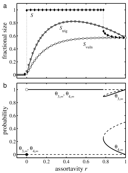
Figure 1: (a) Three key spreading measures as a function of assortativity $r$ for networks with $P_{k}=\frac{4}{7}\delta_{k3}+\frac{3}{7}\delta_{k4}$. Solid lines indicate theoretical curves and symbols represent measurements from simulations. The three curves are (1) the fractional size of the largest vulnerable component, $S_{\rm vuln}$, (Eq. (35), circles); (2) the fractional size of the largest triggering component, $S_{\rm trig}$, (Eq. (37), squares); and (3) the fractional size of global spreading events $S$ (Eq. (22), diamonds). The upper discontinuous phase transition in $S$ occurs at $r=r_{c}^{\rm upper}=0.77485\pm 0.00001$. The data shown were obtained from networks with $N$=0.98$\times 10^{5}$ nodes (correlations were generated using a shuffling algorithm described in Payne and Eppstein (2008)) with initial seeds placed at each node of 10 sample networks for a total of 9.8$\times 10^{5}$ samples per each value of $r$. (b) Solutions for $\theta_{3,\infty}$ and $\theta_{4,\infty}$, the probability that edges leading to degree 3 and 4 nodes will be from nodes in state $\sigma_{1}$ in the long time limit (see Eqs. (38) and (39).) Solid and dashed lines indicate stable and unstable ones respectively. When $r$ reaches $r_{c}^{\rm upper}$, a repeated solution appears for $(\theta_{3,\infty},\theta_{4,\infty})$, distinct from $(1,1)$, giving rise to the discontinuous upper phase transition in $S$.

As shown in Fig. 1(a), we obtain excellent agreement between equations and the output of simulations for $k_{b}=4$ on networks with $N=0.98\times 10^{5}$ nodes and $\tau=1/3$. We used this particular value of $N$ since it is the nearest number to $10^{5}$ that is divisible by $7$ [required by Eqs. (24) and (25)] and, for convenience, also a multiple of 100. As was observed for the original threshold model on random networks (Watts, 2002), we find that well-connected networks near the transition to a non-percolating largest vulnerable component are of a ‘robust-yet-fragile’ nature (Carlson and Doyle, 2000). We see in Fig. 1(a) that if assortativity $r$ is just slightly positive, and if the initial seed is in the small triggering component present, then spreading reaches the entire network. These otherwise highly resilient networks have an Achilles heel that leads to a complete transition in individual node states. Furthermore, finite size effects may be significant: for the networks with $N=9800$ nodes, our simulations show that global spreading is possible for $r$ as low as $-0.07$.

While our expressions for $S_{\rm vuln}$ and $S_{\rm trig}$ only depend coarsely on $\vec{b}_{1}$, the final extent of a global spreading event $S$ is more sensitive to changes in node response functions. Taking as an example one of our bimodal networks with $k_{a}=3$ and $k_{b}=10$, we see any value of $\tau$ in $(\frac{1}{10},\frac{1}{3}]$ is equivalent to $\tau=\frac{1}{3}$, as far as $S_{\rm vuln}$ and $S_{\rm trig}$ are concerned, since only degree 3 nodes are vulnerable. However, whether or not degree 10 nodes are vulnerable to $i$ neighbors switching to state $\sigma_{1}$ depends on $\tau$ meeting and exceeding $\frac{i}{10}$. For the case $k_{a}=3$ and $k_{b}=4$, the results we present here apply for all $\tau$ in $(\frac{1}{4},\frac{1}{3}]$.

For the final size of global spreading events, $S$, manipulations of Eq. (II) for $k_{a}=3$ and $k_{b}=4$ show we need to solve the following for $\theta_{3,\infty}$:

$$\theta_{3,\infty}=\frac{1+r}{2}i(2-\theta_{3,\infty})\theta_{3,\infty}+\frac{1-r}{2}(3-\theta_{4,\infty})\theta_{4,\infty}^{2}$$ (38)

where

$$\theta_{4,\infty}=\frac{1}{1-r}\theta_{3,\infty}(1-3r+2r\theta_{3,\infty})$$ (39)

for $0\leq r<1$. Knowing that $\theta_{3,\infty}=1$ is a solution of Eq. (38) means we can reduce the problem to solving for the roots of a quartic, for which we could obtain a complete analytic solution. For our purposes, numerical simulation is sufficient.

Our simulations and numerical analyses indicate the presence of another kind of phase transition in $S$. At the upper limit of $r=1$, the network is separated into two giant, fully-connected components, one comprising solely $k=3$ degree nodes and the other $k=4$ degree nodes (the giant component is of fractional size 1 for all other values of $r$). Spreading therefore occurs only in the $k=3$ degree node component when $r=1$, and, as shown in Fig. 1(a), the three quantities $S$, $S_{\rm vuln}$, and $S_{\rm trig}$ all equal 4/7 for complete assortativity.

As we decrease $r$ however, the possibility that a degree $k=4$ node is connected to two (or more) degree $k=3$ nodes in the giant vulnerable component increases. The expected size $\phi_{\infty}$ of a global spreading event grows gradually until it reaches a discontinuous phase transition and $\phi_{\infty}$ jumps to 1. Through numerical analysis of Eq. (38), we see that as $r$ increases, a repeated root $\theta_{3,\infty}$ appears when $r=r_{c}^{\rm upper}\simeq 0.775$. The roots become real and separate with both of them limiting to 1 as $r\rightarrow 1$. Fig. 1(b) shows how both $\theta_{3,\infty}$ and $\theta_{4,\infty}$ behave as a function of $r$. Note that the discontinuity in the final size of a global spreading event is not reflected in the curves for $S_{\rm trig}$ or $S_{\rm vuln}$, which both change smoothly for $0\leq r\leq 1$.

IV Concluding remarks

We have developed a series of theoretical expressions for a general class of spreading models on random networks with tunable degree assortativity $r$. Our main results are the derivation of the fractional size of the giant vulnerable and triggering components as a function of degree-degree distribution $e_{jk}$. When we allow all nodes to be susceptible with uniform probability $b$, our results reduce to the standard disease-like spreading case, and when we further set $b=1$, we obtain the conditions for the existence of a giant component.

When we set $r=0$, we also retrieve the condition for the existence of a giant vulnerable component (Eq. (12)) along with its size (Eq. (II)) in pure random networks with arbitrary degree distributions (Watts, 2002). For the triggering component, aside from our work for general $r$, we have also added to known results for the $r=0$ case. We have obtained the probability that an exogenously activated node of degree $k$ may trigger a global spreading event (Eq. (18)) and hence the probability that a randomly chosen node may do the same (Eq. (II)). Our work complements the results of Gleeson (Gleeson, 2008) which determines the final size of a global spreading event (Eqs. (22) and (II)). We note that a basic description of many kinds of spreading from a single initial seed must separately report (1) the probability of a global spreading event $P_{\rm trig}$, and (2) the expected final size $S$. The distribution of final sizes is often bimodal and an overall expected size conflates $P_{\rm trig}$ and $S$ in a potentially misleading way, since no size other than 0 and $S$ are in fact possible. Finally, the simple family of random networks we have considered here with $P_{k}=\frac{4}{7}\delta_{k3}+\frac{3}{7}\delta_{k4}$ have allowed us to demonstrate, for one example, the validity of our theoretical results for $S_{\rm vuln}(r)$ and $S_{\rm trig}(r)$.

Appendix: Calculations regarding collapse of general global spreading condition for uncorrelated networks

In the main text, we noted that the general condition for global spreading, that $\left|\mathbf{A}_{\mathbf{E},\vec{b}_{1}}\right|=0$ (Eq. (12)), collapses to the appropriate condition for uncorrelated networks when we set $e_{jk}=q_{j}q_{k}$ (Eq. (13)). We demonstrate this in two distinct ways. First, we take a direct route by setting $e_{jk}=q_{j}q_{k}$ in the definition of $\mathbf{A}_{\mathbf{E},\vec{b}_{1}}$:

$$\left[\mathbf{A}_{\mathbf{E},\vec{b}_{1}}\right]_{j+1,k+1} = \delta_{jk}q_{k}-kb_{k+1,1}q_{j}q_{k}$$ (40)

$$= \left(\delta_{jk}-q_{j}kb_{k+1,1}\right)q_{k}.$$

The $q_{k}$ that has been factored out stands as a multiple for the $k$th column, and therefore, by multilinearity of determinants (Strang, 2009), contributes to the determinant of $\mathbf{A}_{\mathbf{E},\vec{b}_{1}}$ as a simple overall multiplicative factor. In finding $|\mathbf{A}_{\mathbf{E},\vec{b}_{1}}|$, we can therefore focus on the matrix $[\delta_{jk}-q_{j}kb_{k+1,1}].$ We find the determinant of this matrix by finding its eigenvalues, which are the eigenvalues of $[-q_{j}kb_{k+1,1}]$ incremented by 1 due to the addition of the identity matrix. Since $[-q_{j}kb_{k+1,1}]$ is an outer product of the two vectors $[-q_{j}]$ and $[kb_{k+1,1}]$, we have a rank one matrix which therefore has a sole non-zero eigenvalue corresponding to an eigenvector in the direction of $[-q_{j}]$. We find the non-zero eigenvalue by explicitly applying the matrix $[-q_{j}kb_{k+1,1}]$ to $[-q_{j}]$, giving us $\lambda_{1}=-\sum_{k=0}^{\infty}kb_{k+1,1}q_{k}$. Shifting the summation index, we have $\lambda_{1}=-\sum_{k=1}^{\infty}(k-1)b_{k,1}q_{k-1}$, and $\lambda_{i}=0$ for $i\geq 2$. We now add 1 to all eigenvalues to obtain $\lambda_{1}^{\prime}=1-\sum_{k=1}^{\infty}(k-1)b_{k,1}q_{k-1}$ and $\lambda_{i}^{\prime}=1$ for $i\geq 2$. The determinant of $\mathbf{A}_{\mathbf{E},\vec{b}_{1}}$ is given by the product of the $\lambda_{i}^{\prime}$ along with the product of the $q_{k}$ elements we initially factored out:

$$|\mathbf{A}_{\mathbf{E},\vec{b}_{1}}|=\left(\prod_{k=0}^{\infty}q_{k}\right)\left(1-\sum_{k=1}^{\infty}(k-1)b_{k,1}q_{k-1}\right).$$ (41)

Since the $q_{k}$ are not equal to 0, the condition that $|\mathbf{A}_{\mathbf{E},\vec{b}_{1}}|=0$ for uncorrelated networks depends on the second term: $0=1-\sum_{k=1}^{\infty}b_{k,1}(k-1)q_{k-1}$. Substituting $q_{k}=kp_{k}/k_{\rm avg}$ gives us the desired condition of Eq. (13).

Secondly, we can also show that $F_{k}^{\prime}(1;\vec{b}_{1})$ is independent of $k$, meaning that the expected size of a finite subcomponent found at the other end of an edge connected to a node of degree $k+1$ does not depend on the latter’s degree. This will also lead us to the same condition for global spreading we found above. To do so, we return to Eq. (6) and set $e_{jk}=q_{j}q_{k}$:

$$\sum_{k=0}^{\infty}\left(\delta_{jk}q_{k}-kb_{k+1,1}q_{j}q_{k}\right)F_{k}^{\prime}(1;\vec{b}_{1})=\sum_{k=0}^{\infty}q_{j}q_{k}b_{k+1,1}.$$ (42)

Breaking the left hand side into two pieces, carrying out the first summation, and then dividing through by $q_{j}$, we obtain

$$F_{j}^{\prime}(1;\vec{b}_{1})-\sum_{k=0}^{\infty}kb_{k+1,1}q_{k}F_{k}^{\prime}(1;\vec{b}_{1})=\sum_{k=0}^{\infty}q_{k}b_{k+1,1}.$$ (43)

Upon rearranging, we can now express $F_{j}^{\prime}(1;\vec{b}_{1})$ as a function of terms not involving $j$ (even if they include summations involving $F_{k}^{\prime}(1;\vec{b}_{1})$), thereby demonstrating independence:

$$F_{j}^{\prime}(1;\vec{b}_{1})=\sum_{k=0}^{\infty}kb_{k+1,1}q_{k}F_{k}^{\prime}(1;\vec{b}_{1})+\sum_{k=0}^{\infty}q_{k}b_{k+1,1}.$$ (44)

Setting $F_{k}^{\prime}(1;\vec{b}_{1})=F^{\prime}(1;\vec{b}_{1})$ for all $k$, the above is now solvable, and we find

$$F^{\prime}(1;\vec{b}_{1})=\frac{\sum_{k=0}^{\infty}q_{k}b_{k+1,1}.}{1-\sum_{k=0}^{\infty}kb_{k+1,1}q_{k}}.$$ (45)

Finally, we see that setting the denominator to 0 recovers the condition for global spreading in uncorrelated networks.

References

- Newman (2003a) M. E. J. Newman, SIAM Review 45, 167 (2003a).
- Boccaletti et al. (2006) S. Boccaletti, V. Latora, Y. Moreno, M. Chavez, and D.-U. Hwang, Physics Reports 424, 175 (2006).
- Coleman et al. (1966) J. Coleman, H. Menzel, and E. Katz, Medical Innovations: A Diffusion Study (Bobbs Merrill, New York, 1966).
- Hatfield et al. (1993) E. Hatfield, J. T. Cacioppo, and R. L. Rapson, Emotional Contagion, Studies in Emotion and Social Interaction (Cambridge University Press, Cambridge, UK, 1993).
- Fowler and Christakis (2008) J. H. Fowler and N. A. Christakis, BMJ 337, article #2338 (2008).
- Murray (2002) J. D. Murray, Mathematical Biology (Springer, New York, 2002), Third ed.
- Anderson and May (1991) R. M. Anderson and R. M. May, Infectious Diseases of Humans: Dynamics and Control (Oxford Univ. Press, Oxford, 1991).
- Sachtjen et al. (2000) M. L. Sachtjen, B. A. Carreras, and V. E. Lynch, Phys. Rev. E 61, 4877 (2000).
- Kinney et al. (2005) R. Kinney, P. Crucitti, R. Albert, and V. Latora, Eur. Phys. J. B 46, 101 (2005).
- Newman et al. (2002) M. E. J. Newman, S. Forrest, and J. Balthrop, Phys. Rev. E 66, 035101 (2002).
- Balthrop et al. (2004) J. Balthrop, S. Forrest, M. Newman, and M. W. Williamson, Science 304, 527 (2004).
- Sornette (2003) D. Sornette, Why Stock Markets Crash: Critical Events in Complex Financial Systems (Princeton University Press, Princeton, NJ, 2003).
- Watts (2002) D. J. Watts, Proc. Natl. Acad. Sci. 99, 5766 (2002).
- Schelling (1971) T. Schelling, J. Math. Sociol. 1, 143 (1971).
- Schelling (1978) T. C. Schelling, Micromotives and Macrobehavior (Norton, New York, 1978).
- Granovetter (1978) M. Granovetter, Am. J. Sociol. 83, 1420 (1978).
- Stauffer and Aharony (1992) D. Stauffer and A. Aharony, Introduction to Percolation Theory (Taylor & Francis, Washington, D.C., 1992), Second ed.
- Newman et al. (2001) M. E. J. Newman, S. H. Strogatz, and D. J. Watts, Phys. Rev. E 64, 026118 (2001).
- Gleeson and Cahalane (2007) J. P. Gleeson and D. J. Cahalane, Phys. Rev. E 75, 056103 (2007).
- Gleeson (2008) J. P. Gleeson, Phys. Rev. E 77, 046117 (2008).
- Newman (2002) M. Newman, Phys. Rev. Lett. 89, 208701 (2002).
- Newman (2003b) M. E. J. Newman, Phys. Rev. E 67, 026126 (2003b).
- (23) The composition rule applies for a sum of identical random variables where the number summed is itself a random variable (the emanating degree in our particular case). Specifically, if we have two non-negative integer variables and with probabilities and , and generate a third random variable as , then where is the generating function for .
- Diekmann et al. (1998) O. Diekmann, M. C. M. De Jong, and J. A. J. Metz, J. Appl. Prob. 35, 448 (1998).
- Payne and Eppstein (2008) J. L. Payne and M. J. Eppstein, in Proceedings of the Genetic and Evolutionary Computation Conference, edited by M. Keijzer et al. (2008), p. 241.
- Carlson and Doyle (2000) J. Carlson and J. Doyle, Phys. Rev. Lett. 84, 2529 (2000).
- Strang (2009) G. Strang, Introduction to Linear Algebra (Cambridge Wellesley Press, Wellesley, MA, 2009), 4th ed.