Factorization of low-energy gluons in exclusive processes

Abstract

We outline a proof of factorization in exclusive processes, taking into account the presence of soft and collinear modes of arbitrarily low energy, which arise when the external lines of the process are taken on shell. Specifically, we examine the process of $e^{+}e^{-}$ annihilation through a virtual photon into two light mesons. In an intermediate step, we establish a factorized form that contains a soft function that is free of collinear divergences. In contrast, in soft-collinear effective theory, the low-energy collinear modes factor most straightforwardly into the soft function. We point out that the cancellation of the soft function, which relies on the color-singlet nature of the external hadrons, fails when the soft function contains low-energy collinear modes.

I Introduction

Factorization theorems are fundamental to modern calculations in QCD of the amplitudes for hard-scattering exclusive hadronic processes. They allow one to separate contributions to the amplitudes that involve states of high virtuality from those that involve states of low virtuality. The former, short-distance contributions can, by virtue of asymptotic freedom, be calculated in perturbation theory, while the latter, long-distance contributions are parametrized in terms of inherently nonperturbative matrix elements of QCD operators in hadronic states.

States of low virtuality can arise from the emission of a soft gluon, whose four-momentum components are all small, or from the emission of a collinear gluon, whose four-momentum is nearly parallel to the four-momentum of a gluon or light quark. In some discussions of factorization that employ soft-collinear effective theory (SCET) Bauer:2000yr ; Bauer:2001yt ; Bauer:2002nz or diagrammatic methods Bodwin:2008nf , it is assumed that gluons can have no transverse momentum components that are smaller than the QCD scale $\Lambda_{\rm QCD}$. That is, gluons can have hard momentum, in which all components are of order the hard-scattering scale $Q$, soft momentum, in which all components are of order $\Lambda_{\rm QCD}$, or collinear momentum, in which the transverse components are of order $\Lambda_{\rm QCD}$ and the energy and longitudinal spatial component are much larger than $\Lambda_{\rm QCD}$ (usually taken to be of order $Q$). This assumption is appropriate to the discussion of physical hadrons, in which confinement provides a nonperturbative IR cutoff of order $\Lambda_{\rm QCD}$. However, in perturbative matching calculations of short-distance coefficients, one usually takes the external quark and gluon states to be on their mass shells, and, in this situation, soft and collinear gluons of arbitrarily low energy can be emitted. In order to establish the consistency of such calculations, one must prove, to all orders in perturbation theory, that these soft and collinear gluons factor from the hard-scattering process and that the factorized form is identical to the conventional one that is obtained in the presence of an infrared cutoff of order $\Lambda_{\rm QCD}$. In the absence of such a proof, one would have no guarantee in the matching calculation that low-virtuality soft and collinear contributions either cancel or can be absorbed entirely into the standard nonperturbative functions (distribution functions in inclusive processes and distribution amplitudes in exclusive processes).

At the one-loop level, gluons of arbitrarily low energy can be treated along with higher-energy soft and collinear gluons, and the conventional proofs of factorization apply. However, as we shall see, the proof of factorization of low-energy gluons becomes more complicated beyond one loop. In multiloop integrals, in the on-shell case, one finds contributions at leading power in the hard-scattering momentum in which collinear gluons of low energy couple to soft gluons. Our goal is to construct a proof of factorization that takes this possibility into account. To our knowledge, the existing discussions of factorization, either in the context of SCET or diagrammatic methods, have not addressed this possibility.

In on-shell perturbative calculations in SCET, gluon transverse momenta extend to zero. Hence, the possibility of low-energy gluons with momenta collinear to one of the external particles arises. At one-loop level, the soft and collinear contributions can be separated through the use of an additional cutoff Manohar:2006nz . However, as we have already mentioned, at two-loop level and higher, a low-energy collinear gluon can attach to a soft gluon. The SCET action is formulated so that soft gluons can be decoupled from collinear gluons through a field redefinition, but there is no corresponding provision to decouple collinear gluons from soft gluons. Therefore, it seems that, in SCET, low-energy collinear gluons would be treated most straightforwardly as part of the soft (or ultrasoft) contribution. This results in a factorized form in which the soft function contains gluons with both soft and collinear momenta and, hence, contains both soft and collinear divergences.

Alternatively, one can consider a factorized form in which gluons with collinear momenta are factored completely from the soft function, so that they reside only in jet functions that are associated with the initial- or final-state hadrons. Such an alternative factorized form, in which the soft function is free of collinear divergences, has been discussed in the context of factorization for the Drell-Yan process in Refs. Bodwin:1984hc ; Collins:1985ue ; Collins:1989gx , although the details of the factorization of gluons with collinear momenta from the soft function were not given. This alternative factorized form has also been discussed in connection with resummation of logarithms in, for example, Refs. Collins:1984ik ; Sterman:1986aj ; Contopanagos:1996nh ; Kidonakis:1998bk ; Kidonakis:1998nf ; Sterman:2002qn . Furthermore, it has been discussed in an axial gauge in the context of on-shell quark scattering Sen:1982bt . Axial gauges are somewhat problematic, in that they introduce unphysical singularities into gluon and ghost propagators. Such singularities could potentially spoil contour-deformation arguments that are used to ascertain the leading regions of integration in Feynman diagrams Collins:1982wa . For this reason, we believe that it is important to construct a proof of factorization in a covariant gauge, such as the Feynman gauge, which we employ in the present paper.

A factorized form in which the soft function contains no gluons with collinear momenta has several useful features. One is that contributions in which there are two logarithms per loop (one collinear and one soft) reside entirely in the jet functions, which have a diagonal color structure, rather than in the soft function, which has a more complicated color structure. Here we focus on a feature that is crucial for factorization proofs: A factorized form in which the soft function contains no collinear modes allows one to establish a cancellation of the soft function when it connects to a color-singlet hadron. As we shall explain below, if the soft function contains gluons with collinear momenta, then the cancellation of the soft function fails at leading order in the large momentum scale.

In this paper, we outline the proof of factorization at leading order in the hard-scattering momentum for the case of on-shell external partons. For concreteness, we discuss the example of the exclusive production of two light mesons in $e^{+}e^{-}$ annihilation. In an intermediate step, the factorized form that we obtain contains a soft function that is free of collinear divergences. This allows us to demonstrate the cancellation of the soft function at leading order in the large momentum scale. Our proof makes use of standard all-orders diagrammatic methods for proving factorization Bodwin:1984hc ; Collins:1985ue ; Collins:1989gx . We find that the factorization of gluons of arbitrarily low energy can be dealt with conveniently by focusing on the factorization of contributions to loop integrals from singular regions, i.e., regions that contain the soft and collinear singularities. Such singular regions are discussed in Refs. Collins:1985ue ; Collins:1989gx . However, the coupling of low-energy collinear gluons to soft gluons is not discussed in those papers.

The remainder of this paper is organized as follows. In Sec. II we describe the model that we use for the production amplitude. Section III contains a heuristic discussion of the regions of loop momenta that give leading contributions. This discussion is aimed at making contact with previous work on factorization and also sets the stage for a more precise discussion of the singular regions of loop momenta. In Sec. IV, we discuss the diagrammatic topology of the leading contributions and also the topology of the soft and collinear singular contributions. We treat the collinear and soft contributions by making use of collinear and soft approximations that are valid in the singular regions. These are discussed in Sec. V, along with the decoupling relations for the collinear and soft singular contributions. In Sec. VI, we outline the factorization of the collinear and soft singularities and describe how one arrives at the standard factorized form for the production amplitude. We also outline the proof of factorization in the case in which the relative momentum between the quark and the antiquark in a meson is taken to be nonzero. Here, we discuss the difficulty that arises in the cancellation of the soft function if the soft function contains gluons with collinear momenta. Finally, in Sec. VII, we summarize our results.

II Model for the amplitude

Let us consider the exclusive production of two light mesons in $e^{+}e^{-}$ annihilation through a single virtual photon. We work in the $e^{+}e^{-}$ center-of-momentum frame and in the Feynman gauge, and we write four-vectors in terms of light-cone components: $k=(k^{+},k^{-},\bm{k}_{\perp})$, with $k^{\pm}=(1/\sqrt{2})(k^{0}\pm k^{3})$. We take each meson to be moving in the plus (minus) direction and to consist of an on-shell quark with momentum $p_{1q}$ ($p_{2q}$) and an on-shell antiquark with momentum $p_{1\bar{q}}$ ($p_{2\bar{q}}$):

$$p_{1q} = \left[\frac{z_{1}Q}{\sqrt{2}},\frac{\bm{p}_{1\perp}^{2}}{\sqrt{2}z_{1}Q},\bm{p}_{1\perp}\right],$$ (1a)

$$p_{1\bar{q}} = \left[\frac{(1-z_{1})Q}{\sqrt{2}},\frac{\bm{p}_{1\perp}^{2}}{\sqrt{2}(1-z_{1})Q},-\bm{p}_{1\perp}\right],$$ (1b)

$$p_{2q} = \left[\frac{\bm{p}_{2\perp}^{2}}{\sqrt{2}z_{2}Q},\frac{z_{2}Q}{\sqrt{2}},\bm{p}_{2\perp}\right],$$ (1c)

$$p_{2\bar{q}} = \left[\frac{\bm{p}_{2\perp}^{2}}{\sqrt{2}(1-z_{2})Q},\frac{(1-z_{2})Q}{\sqrt{2}},-\bm{p}_{2\perp}\right],$$ (1d)

where $0<z_{i}<1$ and $z_{i}$ does not lie near the endpoints of its range. The momentum $P_{i}$ of the meson $M_{i}$ is given by

$$P_{i}=p_{iq}+p_{i\bar{q}}.$$ (2)

The large scale $Q$ is equal to the invariant mass of the virtual photon, up to corrections of relative order $\bm{p}_{i\perp}/Q$. We assume that the components of $\bm{p}_{i\perp}$ are all of order $\Lambda_{\rm QCD}$. It is useful for subsequent discussions to introduce a dimensionless parameter

$$\lambda\equiv\Lambda_{\rm QCD}/Q.$$ (3)

In order to simplify the initial discussion, we set $\bm{p}_{i\perp}=0$. We will discuss at the end of the factorization argument the effect of keeping the $\bm{p}_{i\perp}$ nonzero.

III Leading regions of loop momenta

Let us now discuss the regions of loop momenta that are leading in powers of the large scale $Q$. Our analysis will be somewhat heuristic, in that, as we will see, the boundaries between the various momentum types are indistinct. We carry out this analysis in order to make contact with previous discussions of factorization and to set the stage for our proof of factorization. That proof focuses on the soft and collinear singular regions of loop momenta, which are distinct.

Suppose that a virtual gluon with momentum $k$ attaches to external $q$ or $\bar{q}$ lines with momentum $p_{i}$ and $p_{j}$. (In the remainder of this paper, we call lines that originate in an external $q$ or $\bar{q}$ “outgoing fermion lines.”) In the limit in which the components of $k$ are all small compared to the largest components of $p_{i}$ and $p_{j}$, the amplitude associated with this process is proportional to

$$\int d^{4}k\frac{4p_{i}\cdot p_{j}}{(2p_{i}\cdot k+i\varepsilon)(-2p_{j}\cdot k+i\varepsilon)}\frac{1}{k^{2}+i\varepsilon}.$$ (4)

Because the integral is independent of the scale of $k$, leading contributions arise from arbitrarily small momentum $k$. One can emit an additional virtual gluon of momentum $k^{\prime}$ from an outgoing fermion line at a point to the interior of the emission of a gluon with momentum $k$, provided that $k^{\prime}\cdot p_{i}\gtrsim k\cdot p_{i}$. Such emissions are arranged in a hierarchy along the outgoing fermion lines, according to the virtualities that the emissions produce on the outgoing fermion lines.

Now let us establish some nomenclature to describe the regions of loop momenta that yield contributions that are leading in powers of the large scale $Q$. We call such momentum regions “leading regions.” We outline below the construction of an argument to prove that these are the only possible leading regions. We consider hard ($H$), soft ($S$), collinear-to-plus ($C^{+}$), and collinear-to-minus ($C^{-}$) momenta, whose components have the following orders of magnitude:

$$H\,\,\, Q(1,1,\bm{1}_{\perp}),$$ : (5a)

$$S\,\,\,\, Q\epsilon_{S}(1,1,\bm{1}_{\perp}),$$ : (5b)

$$C^{+} Q\epsilon^{+}[1,(\eta^{+})^{2},\bm{\eta}^{+}_{\perp}],$$ : (5c)

$$C^{-} Q\epsilon^{-}[(\eta^{-})^{2},1,\bm{\eta}^{-}_{\perp}].$$ : (5d)

We call a line in a Feynman diagram that carries momentum of type $X$ an “$X$ line.” The parameters $\epsilon_{S}$, $\epsilon^{+}$, and $\epsilon^{-}$ set the energy scales of the momenta. We define the soft region of momentum space by the condition

$$\epsilon_{S}\ll 1.$$ (6)

We define the collinear region of momentum space by the conditions

$$\epsilon^{\pm} \lesssim 1,$$

$$\eta^{\pm} \ll 1.$$ (7)

In our definitions of momentum regions, the positions of the boundaries between regions are somewhat vague. That is because there is no clear distinction between the $H$, $S$, and $C^{\pm}$ regions near the boundaries between regions: When $\epsilon_{S}\sim 1$, an $S$ momentum is essentially an $H$ momentum; when $\eta^{\pm}\sim 1$, a $C^{\pm}$ momentum is essentially an $S$ momentum.

Soft singularities occur in the limit $\epsilon_{S}\to 0$, and $C^{\pm}$ singularities occur in the limits $\eta^{\pm}\to 0$. Hence, we see that, unlike the soft and collinear momentum regions, the soft and collinear singularities are distinct. There are also singularities that are associated with the scales of the collinear momenta. These appear in the limit $\epsilon^{\pm}\to 0$. If $\eta^{\pm}$ is finite, these are essentially soft singularities, but they can occur in conjunction with a collinear singularity if $\eta^{\pm}\to 0$.

We do not consider gluon loop momenta of the “Glauber” type Bodwin:1981fv , in which $k^{+},k^{-}\ll|\bm{k}_{\perp}|$. The reason for this is that, for exclusive processes, the $k^{+}$ and $k^{-}$ contours of integration are not pinched in the Glauber region, and, hence, one can always deform them out of that region Collins:1982wa .

If we take $\epsilon^{\pm}$ to be of order one and $\epsilon_{S}$ and $\eta^{\pm}$ to be of order $\lambda$ [Eq. (3)], then the resulting momenta are those that are treated in SCET_II Bauer:2002aj . Soft momenta with $\epsilon_{S}$ of order $\lambda^{2}$ have been considered in Ref. Beneke:2000ry in the context of two-loop-order contributions to $B$-meson decays, and the possibility of leading momentum regions involving momenta of arbitrarily small energy is mentioned in Ref. Smirnov:1999bza for the case of massive particles.

$k$ $\backslash$ $p$          $S$           $C^{\pm}$           $\tilde{C}^{\pm}$    $S$ $\epsilon_{S_{k}}\sim\epsilon_{S_{p}}$ $\epsilon_{p}^{\pm}(\eta^{\pm}_{p})^{2}\lesssim\epsilon_{S_{k}}\ll\epsilon_{p}^{\pm}$ $\epsilon_{p}^{\pm}\tilde{\eta}^{\pm}_{p}\lesssim\epsilon_{S_{k}}\ll\epsilon_{p}^{\pm}$

$k$ $\backslash$ $p$          $S$          $C^{\mp}$          $\tilde{C}^{\mp}$          $CC$    $C^{\pm}$ $\epsilon^{\pm}_{k}\sim\epsilon_{S_{p}}$ $\epsilon_{p}^{\mp}(\eta^{\mp}_{p})^{2}\lesssim\epsilon^{\pm}_{k}\lesssim\epsilon^{\mp}_{p}$ $\epsilon^{\mp}_{p}\tilde{\eta}^{\mp}_{p}\lesssim\epsilon^{\pm}_{k}\lesssim\epsilon^{\mp}_{p}$ $\epsilon^{\pm}_{k}\sim\epsilon_{{CC}_{p}}$ $CC$ $\epsilon_{CC_{k}}\sim\epsilon_{S_{p}}$ $\epsilon_{p}^{\mp}(\eta^{\mp}_{p})^{2}\lesssim\epsilon_{CC_{k}}\ll\epsilon^{\mp}_{p}$ $\epsilon^{\mp}_{p}\tilde{\eta}^{\mp}_{p}\lesssim\epsilon_{CC_{k}}\ll\epsilon^{\mp}_{p}$ $\epsilon_{CC_{k}}\sim\epsilon_{CC_{p}}$

Table 1: Conditions under which a gluon with momentum $k$ can attach to a line with momentum $p$. In each table, the left-hand column gives the momentum type of the gluon with momentum $k$, and the top row gives the momentum type of the line with momentum $p$. Each entry gives the conditions that must be fulfilled if the attachment is to satisfy our conventions for attachments, as described in the text, and also yield a contribution that is not suppressed by powers of ratios of momentum components. For purposes of power counting, an $H$ line behaves as a soft line with $\epsilon_{S}\sim 1$. The rules for the attachment if $k$ is a $\tilde{C}^{\pm}$ momentum are the same as the rules of attachment if $k$ is a $C^{\pm}$ momentum. As is explained in the text, if $k$ is $S$, and the lines to which it attaches have momentum $p_{i}$ and $p_{j}$, then $p_{i}$ and $p_{j}$ cannot both be $C^{+}$ or $C^{-}$. Furthermore, if $k$ is $C^{\pm}$, then at least one of $p_{i}$ and $p_{j}$ is $C^{\pm}$.

We wish to determine the configurations of the various momentum types in a Feynman diagram that are leading, in the sense that they are not suppressed by powers of the ratios of momentum components. In our analysis, we begin with the hard subdiagram plus the bare external $q$ and $\bar{q}$ for each meson. Then we add one gluon at a time to the diagram. (Each added gluon possibly contains quark, gluon, and ghost vacuum polarization loops.) There are many redundant procedures for adding gluons to obtain a diagram with a given momentum configuration. We adopt the following convention: We say that a gluon with momentum $l$ can attach to a line with momentum $p$ only if the momentum $p+l$ is predominantly of the same type as momentum $p$. For example, an $S$ gluon with momentum $l$ can attach to a $C^{\pm}$ line with momentum $p$ only if $\epsilon_{S}$ is of order $\epsilon^{\pm}\eta^{\pm}$ or smaller, so that the plus (minus) component of $p+l$ is the dominant component. Similarly, a $C^{\pm}$ gluon with momentum $l$ can attach to an $S$ gluon with momentum $p$ only if $\epsilon^{\pm}$ is of order $\epsilon_{S}$ or smaller, so that all components of $p+l$ are approximately equal. We call the sum of a $C^{\pm}$ momentum and an $S$ momentum with $\epsilon_{S}\sim\epsilon^{\pm}\eta^{\pm}$ a $\tilde{C}^{\pm}$ momentum. The sum of a $C^{\pm}$ momentum and a $C^{\mp}$ momenta with $\epsilon^{\pm}(\eta^{\pm})^{2}\ll\epsilon^{\mp}\ll\epsilon^{\pm}$ is also a $\tilde{C}^{\pm}$ momentum. We also allow the attachment of a $C^{\pm}$ momentum to a $C^{\mp}$ momentum with $\epsilon^{+}\sim\epsilon^{-}$, and, in this case, we call the sum of the $C^{+}$ momentum and $C^{-}$ momentum a $CC$ momentum. These combination momenta have the following orders of magnitude:

$$\tilde{C}^{+} Q\epsilon^{+}(1,\tilde{\eta}^{+},\bm{\eta}^{+}_{\perp}),$$ : (8a)

$$\tilde{C}^{-} Q\epsilon^{-}(\tilde{\eta}^{-},1,\bm{\eta}^{-}_{\perp}),$$ : (8b)

$$CC Q\epsilon_{CC}(1,1,\bm{\eta}_{CC\perp}),$$ : (8c)

where

$$1\gg\tilde{\eta}^{\pm}\gg(\eta^{\pm})^{2}.$$ (9)

In order to determine the momenta of attached gluons that can result in a leading power count, it is useful to consider the expression (4). In the first two factors in the denominator of the expression (4), terms of the form $p_{i}^{2}$ and $k^{2}$ have been dropped. Thus, the denominator of the expression (4) gives a lower bound on the order of magnitude of the exact denominator. Because of our convention for the allowed momentum types for $k$, the numerator $p_{i}\cdot p_{j}$ in the expression (4) gives the leading behavior unless $p_{i}$ and $p_{j}$ are both either $C^{+}$ or $C^{-}$. For such cases, we need to consider numerator factors $k^{2}$, $k\cdot p_{i}$, and $k\cdot p_{j}$, in addition to $p_{i}\cdot p_{j}$. Otherwise, we can use the expression (4) as it stands to obtain an upper bound on the magnitude of the factors that appear when one adds a gluon. The expression (4) has the useful property that it is independent of the scales of the momenta $k$, $p_{i}$, and $p_{j}$, and so it can be used to determine rules for the leading momentum configurations that are independent of the scales of the momenta. From these considerations, it is easy to see that $k$ must be $S$, $C^{+}$, or $C^{-}$ in order to obtain a leading power count. We regard these momentum types as primary, in the sense that the loop-integration variables correspond to these momenta. Other momentum types can arise when we add these primary types, following our convention above for allowed attachments. It follows that, if $k$ is $S$, then $p_{i}$ and $p_{j}$ cannot both be $C^{+}$ or $C^{-}$. It also follows that, if $k$ is $C^{\pm}$, then at least one of $p_{i}$ and $p_{j}$ is $C^{\pm}$.

If we restore the terms of the form $p_{i}^{2}$ and $k^{2}$ in the denominators of the expression (4), then there can be an additional suppression of the amplitude. In order to obtain a leading contribution, we must have

$$k\cdot p \gtrsim k^{2},$$

$$k\cdot p \gtrsim p^{2}.$$ (10)

Taking into account the additional conditions in Eq. (10), we obtain the rules for the leading contributions that are given in Table 1. In Table 1, the symbol “$\sim$” means that quantities have the same order of magnitude. In each expression in Table I, if the quantity with subscript $k$ is much greater than the quantity with subscript $p$, then the attachment is not allowed because $p+k$ is not essentially of the same momentum type as $p$. If the quantity with subscript $k$ is much less than the quantity with subscript $p$, then the contribution is suppressed by a power of the ratio of those quantities. The rules in Table 1 also apply when the added gluon attaches to one of the outgoing fermion lines. In that case, one sets $\eta^{+}=0$ or $\eta^{-}=0$ on the outgoing fermion line. In Table 1, we have not given the rules for the attachments of gluons with $C^{\pm}$ or $\tilde{C}^{\pm}$ momenta to lines with $C^{\pm}$ or $\tilde{C}^{\pm}$ momenta. The rules for such attachments are complicated and cannot be characterized simply in terms of the magnitudes of the momentum components, as is the case for the attachments listed in Table  1. For our purposes, it suffices to note that necessary conditions for such attachments are given in Eq. (10).

The constraints in Eq. (10) imply that an attachment of a gluon to a given line is allowed only if the virtuality that it produces on that line is of order or greater than the virtuality that is produced by the gluons that attach to that line to the outside of the attachment in question. Here, and throughout this paper, “outside” means toward the on-shell ends of the external quark and antiquark lines. If a gluon with momentum $k$ of type $C^{\pm}$, $\tilde{C}^{\pm}$, $S$, $C^{\mp}$, or $CC$ attaches to a $C^{\pm}$ line from an on-shell outgoing quark or antiquark, it adds virtuality $Q^{2}\epsilon_{k}^{\pm}(\eta_{k}^{\pm})^{2}$, $Q^{2}\epsilon_{k}^{\pm}\tilde{\eta}_{k}^{\pm}$, $Q^{2}\epsilon_{S_{k}}$, $Q^{2}\epsilon_{k}^{\mp}$, or $Q^{2}\epsilon_{CC_{k}}$, respectively.

IV Topology of the leading contributions

IV.1 Topology of the leading momentum regions

By taking into account the allowed gluon attachments in Table 1, one arrives at the topology of Feynman diagrams that is shown in Fig. 1. This topology is similar in appearance to topologies that have been discussed previously in connection with the identification of IR (pinch) singularities in Feynman diagrams Sterman:1978bi ; Sterman:1978bj ; Libby:1978bx ; Collins:1989gx . However, as we will explain, the subdiagrams in Fig. 1 contain finite ranges of momenta, whereas those in Refs. Sterman:1978bi ; Sterman:1978bj ; Collins:1989gx contain only infinitesimal neighborhoods of the soft and collinear singularities. (We will discuss the topology of the soft and collinear singularities in Sec. IV.3.)

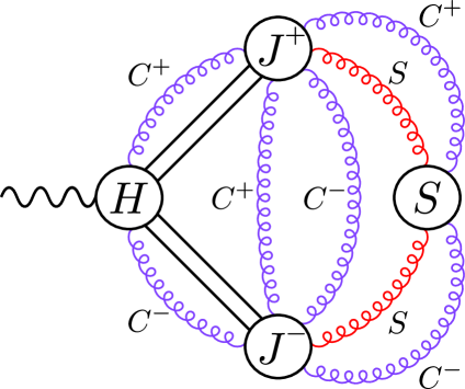
Figure 1: Leading regions for double light-meson production in $e^{+}e^{-}$ annihilation. The wavy line represents the virtual photon.

In the topology of Fig. 1, there is a jet subdiagram for each of the collinear regions (corresponding to each light meson), there is a hard subdiagram that includes the production process at lowest order in $\alpha_{s}$, and there is a soft subdiagram.

We include in the hard subdiagram all propagators that are off shell by order $Q^{2}$. That is, we include lines carrying both momentum $H$ and momentum $CC$ with $\epsilon_{CC}\sim 1$. (The propagators in the Born process carry momenta $CC$ with $\epsilon_{CC}\sim 1$.)

The soft subdiagram includes gluons with $S$ momenta, which may contain quark, gluon, and ghost loops. The soft subdiagram attaches to the jet subdiagrams through any number of $S$-gluon lines, according to the rules in Table 1. Note that a gluon carrying momentum $S_{i}$ cannot attach to a line carrying momentum $S_{j}$ unless $\epsilon_{S_{i}}\sim\epsilon_{S_{j}}$, and so various part of the soft subdiagram cannot attach to each other.

The $C^{\pm}$-jet subdiagram $J^{\pm}$ contains the external quark lines for the meson with $C^{\pm}$ momentum, as well as gluons with $C^{\pm}$ momenta, which may contain quark, gluon and ghost loops. We also include in $J^{\pm}$ lines carrying $CC$ momentum with $\epsilon_{CC}\ll 1$ that occur when a gluon carrying momentum $C^{\mp}$ from a $J^{\mp}$ jet attaches to a line carrying $C^{\pm}$ momentum in $J^{\pm}$. Each jet subdiagram attaches to the hard subdiagram through the external quark and antiquark lines and through any number of $C^{\pm}$ gluons with $\epsilon^{\pm}\sim 1$. A gluon carrying $C^{\pm}$ or $\tilde{C}^{\pm}$ momentum can connect the $J^{\pm}$ subdiagram to the $J^{\mp}$ subdiagram, but only with the attachments in Table 1. Of particular note is the fact that a gluon carrying momentum $C^{\pm}$ or $\tilde{C}^{\pm}$ can connect a $C^{\pm}$ jet to an $S$ line in the soft subdiagram, provided that $\epsilon^{\pm}\sim\epsilon_{S}$. This is a feature of scattering processes in the on-shell case that does not appear when one has an infrared cutoff of order $\Lambda_{\rm QCD}$. The factorization of gluons carrying collinear momenta from the soft subdiagram is one of the principal technical issues that we address in this paper.

In order to prove factorization, we need to show that the nonperturbative contributions to Feynman diagrams (those with virtualities of order $\Lambda_{\rm QCD}^{2}$ or less) either cancel or can be factored into the meson distribution amplitudes. Specifically, we will argue that the nonperturbative contributions associated with the soft divergences factor from the $J^{\pm}$ subdiagrams and cancel and that the nonperturbative contributions associated with the $C^{\pm}$ divergences factor from the $J^{\mp}$, hard, and soft subdiagrams and can be absorbed into the $J^{\pm}$ meson distribution amplitude. These factorizations and cancellations establish that the production amplitude depends only on the properties of the individual mesons, and not on correlations between the two mesons, except through the hard subprocess.

IV.2 Two-loop example

In Fig. 2 we show a two-loop example in which a $C^{+}$ gluon attaches to an $S$ gluon.

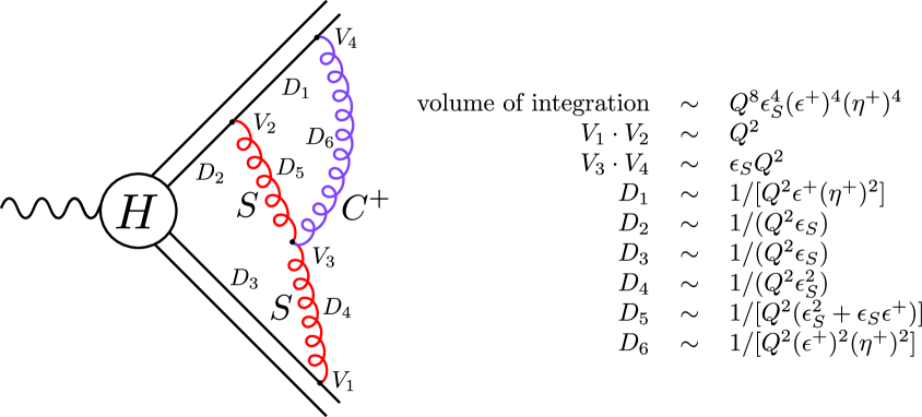
Figure 2: A two-loop example in which a $C^{+}$ gluon attaches to an $S$ gluon. The $V_{i}$ are the vertex factors, and the $D_{i}$ are the propagator factors.

We take the $C^{+}$ momentum to be $l_{1}=Q\epsilon^{+}(1,\eta^{2},\bm{\eta}^{+}_{\perp})$ and the $S$ momentum to be $l_{2}=Q\epsilon_{S}(1,1,\bm{1}_{\perp})$. We assume that $\epsilon^{+}\lesssim\epsilon_{S}$, and we route the $l_{1}$ momentum through the $D_{5}$ propagator. Then, we find the factors for the diagram that are shown on the right side of Fig. 2. Combining these factors, we obtain the following order of magnitude for the two-loop correction: $\epsilon_{S}\epsilon^{+}/(\epsilon_{S}^{2}+\epsilon_{S}\epsilon^{+})$. We see that this result is independent of $Q$, as expected, and is also independent of $\eta$. This contribution is leading if $\epsilon^{+}\sim\epsilon_{S}$, but it vanishes in the limit $\epsilon^{+}/\epsilon_{S}\to 0$, in accordance with the rule in Table 1.

IV.3 Topology of the singular momentum regions

In the preceding discussion, as we have noted, the soft and collinear momentum regions are not well distinguished. If $\eta^{\pm}\sim 1$, then a collinear momentum is virtually identical to a soft momentum. Similarly, if the components of a soft momentum have significantly different sizes, then a soft momentum can be virtually identical to a collinear momentum. In discussions of factorization, we rely on collinear approximations that are accurate only for $\eta^{\pm}\ll 1$. In order to apply such approximations, we must avoid the problems in distinguishing soft and collinear momenta that arise near the boundaries between these regions. Furthermore, the soft approximation for the attachment of a soft gluon to a $C^{\pm}$ line becomes inaccurate as the soft momentum becomes more nearly a $C^{\pm}$ momentum. Again, we encounter a problem that occurs near the boundary between momentum regions. In the discussion that follows, we avoid such boundary issues by focusing on infinitesimal neighborhoods of the soft and collinear singularities (singular regions). As a first step in proving factorization, we will demonstrate the factorization of these singular regions.

The topologies of soft and collinear singular regions have been discussed in the context of factorization theorems for inclusive processes in Refs. Collins:1985ue ; Collins:1989gx . These topologies follow from the rules for power counting that we have given in Sec. III. Let us describe the relationship of the topologies of the singular regions to the topologies in Fig. 1. The $C^{\pm}$ singularities reside in the outermost part of the $J^{\pm}$ subdiagram, which we call the $\tilde{J}^{\pm}$ subdiagram. (We consider the $\tilde{J}^{\pm}$ subdiagram to be part of the $J^{\pm}$ subdiagram, and we call the part of the $J^{\pm}$ subdiagram that excludes the $\tilde{J}^{\pm}$ subdiagram the $J^{\pm}-\tilde{J}^{\pm}$ subdiagram.) The soft singularities reside in the outermost part of the $S$ subdiagram, which we call the $\tilde{S}$ subdiagram. (We consider the $\tilde{S}$ subdiagram to be part of the $S$ subdiagram, and we call the part of the $S$ subdiagram that excludes the $\tilde{S}$ subdiagram the $S-\tilde{S}$ subdiagram.) $S$ singular gluons connect the $\tilde{S}$ subdiagram only to the $\tilde{J}^{\pm}$ subdiagrams. The $\tilde{J}^{\pm}$ subdiagrams connect to the $J^{\pm}$, $J^{\mp}$, $S$, and $H$ subdiagrams via $C^{\pm}$ gluons. We emphasize that the $\tilde{J}^{\pm}$ subdiagrams connect, via $C^{\pm}$ gluons to the $\tilde{S}$ subdiagram. This last type of connection is a feature that was not included in the discussion of leading (pinch) singularities in Refs. Collins:1985ue ; Collins:1989gx . Otherwise, the topologies that we find are the same as in Refs. Collins:1985ue ; Collins:1989gx , provided that we identify the hard subdiagram in those references with the union of all of the subdiagrams in our topology except for $\tilde{S}$, $\tilde{J}^{+}$, and $\tilde{J}^{-}$. We call this union $\tilde{H}$.

V Collinear and soft approximations and decoupling relations

Our strategy is to show that contributions from the $\tilde{J}^{\pm}$ subdiagrams factor from the $J^{\mp}$, hard, and $S$ subdiagrams and can be absorbed into the $J^{\pm}$ meson distribution amplitude and that contributions from the $\tilde{S}$ subdiagram factor from the $\tilde{J}^{\pm}$ subdiagrams and cancel. We treat the contributions from the $C^{\pm}$ singular regions by making use of a collinear-to-plus (minus) approximation Bodwin:1984hc ; Collins:1985ue ; Collins:1989gx for the $C^{\pm}$ gluons that attach the $\tilde{J}^{\pm}$ subdiagram to the $J^{\mp}$, $H$, and $\tilde{S}$ subdiagrams. The $C^{\pm}$ approximations capture all of the collinear-to-plus (minus) singularities, but become increasingly inaccurate as one moves away from the singularities. Similarly, we treat the contributions from the $S$ singular regions by using a soft approximation for the gluons with $S$ momentum that attach the $\tilde{S}$ subdiagram to the $\tilde{J}^{\pm}$ subdiagrams. The soft approximation captures all of the soft singularities, but becomes increasingly inaccurate as one moves away from the singularities.

V.1 Collinear approximation

Let us now describe the collinear approximation explicitly. Suppose that a gluon carrying momentum in the $C^{\pm}$ singular regions attaches to a line carrying $H$, $C^{\mp}$, $\tilde{C}^{\mp}$, $S$, or $CC$ momentum. Then, we can apply a collinear approximation to that gluon Bodwin:1984hc ; Collins:1985ue ; Collins:1989gx with no loss of accuracy. The collinear-to-plus ($C^{+}$) and collinear-to-minus ($C^{-}$) approximations consist of the following replacements in the gluon-propagator numerator:

$$g_{\mu\nu}\,\,\Longrightarrow\,\,\left\{\begin{array}[]{ll}\displaystyle\frac{k_{\mu}\bar{n}_{1\nu}}{k\cdot\bar{n}_{1}-i\varepsilon}&(C^{+}),\\[8.61108pt] \displaystyle\frac{k_{\mu}\bar{n}_{2\nu}}{k\cdot\bar{n}_{2}+i\varepsilon}&(C^{-}).\end{array}\right.$$ (11)

The index $\mu$ corresponds to the attachment of the gluon to the hard, soft, or $J^{\mp}$ subdiagram, and the index $\nu$ corresponds to the attachment of the gluon to the $J^{\pm}$ subdiagram. Our convention is that $k$ flows out of a $C^{+}$ line and into a $C^{-}$ line. There is considerable freedom in choosing the auxiliary vectors $\bar{n}_{1}$ and $\bar{n}_{2}$. In order to reproduce the amplitude in the collinear singular region, it is only necessary to have $\bar{n}_{1}\cdot p_{1q}>0$ (or $\bar{n}_{1}\cdot p_{1\bar{q}}>0$) and $\bar{n}_{2}\cdot p_{2q}>0$ (or $\bar{n}_{2}\cdot p_{2\bar{q}}>0$). We choose $\bar{n}_{1}$ and $\bar{n}_{2}$ to be lightlike vectors in the minus and plus directions such that, for any vector $q$, $q\cdot\bar{n}_{1}=q^{+}$ and $q\cdot\bar{n}_{2}=q^{-}$. The $C^{\pm}$ approximation relies on the fact that the $\pm$ component of $k$ dominates in the collinear limit, provided that the $\mu$ index connects to a current in which the $\mp$ component is nonzero. Because of this last stipulation, we cannot apply the collinear approximations to a gluon carrying momentum in the $C^{\pm}$ singular region when it attaches to a line that is also carrying momentum in the $C^{\pm}$ singular region. In the $C^{\pm}$ approximation, the gluon’s polarization is longitudinal, i.e., proportional to the gluon’s momentum, which is essential to the application of graphical Ward identities to derive decoupling relations.

V.2 Soft approximation

Suppose that a gluon that carries momentum $k$ in the $S$ singular region attaches to a line carrying momentum $p$ that lies outside the $S$ singular region. Then we can apply the soft approximation without loss of accuracy. The soft approximation Grammer:1973db ; Collins:1981uk consists of replacing $g_{\mu\nu}$ in the gluon-propagator numerator with $k_{\mu}p_{\nu}/k\cdot p$, where the index $\mu$ corresponds to the attachment of the gluon to the line with momentum $p$. Unlike the collinear approximation, the soft approximation depends on the momentum of the line to which the gluon attaches. For the attachment of the gluon with momentum $k$ to any line with momentum in the $C^{+}$ ($C^{-}$) singular region, the soft approximation consists of the following replacements in the gluon-propagator numerator:

$$g_{\mu\nu}\,\,\Longrightarrow\,\,\left\{\begin{array}[]{ll}\displaystyle\frac{k_{\mu}n_{1\nu}}{k\cdot n_{1}+i\varepsilon}&(C^{+}),\\[8.61108pt] \displaystyle\frac{k_{\mu}n_{2\nu}}{k\cdot n_{2}-i\varepsilon}&(C^{-}),\end{array}\right.$$ (12)

where $n_{1}$ and $n_{2}$ are lightlike vectors that are proportional to $p_{1q}$ (or $p_{1\bar{q}}$) and $p_{2q}$ (or $p_{2\bar{q}}$), respectively, and are normalized such that, for any vector $q$, $n_{1}\cdot q=q^{-}$ and $n_{2}\cdot q=q^{+}$. The index $\mu$ contracts into the line carrying the momentum of type $C^{+}$ ($C^{-}$).

V.3 Decoupling relations

Once we have implemented a collinear or soft approximation, we can make use of decoupling relations to factor contributions to the amplitude. The decoupling relations for collinear and soft gluons have the same graphical form, which is shown in Fig. 3.

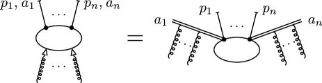
Figure 3: Graphical form of the decoupling relations for collinear and soft gluons. The relations show the decoupling of longitudinally polarized gluons, which are represented by curly lines. The $C^{+}$ ($C^{-}$) decoupling relation applies when the longitudinally polarized gluons all have momenta in the $C^{+}$ ($C^{-}$) singular region. The $S^{+}$ ($S^{-}$) decoupling relation applies when the longitudinally polarized gluons all have momenta in the $S$ singular region and the subdiagram that is represented by an oval contains only lines with momenta in the $C^{+}$ ($C^{-}$) singular region. The longitudinally polarized gluons are to be attached in all possible ways to the oval. The arrows on the gluon lines represent the factors $k^{\mu}\bar{n}^{\nu}/(k\cdot\bar{n})$ [$k^{\mu}n^{\nu}/(k\cdot n)$] that appear in the collinear (soft) approximation. The external lines with hash marks are truncated. In addition, the subdiagram can include any number of untruncated on-shell external legs (not shown), provided that the polarizations of the on-shell gluons are orthogonal to their momenta. $p_{i}$ are momenta, and the $a_{i}$ are color indices. The double lines are $C^{+}$, $C^{-}$, $S^{+}$, or $S^{-}$ eikonal lines, which are described in the text.

If any number of longitudinally polarized gluons carrying momenta in the $C^{+}$ ($C^{-}$) singular region attach in all possible ways to a subdiagram, then the $C^{+}$ ($C^{-}$) decoupling relation applies. The subdiagram can have any number of truncated external legs and any number of untruncated on-shell external legs, provided that the polarization of each on-shell gluon is orthogonal to its momentum. In the $C^{+}$ ($C^{-}$) case, the eikonal (double) lines shown in Fig. 3 have the Feynman rules that a vertex is $\mp igT_{a}\bar{n}_{1\mu}$ ($\pm igT_{a}\bar{n}_{2\mu}$) and a propagator is $i/(k\cdot\bar{n}_{1}-i\varepsilon)$ [$i/(k\cdot\bar{n}_{2}+i\varepsilon)$], where the upper (lower) sign in the vertex is for eikonal lines that attach to quark (antiquark) lines. Here, $T_{a}$ is an $SU(3)$ color matrix in the fundamental representation. (Our convention is that a QCD gluon-quark vertex is $igT_{a}\gamma_{\mu}$.) We call these eikonal lines $C^{+}$ and $C^{-}$ eikonal lines, respectively.

An analogous decoupling relation holds when any number of longitudinally polarized gluons with momenta in the soft singular region attach in all possible ways to a subdiagram that contains only lines with momenta in the $C^{+}$ ($C^{-}$) singular regions. Again, the subdiagram can have any number of truncated external legs and any number of untruncated on-shell external legs, provided that the polarization of each untruncated on-shell gluon is orthogonal to its momentum. In this case, the eikonal lines have the Feynman rules that a vertex is $\pm igT_{a}n_{1\mu}$ ($\mp igT_{a}n_{2\mu}$) and a propagator is $i/(k\cdot n_{1}+i\varepsilon)$ [($i/(k\cdot n_{2}-i\varepsilon)$] when the subdiagram is $C^{+}$ ($C^{-}$). We call these eikonal lines $S^{+}$ and $S^{-}$ eikonal lines, respectively.

The Feynman rules for the eikonal lines in the collinear and soft decoupling relations are summarized in Table 2.

Type	Vertex	Propagator
$C^{+}$	$\mp igT_{a}\bar{n}_{1\mu}$	$\displaystyle\frac{i}{k\cdot\bar{n}_{1}-i\varepsilon}$
$C^{-}$	$\pm igT_{a}\bar{n}_{2\mu}$	$\displaystyle\frac{i}{k\cdot\bar{n}_{2}+i\varepsilon}$
$S^{+}$	$\pm igT_{a}n_{1\mu}$	$\displaystyle\frac{i}{k\cdot{n}_{1}+i\varepsilon}$
$S^{-}$	$\mp igT_{a}n_{2\mu}$	$\displaystyle\frac{i}{k\cdot{n}_{2}-i\varepsilon}$

Table 2: Feynman rules for the collinear ($C^{\pm}$) and soft ($S^{\pm}$) eikonal lines. The upper (lower) sign is for the eikonal line that attaches to a quark (antiquark) line.

VI Factorization

Now let us describe the factorization of the contributions from the $C^{+}$, $C^{-}$, and $S$ singular regions.

We can determine the momentum assignments that give singular contributions by making use of the power-counting rules that we have outlined in Sec. III. When we apply these rules to the attachments of gluons with momenta in the singular regions, the symbol $\sim$ and the phrase “of the same order” mean that quantities do not differ by an infinite factor, while the phrases “much less than” and “much greater than” mean that quantities do differ by an infinite factor. Hence, for gluons with momenta in the singular regions, our convention that an allowed attachment of a gluon cannot change the essential nature of the momentum of the line to which it attaches has the following meaning: The attaching gluon cannot have an energy that is greater by an infinite factor than the energy of the line to which it attaches.

The rules in Sec. III lead to complicated relationships between the allowed momenta of gluons in a given diagrammatic topology. However, there is a general principle, which we have already mentioned, that allows us to organize the discussion: The attachments of gluons to a given line must be ordered so that a given attachment produces a virtuality along the line that is of order or greater than the virtualities that are produced by the attachments that lie to the outside of it. In particular, the virtuality that a $C^{\pm}$, $\tilde{C}^{\pm}$, or $S$ singular gluon produces on a $C^{\mp}$, $\tilde{C}^{\mp}$, or $S$ line is of order its energy times the energy of the line to which it attaches.

VI.1 Characterization of the singular contributions

The relationships between allowed momenta lead to a hierarchy of scales as the singular limits are approached. Consider, for example, the contribution in which an additional soft gluon is attached to the diagram of Fig. 2 to the same outgoing fermion lines as the other gluons, but to the outside of them. In order for this contribution to be leading, the additional soft gluon must produce a virtuality on the outgoing fermion lines that is of order or less than the virtuality of $D_{1}$ or $D_{3}$. The former condition implies that the energy scale of the additional soft gluon $\epsilon_{S}^{\prime}$ must be of order or less than $\epsilon^{+}(\eta^{+})^{2}$. Since $\epsilon_{S}\sim\epsilon^{+}$, this implies that $\epsilon_{S}^{\prime}\sim\epsilon_{S}(\eta^{+})^{2}$. That is, in the collinear singular limit, $\epsilon_{S}^{\prime}$ is infinitesimal with respect to $\epsilon_{S}$.

From such arguments it is clear that an infinite hierarchy of virtualities of various infinitesimal orders appears. However, these orders of virtuality are well separated in the singular limits. That is, the various gluon energy scales differ by infinite factors, as in our example. This property allows us to organize the singular contributions in such a way that we can apply the soft and $C^{\pm}$ approximations to obtain the factorized form.

In order to carry out the factorization, we need to distinguish two cases for the ordering of the energy scale of a collinear momentum relative to the energy scale of a soft momentum. Both of these orderings can yield contributions that are nonvanishing in the limits $\epsilon_{S}\to 0$, $\eta^{\pm}\to 0$.

Case 1: As $\epsilon_{S}\to 0$, $\epsilon^{\pm}/\epsilon_{S}$ is finite. (It is easy to see that the contribution in which $\epsilon^{\pm}/\epsilon_{S}$ goes to zero vanishes. See for example, Sec. IV.2.) In this case, we say that the collinear singular momentum and the soft singular momentum have energies that are of the same order.

Case 2: As $\epsilon_{S}\to 0$, $\epsilon_{S}/\epsilon^{\pm}\to 0$. In this case we say that the soft singular momentum has energy that is infinitesimal in comparison with the energy of the collinear singular momentum.

We will use an iterative procedure to factor gluons at the different levels of the hierarchy of energy scales. It is useful to establish first a general nomenclature to characterize this hierarchy of energy scales. We characterize each level in the hierarchy by the energy scale of the soft singular gluons in that level. We call that energy scale the “nominal scale”. We call soft singular and collinear singular gluons that have energies of order this scale nominal-scale gluons. We call collinear singular gluons that have energies that are infinitely larger than the nominal energy scale but infinitely smaller than the next-larger soft-gluon scale “large-scale” collinear gluons. The nominal-scale collinear gluons are of the type in case 1 above with respect to the nominal-scale soft gluons. The large-scale collinear gluons are of the type in case 2 above with respect to the nominal-scale soft gluons.

VI.2 Factorization of the singular contributions

Let us now describe the factorization of the singular contributions. We make use of an iterative procedure in which gluons of higher energies are factored before gluons of lower energies. As we shall see, this ordering of the factorization procedure is convenient because it allows us to apply the decoupling relations rather straightforwardly to decouple gluons whose attachments lie toward the inside of the Feynman diagrams before we decouple gluons whose attachments lie to the outside of the Feynman diagrams.

We will illustrate the factorization of the large-scale collinear gluons and the nominal-scale soft and collinear gluons for double light-meson production in $e^{+}e^{-}$ annihilation by referring to the diagram that is shown in Fig. 4. In this diagram, we have suppressed gluons with energies that are much less than the nominal scale. These gluons have attachments that lie to the outside of the attachments of the gluons that are shown explicitly. In the diagram in Fig. 4, each gluon represents any finite number of gluons, including zero gluons. For clarity, we have suppressed the antiquark lines in each meson and we have shown explicitly only the attachments of the gluons to the quark line in each meson and only a particular ordering of those attachments. However, we take the diagram in Fig. 4 to represent a sum of many diagrams, which includes all of the attachments that we specify in the arguments below of the singular gluons to the quark and antiquark in each meson, to other singular gluons, and to the $\tilde{H}$ subdiagram.

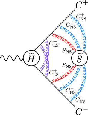
Figure 4: Diagram to illustrate the factorization of large-scale collinear gluons and nominal-scale soft and collinear gluons for double light-meson production in $e^{+}e^{-}$ annihilation. $C^{i}_{\textrm{LS}}$ denotes a large-scale $C^{i}$ singular gluon, $C^{i}_{\textrm{NS}}$ denotes a nominal-scale $C^{i}$ singular gluon, and $S_{\textrm{NS}}$ denotes a nominal-scale $S$ singular gluon.

VI.2.1 Factorization of the large-scale $C^{\pm}$ gluons

We begin with the large-scale $C^{\pm}$ gluons that have the largest energy scale, and proceed iteratively through all of the scales of the large-scale $C^{\pm}$ gluons. In the first step of the iteration, those are gluons with finite-energy collinear singular momenta. In the subsequent steps, only gluons with infinitesimal collinear singular momenta are present. Gluons with relatively infinitesimal energies may attach to a gluon that carries a $C^{\pm}$ singular momentum. We still consider that gluon to carry $C^{\pm}$ singular momentum.

First, we wish to apply the $C^{+}$ approximation and the $C^{+}$ decoupling relation (Fig. 3) to decouple the large-scale $C^{+}$ gluons that originate in the $\tilde{J}^{+}$ subdiagram from the $\tilde{H}$ and $\tilde{J}^{-}$ subdiagrams. In applying the decoupling relation, we need to know the extent of the subdiagram in Fig. 3: Eikonal lines appear at the points at which the subdiagram is truncated.

We include the attachments of gluons with large-scale $C^{+}$ momenta to the $\tilde{J}^{-}$ subdiagram that are allowed by our conventions and by power counting. Here, and in the discussions to follow, we consider a $C^{\pm}$ gluon to be attached to the $\tilde{J}^{\mp}$ subdiagram if and only if its momentum routes through $\tilde{H}$.

We include all of the attachments of gluons with large-scale $C^{+}$ momenta to $\tilde{H}$. We include the attachments that are allowed by our conventions and by power counting. However, we also include formally attachments to $\tilde{H}$ that yield vanishing contributions in the singular limits. (In subsequent iterations, we include formally, as well, the vanishing attachments of large-scale $C^{+}$ gluons to points on $C^{-}$ eikonal lines that lie to the interior of the outermost attachment of a $C^{-}$ singular gluon.)

In applying the $C^{+}$ decoupling relation, we do not include attachments of gluons with large-scale $C^{+}$ momentum to a gluon with nominal-scale $S$ momentum: Such attachments violate our convention for allowed attachments because they alter the nature of the $S$ singular momentum. However, as we mentioned above, gluons with nominal-scale $S$ singular momenta can attach to a gluon with large-scale $C^{+}$ singular momentum without altering the nature of the $C^{+}$ singular momentum. We carry these attachments along as we attach the gluon with finite $C^{+}$ singular momentum to other lines in the diagram. We follow this same procedure in discussions below in treating gluons whose energies are infinitesimal with respect to the energy of an $S$ or a $C^{\pm}$ singular gluon to which they attach.

The allowed attachments of gluons with large-scale $C^{+}$ momenta to a $C^{-}$ singular line lie to the inside of the attachments of gluons with nominal-scale $S$ or $C^{\pm}$ momenta. Therefore, one might expect that, when the $C^{+}$ decoupling relation is applied, a $C^{+}$ eikonal-line contribution would appear at the vertex immediately to the outside of the outermost allowed attachment of a large-scale $C^{+}$ gluon. In fact, such an eikonal-line contribution vanishes because the propagator on the $C^{-}$ singular line just to the outside of the outermost allowed attachment of a gluon with large-scale $C^{+}$ singular momentum is on shell, and, in the case of a gluon line, has physical polarization (polarization orthogonal to its momentum), up to relative corrections of infinitesimal size. Therefore, we omit such eikonal-line contributions in applying the decoupling relation.

Then, the result of applying the decoupling relation is that the gluons with large-scale $C^{+}$ momenta attach to $C^{+}$ eikonal lines that attach to the outgoing fermion lines in $\tilde{J}^{+}$ just to the outside of the $\tilde{H}$ subdiagram.

Next we decouple the gluons that originate in the $\tilde{J}^{-}$ subdiagram and have large-scale $C^{-}$ momenta from the $\tilde{H}$ and $J^{+}$ subdiagrams. The procedure follows the same argument as for the gluons with large-scale $C^{+}$ singular momenta, except for one new ingredient: We must include formally the vanishing attachments of the gluons with large-scale $C^{-}$ momenta to the $C^{+}$ eikonal lines from the previous step. Note that we need to include only the attachments that lie to the interior of the attachment of the outermost gluon with $C^{+}$ singular momentum in order to apply the $C^{-}$ decoupling relation. The result of applying the $C^{-}$ decoupling relation is that gluons with large-scale $C^{-}$ momenta attach to $C^{-}$ eikonal lines that attach to $C^{-}$ outgoing fermion lines just to the outside of the $\tilde{H}$ subdiagram.

Now, we iterate this procedure for the large-scale $C^{\pm}$ gluons at the next-lower energy scale. The result of applying the $C^{\pm}$ decoupling relations is that the large-scale $C^{\pm}$ gluons attach to $C^{\pm}$ eikonal lines that attach to the outgoing fermion lines just to the inside of the $C^{\pm}$ eikonal lines from the previous iteration. It is easy to see that, on each outgoing fermion line, the $C^{\pm}$ eikonal line from the current iteration can be combined with the $C^{\pm}$ eikonal line from the previous iteration into a single $C^{\pm}$ eikonal line. On the combined $C^{\pm}$ eikonal line, the attachments of $C^{\pm}$ gluons with the smaller energy scale lie to the outside of the attachments of gluons with the larger energy scale. (Other orderings yield vanishing contributions.) We continue iteratively in this fashion until we have factored all of the large-scale $C^{\pm}$ gluons. After this decoupling step, the sum of diagrams represented by Fig. 4 becomes a sum of diagrams represented by Fig. 5.

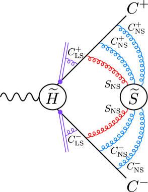
Figure 5: Diagram representing the sum of diagrams that occurs after one applies the decoupling of the large-scale collinear gluons that is described in Sec. VI.2.1.

VI.2.2 Factorization of the nominal-scale $C^{\pm}$ gluons

Next we factor the nominal-scale $C^{\pm}$ gluons. In applying the $C^{+}$ decoupling relation, we include the allowed attachments of these gluons to the $\tilde{J}^{-}$ subdiagram and the attachments to the nominal-scale soft gluons. We also include formally the vanishing contributions from the attachments of the nominal-scale gluons to the $\tilde{H}$ subdiagram and to the $C^{-}$ eikonal lines. Because of the ordering of virtualities along a line with $C^{+}$ singular momentum, the outermost attachment to such a line of a gluon with nominal-scale $C^{+}$ momentum must lie to the outside of the outermost attachment of a gluon with nominal-scale $S$ momentum. It is then easy to see that, for every attachment described above of a $C^{+}$ line to a line with momentum that is not $C^{+}$ singular, the $C^{+}$ approximation holds exactly. The $C^{-}$ propagator that lies to the outside of the outermost allowed attachment of a gluon with nominal-scale $C^{+}$ momentum to a line with $C^{-}$ singular momentum is on-shell, and, in the case of a gluon line, has physical polarization, up to relative corrections of infinitesimal size. Therefore, when we apply the $C^{+}$ decoupling relation, no eikonal line appears at the vertex immediately to the outside of this outermost attachment of a gluon with nominal-scale $C^{+}$ momenta. The result of applying the $C^{+}$ decoupling relation is that the nominal-scale $C^{+}$ gluons attach to several $C^{+}$ eikonal lines. These eikonal lines attach in the following locations: to the outgoing $C^{+}$ fermion lines just to the outside of $\tilde{H}$, but to the inside of the large-scale $C^{+}$ eikonal lines; just to the soft-gluon side of each vertex involving a nominal-scale soft gluon and a $C^{+}$ singular gluon of the large scale or a larger scale. In a similar fashion, we factor the nominal-scale $C^{-}$ gluons. The result of applying the $C^{-}$ decoupling relation is that the $C^{-}$ singular gluons attach to several $C^{-}$ eikonal lines. These eikonal lines attach to the following locations: to the outgoing $C^{-}$ fermion lines just to the outside of $\tilde{H}$, but to the inside of the large-scale $C^{-}$ eikonal lines; just to the soft-gluon side of each vertex involving a nominal-scale soft gluon and a $C^{-}$ singular gluon of the large scale or a larger scale. After this decoupling step, the sum of diagrams represented by Fig. 5 becomes the sum of diagrams represented by Fig. 6.

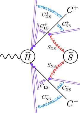
Figure 6: Diagram representing the sum of diagrams that occurs after one applies the initial decoupling of the nominal-scale collinear gluons that is described in Sec. VI.2.2.

VI.2.3 Factorization of the nominal-scale $S$ gluons

We now wish to apply the soft decoupling relations to factor the nominal-scale soft gluons. In order to do this, we implement the $S^{\pm}$ approximations for the attachments of the soft gluons to the $C^{\pm}$ singular lines of the large scale or a larger scale. However, we make a slight modification to the soft approximation by combining the momentum of the nominal-scale soft gluon with the total momentum of the associated nominal-scale $C^{\pm}$ eikonal line. Then, when we implement the $S^{\pm}$ decoupling relations, the nominal-scale $C^{\pm}$ eikonal lines are carried along with the nominal-scale soft-gluon attachments. In applying the $S^{+}$ decoupling relation, we include attachments of nominal-scale soft gluons to the $\tilde{J}^{+}$ subdiagram, and in applying the $S^{-}$ decoupling relation, we include attachments of nominal-scale soft gluons to the $\tilde{J}^{-}$ subdiagram. Because we have already factored the attachments of nominal-scale $C^{\pm}$ gluons, the $S^{\pm}$ approximations hold, up to relative corrections of infinitesimal size. We also include vanishing attachments of the nominal-scale soft gluons to the large-scale eikonal lines Collins:1985ue , including only those soft-gluon attachments that lie to the inside of the outermost $C^{+}$-gluon attachments. The $C^{\pm}$ propagator that lies to the outside of the outermost allowed attachment of a nominal-scale soft gluon to a $C^{\pm}$ line is on shell, up to relative corrections of infinitesimal size. Therefore, when we apply the $S^{\pm}$ decoupling relations, no $S^{\pm}$ eikonal lines appear at the vertices just to the outside of the outermost allowed attachments. The result of applying the $S^{\pm}$ decoupling relations is that soft gluons attach to $S^{\pm}$ eikonal lines. These eikonal lines attach to the outgoing $C^{\pm}$ fermion lines just to the outside of the nominal-scale $C^{\pm}$ eikonal lines and just to the inside of the large-scale $C^{\pm}$ eikonal lines. Associated with each attachment of a nominal-scale soft gluon to an $S^{\pm}$ eikonal line is a $C^{\pm}$ eikonal line to which nominal-scale $C^{\pm}$ gluons attach. After this decoupling step, the sum of diagrams represented by Fig. 6 becomes a sum of diagrams represented by Fig. 7.

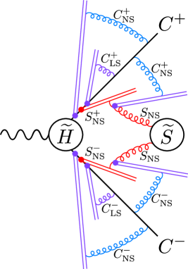
Figure 7: Diagram representing the sum of diagrams that occurs after one applies the decoupling of the nominal-scale soft gluons that is described in Sec. VI.2.3.

VI.2.4 Further factorization of the nominal-scale $C^{\pm}$ gluons

We next factor the nominal-scale $C^{\pm}$ gluons from the $S^{\pm}$ eikonal lines. In order do this, we include formally the vanishing contributions that arise when one attaches the nominal-scale $C^{\pm}$ gluons to all points on the $S^{\pm}$ eikonal lines that lie to the inside of the outermost attachment of a nominal-scale soft gluon. We also make use of the following facts: Each nominal-scale $C^{\pm}$ eikonal line that attaches to an outgoing $C^{\pm}$ fermion line is identical to the eikonal line that one would obtain by applying the $C^{\pm}$ decoupling relation to the attachments of the nominal-scale $C^{\pm}$ gluons to an on-shell fermion line; each nominal-scale $C^{\pm}$ eikonal line that attaches to a nominal-scale gluon is identical to the eikonal line that one would obtain by applying the $C^{\pm}$ decoupling relation to the attachments of nominal-scale $C^{\pm}$ gluon to an on-shell gluon line. Then, applying the $C^{+}$ decoupling relation, we find that the nominal-scale $C^{+}$ gluons attach to $C^{+}$ eikonal lines that attach to the outgoing fermion lines just to the inside of the large-scale $C^{+}$ eikonal lines. Similarly, applying the $C^{-}$ decoupling relation, we find that the nominal-scale $C^{-}$ gluons attach to $C^{-}$ eikonal lines that attach to the outgoing fermion lines just to the inside of the large-scale $C^{-}$ eikonal lines. This result is represented by the diagram that is shown in Fig. 8. The nominal-scale $C^{\pm}$ eikonal lines can then be combined with the large-scale $C^{\pm}$ eikonal lines. After performing those steps, we arrive at the final factorized form, which is represented by the diagram in Fig. 9.

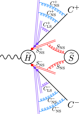
Figure 8: Diagram representing the sum of diagrams that occurs after one applies the further decoupling of the nominal-scale collinear gluons that is described in Sec. VI.2.4.

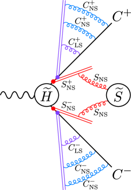
Figure 9: Diagram representing the sum of diagrams that occurs after one completely decouples the large-scale collinear gluons and the nominal-scale soft and collinear gluons.

VI.2.5 Completion of the factorization

Now we can iterate the procedure that we have given in Secs. VI.2.1–VI.2.4, taking the nominal scale to be the next-smaller soft-gluon scale. In these subsequent iterations, we include formally, in the steps of Secs. VI.2.1 and VI.2.2, the vanishing contributions from the attachments of the large-scale and nominal-scale $C^{+}$ and $C^{-}$ gluons to the soft gluons of higher levels and to the $S^{+}$ and $S^{-}$ eikonal lines that are associated with those soft gluons. (We also include formally the vanishing contributions from the attachments of the large-scale and nominal-scale $C^{+}$ and $C^{-}$ gluons to $\tilde{H}$, as in the first iteration.)

Proceeding iteratively through all of the soft-gluon scales, we produce new nominal-scale $S^{\pm}$ eikonal lines at each step that attach to the outgoing fermion lines just to the outside of the existing $S^{\pm}$ eikonal lines. The nominal-scale $C^{\pm}$ eikonal lines that attach to the outgoing $C^{\pm}$ fermion lines after the steps of Sec. VI.2.2 are situated just to the inside of these nominal-scale $S^{\pm}$ eikonal lines. After the further factorization of the nominal-scale $C^{\pm}$ gluons that is described in Sec. VI.2.4, the $S^{\pm}$ eikonal lines that attach to a given outgoing fermion can be combined into a single $S^{\pm}$ eikonal line. The soft gluons of a lower energy scale attach to the outside of the soft gluons of a higher energy scale. This is the only ordering that produces a nonvanishing contribution.

Following this procedure, we arrive at the standard factorized form for the singular contributions. The $\tilde{S}$ subdiagram now attaches only to $S^{+}$ eikonal lines that attach to the outgoing fermion lines from $\tilde{J}^{+}$ just outside of $\tilde{H}$ and to $S^{-}$ eikonal lines that attach to the outgoing fermion lines from $\tilde{J}^{-}$ just outside of $\tilde{H}$. The attachments involve only gluons with $S$ singular momenta. All of the $C^{\pm}$ singular contributions are contained in the $J^{\pm}$ subdiagram, which attaches via $C^{\pm}$ singular gluons to $C^{\pm}$ eikonal lines that attach to the outgoing fermion lines from $\tilde{J}^{\pm}$ just outside of the $S^{\pm}$ eikonal lines. This factorized form is illustrated in Fig. 10.

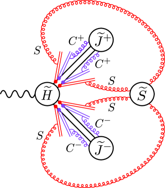
Figure 10: Illustration of the factorized form for double light-meson production in $e^{+}e^{-}$ annihilation. After the use of the decoupling relations, gluons with momenta in the $S$ singular region attach to $S^{\pm}$ eikonal lines and gluons with momenta in the $C^{\pm}$ singular regions attach to $C^{\pm}$ eikonal lines.

VI.3 Cancellation of the eikonal lines

At this point the $\tilde{S}$ subdiagram and associated soft eikonal lines, which we call $\bar{S}$, have the form of the vacuum-expectation value of a time-ordered product of four eikonal lines:

$$\bar{S}(x_{1q},x_{1\bar{q}},x_{2q},x_{2\bar{q}}) =$$

$$\langle 0|T\{[x_{1\bar{q}},\infty^{+}][\infty^{+},x_{1q}]\otimes[x_{2\bar{q}},\infty^{-}][\infty^{-},x_{2q}]\}|0\rangle_{S},$$

where

$$[x,y]=\exp\left[\int_{x}^{y}igT_{a}A_{\mu}^{a}dx^{\mu}\right]$$ (14)

is the exponentiated line integral (eikonal line) running between $x$ and $y$, $\infty^{+}=(\infty,0,\bm{0}_{\perp})$, and $\infty^{-}=(0,\infty,\bm{0}_{\perp})$. The symbol $\otimes$ indicates a direct product of the color factors that are associated with the soft-gluon attachments to meson 1 and the soft-gluon attachments to meson 2. We note that eikonal-line self-energy subdiagrams, which were absent in our derivation of $\bar{S}$, vanish for lightlike eikonal lines in the Feynman gauge. The subscript on the matrix element indicates that only contributions from the soft singular region are kept.

Because the $H$ and $J^{+}-\tilde{J}^{+}$ subdiagrams are insensitive to a momentum in the $S$ singular region flowing through them, we can ignore the difference between $x_{1q}$ and $x_{1\bar{q}}$ in Eq. (LABEL:S-tilde-me). Then the $S^{+}$ eikonal lines cancel. Note that this cancellation relies on the color-singlet nature of the external meson. In a similar fashion, we can ignore the difference between $x_{2q}$ and $x_{2\bar{q}}$ in Eq. (LABEL:S-tilde-me), and the $S^{-}$ quark and antiquark eikonal lines cancel.

We can make a Fierz rearrangement to decouple the color factors of the $\tilde{J}^{+}$ and $\tilde{J}^{-}$ subdiagrams from $\tilde{H}$. Then, we can write the $\tilde{J}^{\pm}$ subdiagrams and their associated eikonal lines, which we call $\bar{J}^{+}$ and $\bar{J}^{-}$, as follows:

$$\bar{J}^{\pm}_{\alpha\beta}(z_{i}) = \frac{P_{i}^{\pm}}{\pi}\int_{-\infty}^{+\infty}dx^{\mp}\exp[-i(2z_{i}-1)P_{i}^{\pm}x^{\mp}]\langle M_{i}(P_{i})|\bar{\Psi}_{\alpha}(x^{\mp})T\{[x^{\mp},\infty^{\mp}][\infty^{\mp},-x^{\mp}]\}\Psi_{\beta}(-x^{\mp})|0\rangle_{C^{\pm}}.$$ (15)

Here, $z_{i}$ is the fraction of $P_{i}^{\pm}$ that is carried by the quark in meson $i$, $\alpha$ and $\beta$ are Dirac indices, and the upper (lower) sign in Eq. (15) corresponds to $i=1$ ($i=2$). It is understood that the fields $\Psi$ and $\bar{\Psi}$ in the matrix element are in a color-singlet state. The subscripts on the matrix elements indicate that only the contributions from the collinear singular regions are kept.

There is a partial cancellation of the eikonal lines in $\bar{J}^{+}$ and $\bar{J}^{-}$, with the result that the residual eikonal lines run directly from $-x^{\mp}$ to $x^{\mp}$:

$$\bar{J}^{\pm}_{\alpha\beta}(z_{i})=\frac{P_{i}^{\pm}}{\pi}\int_{-\infty}^{+\infty}dx^{\mp}\exp[-i(2z_{i}-1)P_{i}^{\pm}x^{\mp}]\langle M_{i}(P_{i})|\bar{\Psi}_{\alpha}(x^{\mp})P[x^{\mp},-x^{\mp}]\Psi_{\beta}(-x^{\mp})|0\rangle_{C^{\pm}}.$$ (16)

Here, we have written the time-ordered product of the exponentiated line integral as a path-ordered product. Because the integrations over $z_{1}$ and $z_{2}$ have nonvanishing ranges of support in $\tilde{H}$, $x^{\mp}$ and $-x^{\mp}$ in Eq. (16) are typically separated by a distance of order $1/Q$. This shows that the $C^{\pm}$ singular contributions that have energies much less than $Q$ cancel, once they have been factored.

VI.4 Factorized form

We have shown that the contributions from $C^{\pm}$ singular regions factor from the $\tilde{J}^{\mp}$, $S$, and $H$ subdiagrams and are contained entirely in the $\bar{J}^{\pm}$ subdiagrams and that the contributions from the $S$ singular region factor from the $\tilde{J}^{\pm}$ subdiagrams and cancel. The $\bar{J}^{\pm}$ subdiagrams each have precisely the form of a meson distribution amplitude. Hence, we have arrived at the conventional factorized form, except for the following facts: the $\bar{J}^{\pm}$ subdiagrams contain only the infinitesimal $C^{\pm}$ singular regions, whereas they are conventionally defined to contain finite regions of integration; the $\tilde{H}$ subdiagram is not yet free of nonperturbative contributions from collinear momenta with transverse components of order $\Lambda_{\rm QCD}$ or less.

Next we extend the ranges of integration in the logarithmically ultraviolet divergent integrals in $\bar{J}^{\pm}$ from infinitesimal neighborhoods of the collinear singularities to finite neighborhoods that are defined by an ultraviolet cutoff $\mu_{F}\sim Q$, which is the factorization scale. In making such an extension, we do not encounter any new singularities in $\bar{J}^{\pm}$. The soft singularities that do not involve the eikonal lines have already been shown to cancel. There is the possibility that $S$ or $C^{\mp}$ singularities could arise from the eikonal lines in $\bar{J}^{\pm}$. However, as we have mentioned, after the cancellation of the quark and antiquark eikonal lines, the remaining segment of eikonal line is finite in length, with length of order $1/Q$. Hence, $S$ or $C^{\mp}$ modes with virtualities much less than $Q$ cannot propagate on these eikonal lines.

Finally, having extended the momentum ranges in $\bar{J}^{\pm}$, we redefine $\tilde{H}$ to be the factor that, when convolved with $\bar{J}^{\pm}$, produces the complete production amplitude. This is precisely the conventional definition of the hard subdiagram. Since the soft divergences have canceled and the collinear divergences are contained in $\bar{J}^{\pm}$, $\tilde{H}$ is a finite function (after ultraviolet renormalization), and depends only on the scales $Q$ and $\mu_{F}$ and the renormalization scale. Therefore, $\tilde{H}$ contains only contributions from momenta of order $Q$ or $\mu_{F}$, i.e., from momenta in the perturbative regime. We have now established the conventional factorized form for the production amplitude $\mathcal{A}$, which reads

$$\mathcal{A}=\bar{J}^{-}\otimes\tilde{H}\otimes\bar{J}^{+},$$ (17)

where the symbol $\otimes$ denotes a convolution over the longitudinal momentum fraction $z_{i}$ of the corresponding meson and we have suppressed the Dirac indices on $\bar{J}^{\pm}$ and $\tilde{H}$. The $\bar{J}^{\pm}$ are now given by Eq. (16), but without the subscript $C^{\pm}$ on the matrix element. They can be decomposed into a sum of products of Dirac-matrix and kinematic factors and the standard light-cone distributions for the mesons.

VI.5 Nonzero relative momentum between the quark and antiquark

Now let us return to the situation in which the $\bm{p}_{i\perp}$ in Eq. (1) are nonzero and of order $\Lambda_{\rm QCD}$. In this case the outgoing quark and antiquark in each meson are moving in slightly different light-cone directions. Therefore, we must define separate singular regions $C_{1q}$ ($C_{2q}$) for the quark direction and $C_{1\bar{q}}$ ($C_{2\bar{q}}$) for the antiquark direction in meson 1 (2).

As we have mentioned, in defining the collinear approximations, we can choose any auxiliary vectors $\bar{n}_{i}$ that, for the collinear singular region associated with $p_{i}$, satisfy the relation $\bar{n}_{i}\cdot p_{i}>0$. We choose the lightlike auxiliary vector $\bar{n}_{1}$, which is in the minus direction, for both the $C_{1q}$ and $C_{1\bar{q}}$ singular regions and the lightlike auxiliary vector $\bar{n}_{2}$, which is in the plus direction, for both the $C_{2q}$ and $C_{2\bar{q}}$ singular regions. That is, we take the same collinear approximation for the collinear regions associated with the quark and the antiquark in a meson. Then the factorization of the collinear singular regions goes through exactly as in the case $p_{\perp}=0$.

For gluons with momenta in the soft singular region, one can still define soft approximations, but the approximations are different for the couplings to lines in the quark and antiquark collinear singular regions. When gluons with momenta in the soft singular region attach to lines with momenta in the $C_{iq}$ ($C_{i\bar{q}}$) singular region, one can use a unit lightlike vector $n_{iq}$ ($n_{i\bar{q}}$) that is proportional to $p_{iq}$ ($p_{i\bar{q}}$) to define the soft approximation. Then, the gluons with momenta in the soft singular region still factor. However, in the factored form, the soft eikonal line that attaches to the quark (antiquark) line in meson $i$ is parametrized by the auxiliary vector $n_{iq}$ ($n_{i\bar{q}}$). Because $n_{iq}$ and $n_{i\bar{q}}$ differ by an amount of relative order $\lambda$ [Eq. (3)], the quark and antiquark soft eikonal lines in each meson fail to cancel completely. These noncancelling soft contributions violate factorization because they couple one meson to the other in the production amplitude.

If we take the approximation $n_{iq}=n_{i\bar{q}}$, but keep $n_{jq}\neq n_{j\bar{q}}$, then the quark and antiquark eikonal lines cancel in meson $i$, but not in meson $j$. However, the remaining soft subdiagram, which attaches only to the quark and antiquark eikonal lines in $\bar{J}$, can be absorbed into the definition of the $\bar{J}$ subdiagram for meson $j$. Therefore, we see that we obtain a violation of factorization only if the quark and antiquark eikonal lines fail to cancel in both mesons. Hence, the violations of factorization that arise from the soft function are of relative order $\lambda^{2}$.

In order to express the amplitude in terms of the light-cone distributions $\bar{J}^{\pm}$ in Eq. (15), it is necessary to neglect in $\tilde{H}$ the minus and transverse components of $p_{1q}$ and $p_{1\bar{q}}$ and the plus and transverse components of $p_{2q}$ and $p_{2\bar{q}}$. In doing so, we make an error of relative order $p_{i\perp}/Q\sim\lambda$.

VI.6 Failure of the soft cancellation for low-energy collinear gluons

Now let us discuss the cancellation of the soft diagram for the factorized form in which the soft subdiagram contains collinear gluons. As we have mentioned, such a factorized form is the one that would seem to follow most straightforwardly from SCET Bauer:2001yt ; Bauer:2002nz . Suppose that a gluon with momentum $k$ attaches to the soft eikonal line that attaches to the quark line in meson 1. That contribution contains a factor $1/k\cdot n_{1q}$, which is singular in the limit in which $k$ becomes collinear to $p_{1q}$ ($n_{1q}$). On the other hand, for the contribution in which the gluon with momenta $k$ attaches to the soft eikonal line that attaches to the antiquark line in meson 1, there is a factor $1/k\cdot n_{1\bar{q}}$, which is not singular in the limit in which $k$ becomes collinear to $p_{1q}$. Hence, the attachments of the gluon with momentum $k$ to the quark and antiquark lines fail to cancel when $k$ is in the $C_{1q}$ (or $C_{1\bar{q}}$) singular region. Furthermore, the uncanceled contribution is not suppressed by a power of $Q$ and is, in fact, divergent. Thus, we see that, in the factorized form in which the soft subdiagram contains collinear gluons, the soft subdiagram fails to cancel, and one cannot establish the conventional factorized form.. It might seem that one could recover the cancellation of the soft subdiagram by setting $p_{i\perp}$ exactly to zero. However, at $p_{\perp}=0$, the cancellation of the quark and antiquark eikonal lines becomes ill-defined for $k$ collinear to the quark and antiquark because of the infinite factors that arise from the eikonal denominators $k\cdot n_{1q}$ and $k\cdot n_{1\bar{q}}$. We note that this issue also arises in inclusive processes, for example the Drell-Yan process, in the decoupling of the soft subdiagram from color-singlet hadrons.

VII Summary

We have established, to all orders in perturbation theory, factorization of the amplitude for the exclusive production of two light mesons in $e^{+}e^{-}$ annihilation through a single virtual photon for the case in which the external mesons are represented by an on-shell quark and an on-shell antiquark. The case of on-shell external particles is important for perturbative matching calculations.

The presence of on-shell external particles opens the possibility of soft and collinear momentum modes of arbitrarily low energy. In this situation, low-energy collinear gluons can couple to soft gluons. That coupling leads to additional complications in the factorization proof. Nevertheless, we have shown that one can derive the standard factorized form, in which the production amplitude is written as a hard factor convolved with a distribution amplitude for each meson. The hard factor is free of soft and collinear divergences and depends only on the hard-scattering scale $Q$, the collinear factorization scale $\mu_{C}$, and an ultraviolet renormalization scale. The meson distribution amplitudes contain all of the collinear divergences and all of the nonperturbative contributions that involve virtualities of order $\Lambda_{\rm QCD}$ or less. We find that the factorization formula holds up to corrections of relative order $\Lambda_{\rm QCD}/Q$.

As an intermediate step in the factorization proof, we obtain a form in which the soft subdiagram does not contain gluons with momenta in the collinear singular regions. This form of factorization may be useful in the resummation of soft logarithms, as the contributions with two logarithms per loop are contained entirely in the jet functions, which are diagonal in color. It is essential in establishing the standard factorized form for exclusive processes with on-shell external partons because, as we have shown, the cancellation of the attachment of the soft diagram to a color-singlet hadron fails at leading order in $Q$ if the soft subdiagram would contain gluons with momenta that are collinear to the constituents of the hadron. This issue also arises in inclusive processes in the decoupling of the soft subdiagram from color-singlet hadrons.

In on-shell perturbative calculations in SCET, low-energy gluons with momenta collinear to the external particles can appear. At two-loop level and higher, these low-energy collinear gluons can couple to soft gluons. Since SCET has no provision to decouple the collinear gluons from the soft gluons, it seems that it would be most straightforward in SCET to treat the low-energy gluons as part of the soft contribution. In such an approach, the soft subdiagram contains gluons with momenta in both the soft and collinear singular regions. As we have said, the soft subdiagram would fail to cancel in this case, and one would not achieve the standard factorized form. Therefore, in the absence of a further factorization argument, there would be no assurance in a matching calculation that the low-virtuality contributions could all be absorbed into the meson distribution amplitudes: Some low-virtuality contributions might be associated with a soft function that could not be factored from the meson distribution amplitudes.

Alternatively, one could abandon the notion that SCET should reproduce the contributions of full QCD on a diagram-by-diagram basis and assume that SCET is valid only after one sums over all Feynman diagrams. Furthermore, one could consider the collinear action in SCET to apply to all collinear momenta of arbitrarily low energy. Then, as is asserted in Ref. Bauer:2002nz , the production amplitude in SCET would take the form of a hard-scattering diagram, a $\bar{J}^{+}$ light-cone distribution and a $\bar{J}^{-}$ light-cone distribution that are convolved with the hard subdiagram, and a soft subdiagram that is free of collinear momenta and that connects to the $\bar{J}^{+}$ and $\bar{J}^{-}$ light-cone distributions with interactions that are given by the collinear action. That factorized form is the one that we would obtain after the decoupling of the collinear gluons from the soft gluons if we were to extend the ranges of integration in the $\tilde{S}$, $\bar{J}^{+}$, and $\bar{J}^{-}$ subdiagrams from the singular regions to finite regions of $S$, $C^{+}$ and $C^{-}$ momenta. Issues of double counting arise when one extends the ranges of integration. They could be dealt with, for example, by making use of the method of zero-bin subtractions Manohar:2006nz . Once the double-counting issues are resolved, our proof shows that such a form for the amplitude is correct. However, this result does not follow obviously from QCD or from SCET. It requires a derivation, such as the one that we have given in this paper.

The low-energy contributions that we have discussed involve integrands that are homogeneous in the integration momenta. Therefore, one might argue that, if one applies the method of regions Beneke:1997zp , then such contributions lead to scaleless integrals and vanish. The difficulty in making use of such an argument to prove factorization is that the method of regions extends the range of integration for each region to infinity. There is no proof of the validity of such an extension, and, hence, there is the possibility of double counting. Double counting between the soft and collinear subdiagrams is dealt with in SCET through the use of zero-bin subtractions Manohar:2006nz . However, the zero-bin subtractions are formulated rigorously in terms of a hard cutoff. In Ref. Manohar:2006nz , examples of the zero-bin subtraction in dimensional regularization in one-loop perturbation theory are given. To our knowledge, no proof of an all-orders zero-bin subtraction scheme in dimensional regularization has been given.

In physical hadrons, gluon momenta are cut off by confinement at a scale of order $\Lambda_{\rm QCD}$. In that situation, one does not need to consider the possibility that collinear gluons can attach to soft gluons in order to demonstrate the factorization of nonperturbative contributions, i.e., those contributions that involve momentum components of order $\Lambda_{\rm QCD}$. However, if one wishes to factor logarithmic contributions up to a scale of order $Q$, for example, for the purpose of resummation, then it is again necessary to treat the attachments of collinear gluons to soft gluons along the lines that we have described in this paper.

In this paper, we have focused on a specific exclusive process. However, we expect that our method can be generalized straightforwardly to the other exclusive processes and, possibly, to inclusive processes. In the latter case, one must consider Glauber-type momenta explicitly, as contributions that arise from such momenta cancel only once one has summed over all possible final-state cuts Bodwin:1984hc ; Collins:1983ju ; Collins:1985ue ; Collins:1988ig ; Collins:1989gx . However, it seems plausible that one can implement this cancellation, using standard techniques, independently of the factorization arguments that we have presented here.

- (1) C. W. Bauer, S. Fleming, D. Pirjol, and I. W. Stewart, Phys. Rev. D 63, 114020 (2001) [arXiv:hep-ph/0011336].
- (2) C. W. Bauer, D. Pirjol, and I. W. Stewart, Phys. Rev. D 65, 054022 (2002). [arXiv:hep-ph/0109045]
- (3) C. W. Bauer et al., Phys. Rev. D 66, 014017 (2002). [arXiv:hep-ph/0202088]
- (4) G. T. Bodwin, X. Garcia i Tormo, and J. Lee, Phys. Rev. Lett. 101, 102002 (2008) [arXiv:0805.3876 [hep-ph]].
- (5) A. V. Manohar, Phys. Lett. B 633, 729 (2006) [arXiv:hep-ph/0512173].
- (6) A. V. Manohar and I. W. Stewart, Phys. Rev. D 76, 074002 (2007) [arXiv:hep-ph/0605001].
- (7) G. T. Bodwin, Phys. Rev. D 31, 2616 (1985) [Erratum-ibid. D 34, 3932 (1986)].
- (8) J. C. Collins, D. E. Soper, and G. Sterman, Nucl. Phys. B 261, 104 (1985).
- (9) J. C. Collins, D. E. Soper, and G. Sterman, Adv. Ser. Direct. High Energy Phys. 5, 1 (1988). [arXiv:hep-ph/0409313]
- (10) J. C. Collins, ANL-HEP-PR-84-36 (1984).
- (11) G. Sterman, Nucl. Phys. B 281, 310 (1987).
- (12) H. Contopanagos, E. Laenen, and G. Sterman, Nucl. Phys. B 484, 303 (1997) [arXiv:hep-ph/9604313].
- (13) N. Kidonakis, G. Oderda, and G. Sterman, Nucl. Phys. B 525, 299 (1998) [arXiv:hep-ph/9801268].
- (14) N. Kidonakis, G. Oderda, and G. Sterman, Nucl. Phys. B 531, 365 (1998) [arXiv:hep-ph/9803241].
- (15) G. Sterman and M. E. Tejeda-Yeomans, Phys. Lett. B 552, 48 (2003) [arXiv:hep-ph/0210130].
- (16) A. Sen, Phys. Rev. D 28, 860 (1983).
- (17) J. C. Collins, D. E. Soper, and G. Sterman, Nucl. Phys. B 223, 381 (1983).
- (18) G. Sterman, Phys. Rev. D 17, 2773 (1978).
- (19) S. B. Libby and G. Sterman, Phys. Rev. D 18, 4737 (1978).
- (20) G. T. Bodwin, S. J. Brodsky, and G. P. Lepage, Phys. Rev. Lett. 47, 1799 (1981).
- (21) C. W. Bauer, D. Pirjol, and I. W. Stewart, Phys. Rev. D 67, 071502 (2003). [arXiv:hep-ph/0211069].
- (22) M. Beneke, G. Buchalla, M. Neubert, and C. T. Sachrajda, Nucl. Phys. B 591, 313 (2000) [arXiv:hep-ph/0006124].
- (23) V. A. Smirnov, Phys. Lett. B 465, 226 (1999). [arXiv:hep-ph/9907471]
- (24) G. Sterman, Phys. Rev. D 17, 2789 (1978).
- (25) G. Grammer, Jr. and D. R. Yennie, Phys. Rev. D 8, 4332 (1973).
- (26) J. C. Collins and D. E. Soper, Nucl. Phys. B 193, 381 (1981) [Erratum-ibid. B 213, 545 (1983)].
- (27) M. Beneke and V. A. Smirnov, Nucl. Phys. B 522, 321 (1998) [arXiv:hep-ph/9711391].
- (28) J. C. Collins, D. E. Soper, and G. Sterman, Phys. Lett. B 134, 263 (1984).
- (29) J. C. Collins, D. E. Soper, and G. Sterman, Nucl. Phys. B 308, 833 (1988).