Time integration and steady-state continuation for 2d lubrication equations

Abstract

Lubrication equations describe many structuring processes of thin liquid films. We develop and apply a numerical framework suitable for their analysis employing a dynamical systems approach. In particular, we present a time integration algorithm based on exponential propagation and an algorithm for steady-state continuation. Both algorithms employ a Cayley transform to overcome numerical problems resulting from scale separation in space and time. An adaptive time-step allows one to study the dynamics close to hetero- or homoclinic connections. The developed framework is employed on the one hand to analyze different phases of the dewetting of a liquid film on a horizontal homogeneous substrate. On the other hand, we consider the depinning of drops pinned by a wettability defect. Time-stepping and path-following are used in both cases to analyze steady-state solutions and their bifurcations as well as dynamic processes on short and long time-scales. Both examples are treated for two- and three-dimensional physical settings and prove that the developed algorithms are reliable and efficient for 1d and 2d lubrication equations.

1 Introduction

The dynamics of structuring processes of thin liquid films, ridges and drops on solid substrates is often described by thin film or lubrication equations. They are obtained employing a long wave approximation [62]. The notion ’thin’ means that the thickness of the film/drop is small as compared to all typical length scales parallel to the substrate. Thin film equations model, for instance, dewetting due to van der Waals forces [72, 57, 78, 95, 3], the long-wave Marangoni instability of a film heated from below [63, 11, 90], and the evolution of a film of dielectric liquid in a capacitor [52, 100, 56, 43]. Including driving forces parallel to the substrate allows one to describe, e.g., droplets that slide down an incline under gravity under isothermal [66, 96] and non-isothermal conditions [11, 90], the evolution of transverse front instabilities [81, 6, 29, 44, 89], and the evolution of shocks in films driven by a surface tension gradient against gravity [9, 82]. Extensions describe, for instance, two-layer films, films with soluble or non-soluble surfactants, films of colloidal suspensions, and effects of evaporation, complex rheology or slip at the substrate. For reviews see, e.g. references [62, 45, 93, 12].

Thin film equations are related to other ’standard’ equations employed in studies of pattern formation out of equilibrium [22]. For instance, the (convective) Cahn-Hilliard and the Kuramoto-Sivashinsky equation may be obtained from a thin film equation for sliding drops and flowing films as limiting cases for small and large lateral driving, respectively [90].

Due to the strong non-linearity a typical thin film equation is difficult to handle numerically, in particular, when describing three-dimensional physical situations resulting in a partial differential equation (PDE) with two spatial dimensions (2d). We develop and apply a numerical framework to study the time evolution and to follow steady state solutions in parameter space for 1d and 2d equations. For viscous fluids (small Reynolds number flows), for a surface tension that dominates over viscosity (small capillary number), and a small lateral driving force the long wave approximation results in the following evolution equation for the film thickness or drop profile $h(x,y,t)$ [62, 45]

$$\partial_{t}h\,=\,-\nabla\cdot\left[m(h)\nabla\tilde{p}(h)+\vec{\mu}(h)\right],$$ (1)

where $m(h)$ is a mobility function, $\vec{\mu}(h)$ represents the lateral driving force, and the pressure $\tilde{p}(h)$ may contain several terms. A curvature or Laplace pressure results from capillary and stabilizes a flat film. Its contribution results in a Bilaplacian of the height $h$. That is the highest order derivative in the equation. Therefore it constitutes one of the main numerical difficulties. Pressure contributions that destabilize the flat film can result from various physical mechanisms [62]. Examples include an electrostatic pressure for dielectric liquids in a capacitor [52, 56, 100], a disjoining or conjoining pressure for very thin films below 100 nanometers thickness resulting from effective molecular interactions between the substrate and the free surface (wettability effects) [24, 26, 40], a ’thermal pressure’ for a thin film on a heated plate (when the long-wave Marangoni mode is dominant) [60, 11] and a hydrostatic pressure due to gravity, e.g., for a fluid film under a ceiling [30, 25, 14]. All the mentioned destabilizing effects result in a long-wave instability, i.e., an instability with wavenumber zero at onset. Here we use two variants of a disjoining pressure as examples for a destabilizing mechanism because their particular thickness dependencies are numerically demanding and extensive literature results allow for detailed comparison. However, the developed algorithms can be readily applied to any other combination of stabilizing and destabilizing pressure terms.

In the absence of a lateral driving force ($\mu=0$), a film that is linearly unstable evolves during a short-time evolution into a structure of holes, drops or mazes with a typical structure length determined by film thickness and other control parameters that reflect the character of the destabilizing phenomenon [70, 78, 60, 48, 10, 11, 75]. This process is often called ’spinodal dewetting’ [57]. However, the resulting short-time structure is unstable (representing a saddle in function space) with respect to coarsening and on a large time-scale the structures coarsen until the system eventually approaches the global energetic minimum, i.e., a single drop or hole [7, 33, 86]. Indeed without a lateral driving force the system follows a relaxation dynamics and the evolution equation can be written using the variation of an underlying energy functional [63, 57, 85]. The variational form of the (then coupled) evolution equations can also be derived for multilayer films in similar settings [67, 68]. However, even in the one-layer case, details of the different phases of the process are still under investigation. Examples include the initial structuring process that might occur via nucleation or a surface instability [95, 3], and the mechanisms of the transverse instability of dewetting fronts [79, 71].

A detailed understanding of dewetting films and the other processes listed above is only possible if the pathways of time-evolution and the steady states described by Eq. (1) can be determined in the one- and two-dimensional case using fast and versatile algorithms. As the steady drop solutions in 1d can be seen as periodic trajectories in a conservative dynamical system one can use available continuation packages for ordinary differential equations [28] to map different solution families and their linear stability (see, e.g., [97, 90, 94]). Careful interpretation allows one, e.g., to predict for dewetting films the dominance of different rupture mechanisms within the linear unstable parameter range [95, 97, 83]. No such continuation tools are, however, available in the two-dimensional case.

The situation is more involved when lateral driving forces are present, i.e., gravity on an incline [66], or temperature gradients along the substrate [17, 46, 8]. There, new phenomena appear like transverse instabilities of sliding liquid ridges, advancing and receding fronts [81, 6, 29, 96, 89]. Another fascinating finding is related to sliding drops: Beyond a critical driving force the drop forms a cusp at the back end and ’emits’ smaller satellite drops [66, 5, 50]. For a driven contact line, heterogeneities of the substrate can cause a stick-slip motion [24]. In the setting of a sliding drop this leads at a critical driving force to the depinning of drops from such localized heterogeneities. In the vicinity of the responsible sniper bifurcation the resulting motion resembles stick-slip motion: The drop sticks a long time at a wettability defect and then suddenly slips to the next defect. This was studied in the 1d case in Refs. [92, 91]. Differences in time scales for the stick- and the slip-phase may be many orders of magnitude. On the homogeneous substrate one can, in the 1d case, regard stationary periodic drop and surface wave solutions as periodic trajectories of a dissipative dynamical system. They emerge from the trivial flat film state via a Hopf bifurcation [90]. This allows one to employ standard continuation packages [28] to obtain solution families and to track the various occurring bifurcations [96, 42, 94, 87]. The same applies for fronts (shocks) and drops that correspond to heteroclinic and homoclinic orbits, respectively [9, 58, 20]. Note, however, that at present little is known about the solution and bifurcation structure in the 2d case.

In the previous decade many publications were devoted to the numerical study of thin film dynamics. Studies focus, e.g., on drop spreading for wetting liquids [103, 36, 27, 102], heated films [60, 36, 11] pending drops [36, 35], and the dewetting of partially wetting films [78, 61, 10, 102]. The analysis of different numerical approaches [103, 36, 27, 102, 35] leads to the conclusion that the positivity ($h\geq 0$) and the convergence of discrete solutions as well as the performance of the algorithm depend on the way the mobility $m(h)$ is discretized. However, here, the preservation of positivity is less of a problem because there exists the precursor film. Moreover, such a positivity preserving scheme [103] applied to our partial wetting model may lead to stability problems (spatial oscillations) when the drop height is much larger than the precursor film. Indeed, as pointed out by Grün [35] the stability results only apply if the disjoining pressure $\Pi(h)$ remains bounded from below (when $h\rightarrow 0$). Most of the disjoining pressures employed in the literature are unbounded as the ones that we will use. Therefore, here the preservation of positivity is not a crucial stability criteria. The classical way to overcome stability problems is to employ a semi-implicit scheme (see, e.g., [11]). The implicit part corresponds to the bilaplacian, i.e. the linear operator of highest order which should be related to the eigenvalues of large modulus [99]. The approach normally works well if the ratio of drop height and precursor film thickness is small. However, for larger drops simulations often display spatial numerical oscillations.

We conclude that reliable algorithms for time integration and path-following for steady state solutions that are applicable equally well in most of the above introduced examples are not readily available. Here, we develop and apply a time integration scheme with an adaptive time-step and tools for bifurcation analysis that are applicable in the 1d and (most importantly) 2d case.

Our starting point is the understanding that not only mobility is crucial for the numerical stability but also the disjoining pressure. Thus, in a semi-implicit scheme, a good choice of the linear part should contain contributions from these terms (see below section 2.4). A natural candidate is the Jacobian matrix at each time-step. Another efficient time integrator which involves the Jacobian matrix is the exponential propagation scheme. In general, it is more stable and converges better than semi-implicit methods [98]. The exponential propagation scheme is based on the exact solution of the linearized equation at each time-step requiring the computation of the exponential of the Jacobian matrix. This operator is not directly computed: As commonly practiced for large and sparse matrices, only its action on vectors is estimated using projections on small Krylov subspaces of dimension $K\ll N$ [73]. The standard algorithm to perform this task is the Arnoldi procedure possibly incorporating improvements as proposed in [98]. The exponentiation can be performed at a negligible cost as long as $K$ is not too large.

The application of such a scheme to lubrication equations proves to be reliable. However, the approximation in Krylov subspaces converges rather slowly. We show that the necessary dimension $K$ is about one hundred while in Refs. [31, 73, 38, 98] $K\approx 10$ is sufficient. The difference results from the presence of the fourth order Bilaplacian in lubrication equations. Its effect is more disadvantageous than the one of a second order operator because the magnitude of the large negative eigenvalues increases with the order of the differentiation operator [51]. To our knowledge, no literature study analyzes the efficiency of the Krylov subspace approximation to a matrix exponential operator that contains a fourth order operator. We improve this step by coupling existing methods for the determination of the rightmost spectrum with the classical Arnoldi procedure [55]. In particular, the application of a Cayley transform proves to be most powerful. The resulting scheme is well suited to efficiently adapt the time-step to the corresponding time-scale of the dynamics. This allows for very large time-steps as, for instance, in problems involving coarsening and stick-slip drop motion.

The outlined scheme can not only be used for time-stepping. We show that the Krylov reduction associated with the Cayley transform can as well be applied to track steady states in parameter space employing a continuation scheme that consists of the determination of a tangent predictor, the application of Newton’s algorithm along the secant direction, the detection of bifurcation points and finally the determination of the direction of bifurcating branches of steady solutions [76]. Note, that in both algorithms, time-stepping and continuation, the Cayley transform is used in a original and to our knowledge novel way.

The paper is structured as follows. Section 2 presents the lubrication equation and its spatial discretization. Then we describe in Section 3 the exponential propagation method and discuss different ways to exponentiate the Jacobian. In Section 4 we adapt the developed algorithms to employ them for the continuation of steady states. Two appendices give details for the Krylov reductions (A) and convergence of the algorithms (B). In the remaining part, we apply the algorithms to two typical situations. The first one (Section 5) is the dewetting process of a thin film on a horizontal substrate. The slow coarsening process that follows the initial fast patterning provides an excellent test for the adaption of the time-step. We do as well study steady state solutions in 2d, in particular, we discuss several solution branches corresponding to quadratic and hexagonal arrays of drops. Second, in Section 6 we study the pinning/depinning of drops on an inclined heterogeneous substrate. The path-following algorithm is applied to determine branches of steady state solutions and, in consequence, the onset of depinning in the 2d case. The stick-slip motion of drops beyond depinning is investigated using our time-stepping algorithm. For comparison with the literature we do as well provide selected results for the 1d case. Our conclusions are found in Section 7.

2 Modeling and Spatial Discretization

2.1 Lubrication equation

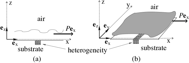
Fig. 1: Sketch of the (a) two-dimensional and (b) three-dimensional physical setting of the problem: A free-surface liquid film rests or flows on a possibly heterogeneous substrate. Thereby the heterogeneous wettability is assumed to depend on the location in the $x$-direction only. A driving force $P$ might act along the $x$-direction. Note, that the resulting film evolution equations have one (a) and two (b) spatial dimensions and are referred to as the 1d and 2d case, respectively.

Consider a liquid layer on an (inhomogeneous) one- or two-dimensional solid substrate (Fig. 1). The liquid partially wets the substrate and might be subject to a constant lateral force $P$. Using the long-wave approximation, the dimensionless evolution equation for the film thickness profile $h(x,y,t)$ derived from the Navier-Stokes equations, continuity and boundary conditions is [62, 45]

$$\partial_{t}h=F(h,x)=-\nabla\cdot\left\{m(h)\left[\nabla\left(\Delta h+\Pi(h,x)\right)+P\mathbf{e_{x}}\right]\right\}$$ (2)

where $\nabla=(\partial_{x},\partial_{y})$ is the planar gradient operator and $\Delta=\partial_{xx}^{2}+\partial_{yy}^{2}$ is the planar Laplacian. Note, that Eq. (2) has one and two spatial dimensions for two- and three-dimensional physical settings, respectively. In the following they are referred to as the 1d and 2d case, respectively. The mobility function $m(h)=h^{3}$ corresponds to Poiseuille flow without slip at the substrate. The term $\Delta h$ represents the Laplace pressure. Wettability is modeled by the disjoining pressure $\Pi(h,x)$ that for a striped heterogeneous substrate depends on film thickness and on the position $x$. Here, the lateral force acts as well in the $x$-direction (Fig. 1). Many particular forms of the disjoining pressure are discussed [24, 45, 12]. The most common ones allow for the presence of an ultra-thin wetting layer (a so-called ’precursor film’) of about 1-10 nm thickness. The short-time dewetting dynamics of an unstable film results in large amplitude structures, either drops or holes. It is often called initial ’film rupture’ even if a stable precursor film remains present – a convention we follow.

To facilitate comparison to the literature we employ the disjoining pressures

$$\Pi(h)=-2e^{-h}(1-e^{-h})-Gh$$ (3)

(as used in [96, 97]), and

$$\Pi(h)=-\frac{b}{h^{3}}+e^{-h}$$ (4)

(as used in [77, 95]). We call them (I) and (II), respectively. For case (II) we incorporate varying wettability properties due to a heterogeneous coating as

$$\Pi(h,x)=\frac{b}{h^{3}}-\left[1+\epsilon\xi(x)\right]e^{-h},$$ (5)

where $\xi(x)$ is the heterogeneity profile and $\epsilon$ the amplitude of the heterogeneity (as in [92, 91]).

2.2 Functional space

The considered domain is $D=[0;L]$ (1d case) or $D=[0;L_{x}]\times[0;L_{y}]$ (2d case). Eq. (2) defines a partial differential equation (PDE) in $H^{4}(D)$

$$\partial_{t}h=F(h,x),h\in H^{4}(D)$$ (6)

To obtain a well posed PDE system, we introduce periodic boundary conditions. In the studied case of non-volatile liquids the mass $M=\int_{D}h(x,y)dxdy$ is conserved. If $S_{D}$ denotes the surface of the domain $D$, the measure $H=M/S_{D}$ represents the mean height and $u=h-H$ is the perturbation (sometimes denoted $\delta h$). The PDE (6) defined in the space

$$E_{0}= \left\{u\in H^{4}(D):\int_{D}u(x,y)dxdy=0\right.$$ (7)

$$\left.\mbox{and periodicity of}\quad\partial_{x}^{i}u\quad\mbox{and}\quad\partial_{y}^{j}u,\mbox{}0\leq i,j\leq 3\right\}$$

is well defined: (i) $F$ operates on the Euclidian space $\{H+E_{0}\}$, and (ii) linear operators operate on the linear space $E_{0}$. In this space, we define the $L^{2}$ norm (denoted $||.||$) of $u$:

$$||u||=||\delta h|| = \frac{1}{S_{D}}\left(\int_{D}|u(x,y)|^{2}dxdy\right)^{1/2},$$ (8)

where $|u|$ is the Euclidean. The notation $||\delta h||$ is used for the presentation of the numerical results while $||u||$ is reserved for the description of the algorithm.

2.3 Spatial discretization

Here, we devote much effort to the time integration but chose the spatial discretization as simple and generic as possible. A finite difference scheme is used associated with a regular meshing of the domain. We use in $x$ and $y$ directions, $(N_{x}+1)$ and $(N_{y}+1)$ mesh points at distances $\delta x=N_{x}/L_{x}$ and $\delta y=N_{y}/L_{y}$, respectively. The number of discretization points is $N=(N_{x}+1)\times(N_{y}+1)$ in the 2d case and $N=N_{x}+1$ in the 1d case. The differentiation operators are approximated by a centered five-point stencil, i.e., for the Bilaplacian $\Delta^{2}$ and the third order operator $\nabla\Delta$ it is a second-order approximation while for the gradient or divergence operator $\nabla$ and the Laplacian $\Delta$ it is a fourth-order approximation. Thus, these operators are sparse band matrices with maximally 5 (1d) or 25 (2d) non-zero elements in each row. The map $F(h,x)$ defined in Eq. (6) is discretized according to Eq. (2), i.e., in the mass conserving form. The Jacobian of the map $F$ is discretized using Eq. (2.4) below, resulting in a second-order approximation. The discretized Jacobian matrix is not in a mass conserving form to avoid a further increase of the number of non-zero elements. Mass conservation is, however, imposed during the Krylov projection (see appendix A).

2.4 Jacobian matrix

Next, we justify our choice to compute the Jacobian matrix at each time-step. First, we explicitly determine the Jacobian matrix as linearization of the function $F(h,x)$ at $h=h_{0}$

$$\mathbf{J}=D_{h}F(h_{0},x)$$ (9)

where $D_{h}$ denotes the differentiation operator with respect to $h$. The Jacobian matrix is a sum of differentiation operators up to fourth order:

$$\mathbf{J}u = v_{0}(h_{0},x)u+{\mathbf{v_{1}}}(h_{0},x)\cdot\nabla u$$

$$+m_{0}\Pi^{\prime}_{0}\Delta u-\nabla m_{0}\cdot\nabla\Delta u-m_{0}\Delta^{2}u.$$

with

$$v_{0}(h_{0},x) = -m^{\prime}_{0}\Delta^{2}h_{0}-P\partial_{x}m^{\prime}_{0}$$

$$+m^{\prime}_{0}\Delta\Pi_{0}+\nabla m^{\prime}_{0}\cdot\nabla\Pi_{0}+\nabla m\cdot\nabla\Pi^{\prime}_{0}+m\Delta\Pi^{\prime}_{0}$$

$$\mathbf{v_{1}}(h_{0},x) = -m^{\prime}_{0}\nabla\Delta h_{0}+m^{\prime}_{0}\nabla\Pi_{0}+2m_{0}\nabla\Pi^{\prime}+\nabla m_{0}\Pi^{\prime}+P\mathbf{e_{x}}$$ (12)

and

$$\begin{array}[]{lcrclcr}m_{0}&=&m(h_{0})&&m^{\prime}_{0}&=&\frac{dm}{dh}(h_{0})\\ \Pi_{0}&=&\Pi(h_{0},x)&&\Pi^{\prime}_{0}&=&\frac{d\Pi}{dh}(h_{0},x)\end{array}$$

The Jacobian matrix $\mathbf{J}$ has eigenvalues with large negative real parts. They correspond to the fastest time scales related to the differentiation operators. As these eigenvalues are situated in the left half of the complex plane they are called “leftmost eigenvalues”. Their presence is the main cause for spatial numerical oscillations in explicit time integration methods. The resulting stability restriction on the time-step is overcome by treating the linear term implicitly. The leftmost eigenvalues are due to the differentiation operator of the highest degree. Therefore, on can filter them out by treating only this operator implicitly. The implicit linear term normally corresponds to the Laplacian for second order equations like, e.g., reaction-diffusion or Navier-Stokes equations and to the bilaplacian for fourth order equations like, e.g., the Kuramoto-Sivashinsky equation [32]. Here, a natural candidate is the bilaplacian. However, it is multiplied by the Poiseuille flow mobility $m_{0}=h_{0}^{3}$. This implies that, e.g., for a height variation by a factor 10 like for a drop solution, a factor $10^{3}$ appears in the linear operator. The resulting spatial scale separation complicates the situation as compared, e.g., to the Kuramoto-Sivashinsky equation.

Furthermore, here the lower order operators may contribute to the leftmost eigenvalues because the vectorial factor in front of them can have very large elements. For example, the Laplacian is scaled by $m_{0}\Pi^{\prime}_{0}$ related to the disjoining pressure that can be very large close to the contact region of drops. Then the Laplacian gives a non-negligible contribution to the leftmost spectrum of $\mathbf{J}$. This strongly localized prefactor is reminiscent of a point force at the contact line related to wettability as discussed, e.g., in [24]. Thus the specific numerical problems of the thin film equation for partially wetting liquids are not only due to the Poiseuille flow mobility but also to phenomena related to wettability and contact angle.

In conclusion, it is not advisable to filter the leftmost eigenvalues employing a constant linear operator since flow maxima and front positions are time dependent. It is preferable to compute the Jacobian through a linearization at each time-step. It is then employed in the exponential propagation method as it is best suited to our purpose (cf. introduction and appendix B).

3 Time integration

3.1 Exponential propagation

Starting from the known profile $h_{0}$ at $t_{0}$, the exponential propagation scheme consists in solving the autonomous evolution problem

$$\frac{dh}{dt} = F(h,x),$$ (13)

$$h(t_{0}) = h_{0}$$ (14)

at each time-step. This is done by expanding the operator $F(h,x)$ near the state $h_{0}$ in a Taylor series

$$F(h_{0}+u,x)=F(h_{0},x)+D_{h}F(h_{0},x)u+R(u),$$ (15)

where $D_{h}F(h_{0},x)$ is the Jacobian matrix at $h_{0}$ and $R(u)=O(||u||^{2})$ contains the quadratic and higher order terms. To simplify the notation we let

$$\mathbf{J} = D_{h}F(h_{0},x)$$ (16)

$$b = F(h_{0},x).$$ (17)

The height variation $u(\tau)=h(t_{0}+\tau)-h_{0}$ then solves the evolution problem

$$\frac{du}{d\tau} = b+\mathbf{J}u+R(u),$$ (18)

$$u(0) = 0$$

which admits as solution

$$u(\tau)=G(\mathbf{J}\tau)b\tau+\int_{0}^{\tau}\exp((\tau-\tau^{\prime})\mathbf{J})R(u(\tau^{\prime}))d\tau^{\prime},$$ (19)

with

$$G(\mathbf{J}\tau)=\frac{\exp(\mathbf{J}\tau)-\mathbf{I}}{\mathbf{J}\tau}.$$ (20)

Eq. (20) is formally correct even if $\mathbf{J}$ is not invertible since the operator $G$ can be expressed as the series $G(x)=\sum_{n=0}^{+\infty}x^{n}/(n+1)!$. Since the functions $G$ and $\exp$ tend to zero at $-\infty$, they filter the leftmost spectrum of the operator $\mathbf{J}$. For a semi-implicit scheme one has a similar situation: There is a rational function of $\mathbf{J}$ that plays the role of the filter. Yet, a rational function tends slower to zero than $G$ and $\exp$ when approaching $-\infty$. Therefore, we expect the exponential propagation scheme to better filter the leftmost eigenvalues. See as well appendix B.

3.2 Order of the scheme and error estimator

If we only consider linear variations of $F(h,x)$, i.e., $R(u)\equiv 0$ in Eq. (15), the first term of Eq. (19) is the exact solution of the evolution problem (18):

$$u^{(1)}(\tau)=G(\mathbf{J}\tau)b\tau.$$ (21)

The solution $h^{(1)}(\tau)=u^{(1)}(\tau)+h_{0}$ is then an approximation of second order with respect to time. To employ exponential schemes of higher order one has to take into account the non-linear term $R(u)$ in Eq. (19). Then the perturbation $u$ can not be obtained explicitly from Eq. (19) but can be estimated by successive approximations of the non-linear terms through the series ${u^{(\ell)}}$ [31]. The resulting scheme of order $\ell+1$ is

$$u^{(\ell)}(\tau)=u^{(1)}(\tau)+\sum_{k=2}^{\ell}\int_{0}^{\tau}\exp((\tau-\tau^{\prime})\mathbf{J})c_{k}^{\ell}\left(\frac{\tau^{\prime}}{\tau}\right)^{k}d\tau^{\prime},$$ (22)

where the computation of the vectors $c_{k}^{\ell}$ is detailed in [31].

Note that relation (22) can be differentiated analytically with respect to $\tau$. Moreover, the approximation $u^{(\ell)}$ is close to the exact solution of the evolution problem Eq. (18) if $du^{\ell}/d\tau\simeq F(u^{\ell}+h_{0},x)$ and the difference

$$u_{err}=\tau\left[\frac{du^{\ell}}{d\tau}-F(h_{0}+u^{\ell},x)\right],$$

represents an error vector of the time-step. Thus, a natural candidate for a relative error is the ratio of the $L^{2}$ norms of $u_{err}$ and $u+h$

$$\epsilon_{r} = \frac{\left\|u_{err}\right\|}{\left\|u+h\right\|}.$$ (23)

It may be used to efficiently control the numerical error.

3.3 Krylov projection

Since Ref. [31] was published a plethora of high order approximations were developed [73, 38, 39, 98]. However, the accuracy of the exponential scheme does not only depend on the non-linear approximation of $R(u)$ but as well on the approximation of the vectors $v_{g}=G(\mathbf{J}\tau)b$ and $v_{e}=\exp(\mathbf{J}\tau)c$.

They are commonly performed using a projection onto a small Krylov subspace of dimension $m$ computed by the classical Arnoldi algorithm. In the literature, this step does not constitute a difficulty as a good approximation of the action of their highest order operators is already obtained with a small Krylov subspace of about $m=10$. In contrast, here we need $m=100$ (see appendix A). The literature examples are normally second order equations (reaction-diffusion equation, Schrödinger equation) whereas the thin film equation contains a fourth order operator. This indicates that the bad convergence of the Krylov Arnoldi algorithm results mainly from the presence of the bilaplacian as it has a worse conditioning than the Laplacian. The large values that may be taken by the mobility function and the disjoining pressure play as well an important role.

In consequence, one has to improve the Krylov projection step to be able to apply the exponential propagation method efficiently to thin film equations. As our improvement can be applied to schemes of any order, in the following we focus on a second order exponential scheme.

Appendix A gives a detailed description of the two methods used to estimate $G(\mathbf{J}\tau)b$ and $\exp(\mathbf{J}\tau)c$ – the classical Krylov-Arnoldi projection and our variations of that method. The key-idea of our improvement is to transform the spectrum of the operator $\mathbf{J}$ in order to accelerate the convergence of the Krylov approximation. It is well known that the Krylov-Arnoldi algorithm first tends to the part of the spectrum that has the largest modulus. However, the rightmost eigenvalues of $\mathbf{J}$ are the ones of primary interest for the time-stepping. To reach fast convergence we need to apply a transformation that allows these ”wanted” eigenvalues to become the ones of largest modulus. Such transformations are commonly used when estimating the rightmost spectrum (see e.g. [101]). One can distinguish two main methods: Chebyshev acceleration and Cayley transform [55]. Here, only the latter is efficient. However, it requires an Incomplete-LU (ILU) factorization which needs $O(N^{3/2})$ steps. It is laid out in appendix A that a Cayley-Krylov method is most efficient for system sizes below $N\approx O(10^{5})$.

To summarize, the time integration of Eq. (2) is performed using an exponential propagation scheme that employs Krylov projection. The scheme is stable independent of the particular Krylov approximation used. For moderate system sizes of $N=O(10^{5})$ the Cayley-Krylov projection furthermore allows one to employ adaptive time-stepping. As it provides as well the leading modes at each time-step it is a valuable tool for studies of film and drop dynamics.

4 Continuation of steady-state solutions

4.1 Introduction

Next, we develop an algorithm to follow branches of steady-state solutions when varying a parameter $p$, i.e., we seek the branch $(h,p)$ such that

$$\forall x\in[0;L_{x}]:F(h,x,p)=0.$$ (24)

Note that the continuation parameter $p$ may be any parameter of the problem as, e.g., the lateral force $P$ or the heterogeneity strength $\epsilon$. We adopt the tangent predictor - secant corrector scheme [76]. For both steps the Jacobian has to be inverted. Although, this operation is different from the exponentiation required in the time-stepping algorithm, the employed Krylov reduction using the Cayley transform is relevant for the inversion that needs only a few eigen-directions associated to small eigenvalues. Eigenvalues of large modulus –namely, the leftmost eigenvalues– are of negligible influence, their presence can even lead to numerical oscillations. Furthermore, the knowledge of the leading eigenvalues facilitates the stability analysis and allows one to detect bifurcation points.

4.2 Tangent-predictor/secant-corrector method

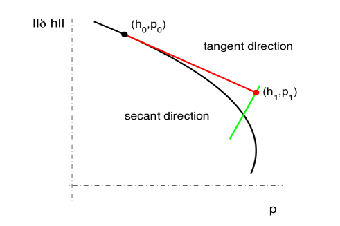
Fig. 2: Scheme of a continuation step using the tangent predictor - secant corrector method.

First, we describe a continuation step as sketched in Fig. 2. One starts at point $(h_{0},p_{0})$ representing a steady state $h_{0}$ at parameter value $p_{0}$. Differentiating (24) one obtains the tangent direction $(\delta u_{t},\delta p_{t})$ of the continuing branch at the point $(h_{0},p_{0})$ as solution of the system

$$\mathbf{J_{0}}u_{t}=-D_{p}F(h_{0},x,p_{0})\delta p_{t}$$ (25)

where $\mathbf{J_{0}}=D_{h}F(h_{0},x,p_{0})$ is the Jacobian. The $(\delta u_{t},\delta p_{t})$ solution is entirely determined by fixing the amplitude of $\delta p_{t}$. This is done by finding the maximal amplitude of $p_{t}$ such that

$$||F(h_{0}+\delta u_{t},x,p_{0}+\delta p_{t})||<\epsilon_{t}||h_{0}||$$ (26)

to stay close to the steady state branch. Typically we take $10^{-3}<\epsilon_{t}<10^{-1}$. We denote this intermediate point by $(h_{1},p_{1})$ with

$$h_{1} = h_{0}+\delta u_{t}$$ (27)

$$p_{1} = p_{0}+\delta p_{t}.$$ (28)

The sign of $\delta p_{t}$ remains to be chosen. It only changes at saddle-node bifurcations. In the $(p,f(p))$ plane the passing of a saddle-node bifurcation is characterized by a sign change of $f^{\prime}(p)$ and an increase of $|f^{\prime}(p)|$ before reaching the bifurcation. If both conditions are fulfilled the sign of $\delta p_{t}$ has to be changed.

Next, one uses Newton’s method to solve Eq. (24) close to $(h_{1},p_{1})$. The secant is taken orthogonal to the tangent $(\delta u_{t},\delta p_{t})$ to be able to follow the branch even in the neighborhood of a turning point. For the Newton iteration step that starts from $(h_{k},p_{k})$ the condition reads

$$\mathbf{J_{k}}u_{k+1} = -F(h_{k},x,p_{k})-D_{p}F(h_{k},x,p_{k})\delta p_{k}$$ (29)

$$\left<u_{t},\delta u_{k}\right> = 0$$ (30)

$$h_{k+1} = h_{k}+\delta u_{k}$$ (31)

$$p_{k+1} = p_{k}+\delta p_{k}$$ (32)

where $\mathbf{J_{k}}=D_{h}F(h_{k},x,p_{k})$ and $\delta u_{k},\delta p_{k}$ are the unknowns at step $k+1$. Eq. (29) and the orthogonality condition (30) written as matrix equation are

$$\left[\begin{array}[]{cc}\mathbf{J_{k}}&D_{p}F(u_{k},x,p_{k})\\ u_{t}&0\end{array}\right]\left[\begin{array}[]{c}\delta u_{k}\\ \delta p_{k}\end{array}\right] = \left[\begin{array}[]{c}-F(u_{k},x,p_{k})\\ 0\end{array}\right]$$ (39)

$$\mathbf{N}\left[\begin{array}[]{c}\delta u_{k}\\ \delta p_{k}\end{array}\right] = \left[\begin{array}[]{c}-F(u_{k},x,p_{k})\\ 0\end{array}\right].$$ (44)

One clearly sees, that the continuation step requires inversions of the Jacobian matrix $\mathbf{J}$ (tangent predictor) and of the matrix $\mathbf{N}$ (Newton corrector steps). Except at bifurcation points, systems are invertible in the space $E_{0}$. As above, the restriction to $E_{0}$ is ensured during the Krylov reduction (see appendix A).

4.3 Computation of the tangent predictor

The Cayley-Krylov reduction of (25) leads to

$$V_{m}\mathbf{J_{m}}V_{m}^{t}u_{t}=-b\delta p_{t}=-D_{p}F(h_{0},x,p_{0})\delta p_{t}.$$ (45)

where ${V_{m}}$ is the Krylov basis consisting of $m$ vectors in $E_{0}$. It is constructed by letting the operator $\mathbf{C}=(\mathbf{J}-c\mathbf{I})^{-1}$ act on the vector $b=D_{p}F(u_{0},p_{0})$. The choice of the scalar $c$ follows the same rules as in the time-stepping (appendix A). Using the QR-method the spectrum of the reduced $m\times m$ Jacobian is obtained:

$$\mathbf{J}_{m}=\mathbf{P_{m}}\mathbf{D_{m}}\mathbf{P_{m}^{-1}}.$$ (46)

For the inversion we distinguish two cases: (i) if the kernel contains a non-zero eigenvector $v_{0}$, then the pair $(v_{0},0)$ is the solution of the problem; (ii) otherwise we perform the inversion and the solution is given by

$$u_{t}=-V_{m}\mathbf{{P_{m}D_{m}}^{-1}P_{m}^{-1}}V_{m}^{t}b\delta p_{t}.$$ (47)

In this way one is able to detect bifurcation points and ensures that the continuation works well at turning points.

4.4 Computation of the secant corrector

To perform one Newton step (44), the same method as in the previous paragraph is applied to the matrix $\mathbf{N}$ instead of $\mathbf{J}_{m}$. Note that, because of the secant direction requirement (30) the matrix $\mathbf{N}$ is invertible in $E_{0}$ even close to a bifurcation point.

As both, tangent predictor and secant corrector step, need an ILU-factorization, it is the most important numerical task in the continuation algorithm (as for the time-stepping algorithm).

4.5 Bifurcation analysis and stability analysis

Because the rightmost spectrum of the Jacobian is known we are as well able to assess the stability of solutions. Furthermore, during the tangent predictor step one is able to detect the presence of bifurcations. The direction of the bifurcating branch may be deducted from the eigen-directions of the kernel. Although, the rightmost spectrum is normally well evaluated it may occur that the rightmost eigenvalue $\lambda_{\rm max}$ is not in the Krylov space (see appendix A). Furthermore, the accuracy of the estimation of the rightmost eigenvalues is only about $10^{-3}$. To determine the bifurcation point more accurately one has to apply a different algorithm as, e.g., a block Arnoldi method [74] adapted to the Cayley-Arnoldi algorithm. In the following the developed algorithms are used to study important questions related to the dewetting of a thin film (Section 5) and the depinning of a drop (Section 6).

5 Short-time dynamics and coarsening for dewetting thin films

The dewetting of a thin film can be initiated by two different mechanisms: Either via a surface instability (spinodal dewetting) or by heterogeneous nucleation at finite size defects [24, 83, 75, 84]. Dewetting of metastable films can only be initiated by nucleation, i.e., by finite disturbances larger than a critical threshold given by an unstable steady state. For linearly unstable films, there exists a critical wavelength $\lambda_{c}=2\pi/k_{c}$. Any disturbance associated to a wavelength $\lambda>\lambda_{c}$ grows exponentially in time with a growth rate $\beta=-m(h_{0})k^{2}(k^{2}-k_{c}^{2})$. The resulting short-time dewetting structure consists of a drop, hole or labyrinthine pattern. Its characteristic scale corresponds to the wave length $\lambda_{m}=\sqrt{2}\lambda_{c}$ of the fastest growing linear mode. However, whether this linear instability is the dominant mechanism depends on the character of the primary bifurcation: Deep inside the linearly unstable regime it is supercritical and the film necessarily develops the surface instability. However, closer to the metastable region the primary bifurcation is subcritical. Then threshold solutions are present. They offer as second pathway of evolution a nucleation process as in the metastable regime [95, 97, 83, 3]. The latter normally dominates if the growth rate of the threshold solution is much larger than the largest growth rate of the linear instability $\beta_{m}$. Details of the dewetting process then strongly depend on experimental conditions (amount of defects, roughness, noise). When nucleation dominates one expects larger drops or holes that are randomly distributed. Here we investigate (i) the dominance of either instability- or nucleation-triggered dewetting in the linear unstable thickness region in the 2d case; and (ii) quadratic and hexagonal steady state solutions in the 2d case and the character of their primary bifurcations. The short-time dewetting dynamics is followed by a very slow coarsening process resulting eventually in a single drop coexisting with the precursor film. The coarsening advances via a cascade of two- (and three-)drop mergers based on two mechanisms related to a volume and a translation mode, respectively [33, 45]. In the volume mode all liquid flows through the precursor film and the centers of mass of the drops do not move. In the translation mode the entire drops approach each other and merge. The stabilization of the two modes by a substrate heterogeneity is discussed in Ref. [86]. It implies that during coarsening the major part of the dynamics occurs in the contact line regions. Because the motion is related to the Goldstone mode of translational invariance for a single liquid front [45] the corresponding eigenvalues are close to zero. Note that a coarsening step can be interpreted as a heteroclinic connection between unstable steady states.

5.1 The one-dimensional case

We use the 1d case with disjoining pressure (I) to compare our results to the literature [97]. The initial profile is a flat film with a small localized defect at the center. The Cayley transform is used with a regular mesh with $N=1600$ for a domain size $\ell=16\lambda_{m}$.

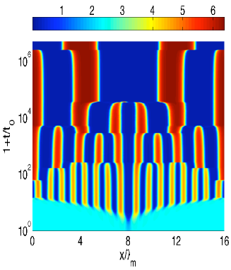
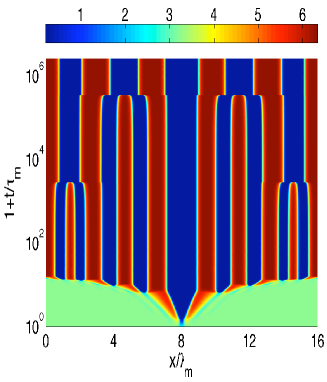
(a)                                                        (b)

Fig. 3: Space-time contour plots for the time evolution of the film thickness profile $h$ during dewetting in (a) the surface-instability-dominated regime ($H=2.4$) and (b) the nucleation-dominated regime ($H=3.2$). The initial film is linearly unstable in both cases. We consider the disjoining pressure (I) with $G=0.05$ and the mobility function $m(h)=(h^{3}-\ln(0.1))^{3}$ (for details see [97]). The domain size is $16\lambda_{m}$ and the initial profile is a flat film with a single defect: $h_{0}=H\left(1-0.1\cosh(5x/\lambda_{m})^{-2}\right)$. The parameters agree with the ones used in Fig. 14 of [97].

(a)
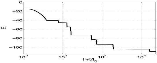
(b)

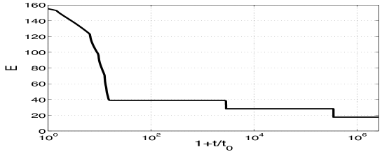
Fig. 4: Change of the energy $E$ with time for dewetting at (a) $H=2.4$ and (b) $H=3.2$ corresponding to time evolutions given in Fig. 3. The energy $E$ is defined as in [97]: $E=(1/L)\int[(\partial_{x}h)^{2}/2+f(h)]dx$ with the local energy $f(h)=-\int\Pi(h)dh$.

Figures 3(a) and (b) give space-time plots of the long-time evolution in the cases of dominating surface instability ($H=2.4$) and nucleation ($H=3.2$), respectively. In Fig. 3(a) the initial growth ($t\leq 15\tau_{m})$ results in a regular array of 16 drops of distance $\lambda_{m}$. The profile and the evolution of the norm and the relative energy (Fig. 4) do well agree with [97] (their figures 14(a) and 16(a)). In Fig. 3(b) the growth of the hole resulting from the finite disturbance is faster than the surface instability. Further holes are subsequently nucleated by secondary nucleation events close to the primary hole. The resulting short-time structure consists of fewer larger drops than in the surface instability regime. The initial ’rupture’ phase in 4(b) is in good agreement with Fig. 16(b) of [97].

Our method allows us to study the long-time coarsening far beyond the results of, e.g., [96, 86]. In Fig. 3 one can identify both coarsening modes in agreement with Refs. [33, 45]. The merging of drops does not occur continuously slow but starts extremely slow and culminates very fast. In consequence, the evolution of the energy (Fig. 4) shows long plateaus connected by ’jumps’. Our adaptive time-step method copes very well with this combination of slow and fast dynamics.

The coarsening process in the nucleation case (Fig. 3(b)) is slower than in the surface instability case and proceeds mainly via the mass transfer mode. Finally, two [five] drops remain in the surface instability [nucleation] case. In principle, coarsening should continue, but the evolution becomes so slow that we reach the limit of numerical accuracy, i.e., the eigenvalues related to the coarsening modes become smaller than the numerical accuracy. In particular, for leading eigenvalues smaller than $10^{-7}$, the numerical noise is not negligible and we are not able to observe the next coarsening step.

We conclude that the developed algorithm is well suited to study the short- and long-time behavior in the 1d case. In particular, the short-time evolution agrees well with results obtained using a semi-implicit scheme with a constant time-step [97]. In contrast, here the time-step varies by 6 orders of magnitude allowing us to study the long-time coarsening.

5.2 The two-dimensional case

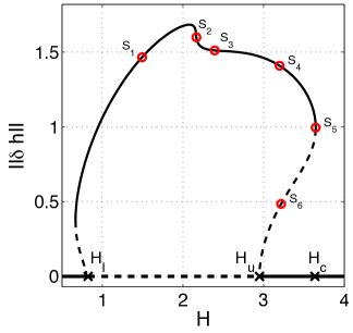
(a) (b)

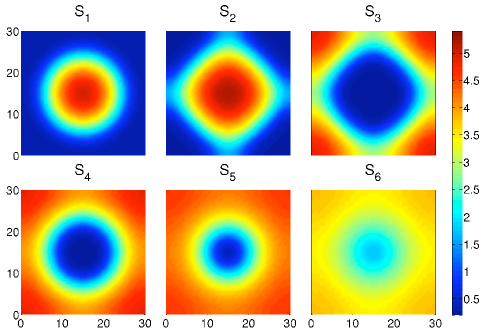
Fig. 5: (a) Bifurcation diagram for a 2d square array of drops/holes on a horizontal homogeneous substrate. The domain size is $30\times 30$. Shown is the $L^{2}$ norm $||\delta h||$ as a function of the mean height of liquid $H$. The steady state solutions may be linearly stable (solid line) or unstable (dashed line). (b) Contour plots of steady state solutions indicated by circles in the bifurcation diagram. With the exception of the control parameter $H$, all parameters are as given in Section 5.2.

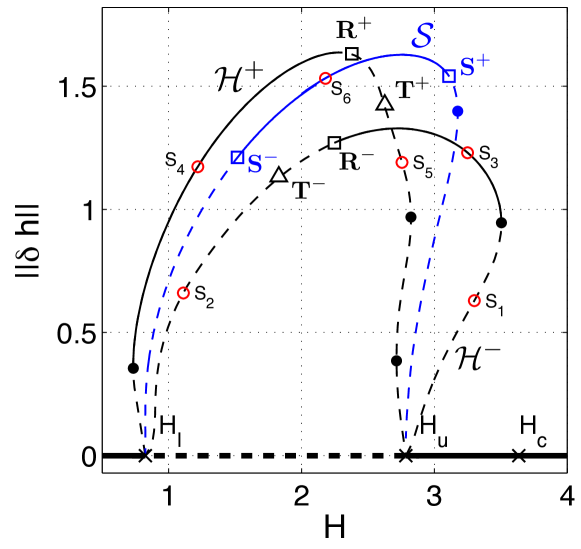
Fig. 6: Bifurcation diagram for a 2d hexagonal array of drops/holes on a horizontal homogeneous substrate. The domain size is $30\times 30\sqrt{3}$. Shown is the $L^{2}$ norm $||\delta h||$ as a function of the mean height of liquid $H$. Black lines correspond to the branches of hexagons ($\cal{H}^{+}$ and $\cal{H}^{-}$), whereas the blue line corresponds to the branch of stripes ($\cal{S}$). The steady state solutions may be linearly stable (solid line) or unstable (dashed line). The dots, squares and triangles represent secondary bifurcations as explained in the main text. The hollow circles indicate solutions that are displayed in Fig. 7. The remaining parameters are as given in Section 5.2.

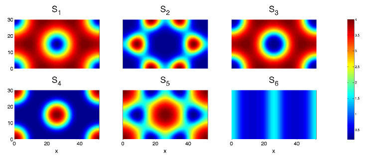
Fig. 7: Contour plots of steady state solutions indicated by hollow circles in the bifurcation diagram of Fig. 6. In particular, the upper row gives three hole solutions from the $\cal{H}^{-}$ branch ($S_{1}$ to $S_{3}$), whereas the lower row gives two drop solutions from the $\cal{H}^{-}$ branch ($S_{4}$ and $S_{5}$) and a typical stripe solution ($S_{6}$). Of the shown solutions only $S_{3}$, $S_{4}$ and $S_{6}$ are linearly stable.

After having shown the reliability of our algorithm for 1d dewetting, we next employ it to study the 2d case. The above discussion of the linear stability still applies. In particular, the fastest growing wavelength $\lambda_{m}$ and corresponding growth rate $\beta_{m}$ are identical. However, in contrast to the 1d case, 2d patterns involve two wave vectors $\mathbf{k_{1}}$ and $\mathbf{k_{2}}$ that can lead to a variety of periodic steady state patterns [19]. Here, we track square and hexagonal patterns by imposing a periodic $30\times 30$ square and a $30\times 30\sqrt{3}$ rectangular domain, respectively. Choosing the mean film thickness $H$ as control parameter we obtain the bifurcation diagrams in Figs. 5(a) and 6(a), respectively. Note that the finite domain size results in critical film thicknesses different from the one for an infinite domain. In particular, one finds $H_{u}=2.79$ for the upper limit instead of $H_{c}=3.63$ expected for an infinite domain. Fig. 5(a) shows that for the square pattern at $H_{u}$ an (unstable) subcritical branch bifurcates from the trivial one. It stabilizes and turns towards smaller $H$ at a saddle-node bifurcation at $H_{\mathrm{sn}}\simeq H_{c}$. In consequence, for $H_{u}<H<H_{sn}$ the flat film is metastable and can only dewet via nucleation that allows it to pass the unstable threshold solution. In a similar way, the lower critical thickness $H_{l}=0.825$ differs slightly from the one for an infinite domain ($H_{cl}=0.747$, not shown in the bifurcation diagrams).All steady state profiles above $H\approx 2.2$ correspond to hole patterns (see Fig. 5(b)). Further decreasing $H$, a morphological transition occurs (related to the steep variation in the norm at $H\simeq 2.2$) via a state of a rotated (by $\pi/4$, see states $S_{2}$ in Fig. 5(b)) checkerboard pattern to drop patterns that always prevail at smaller $H$. At another saddle-node, the branch turns and becomes unstable again before subcritically joining the flat film state at $H_{1}=0.84$.

Fig. 6 shows branches of hexagonal symmetry that bifurcate from the trivial solution. It does as well give the secondary bifurcations. Note, however, that here we do not show the secondary branches although they are discussed in passing in the following. In contrast to the square patterns in Fig.5, the branches of hexagonal patterns do not display a transition between drops and holes at finite amplitude. However, at each of the two bifurcation points ($\bf H_{l}$ and $\bf H_{u}$) the hexagonal branch crosses the trivial flat film solution branch in a transcritical bifurcation. In the representation of Fig.  6 this corresponds to two families of hexagons that seem to emerge at each bifurcation point. Ones of them consist of a hexagonal array of drops (see states $S_{4}$ and $S_{5}$ in Fig. 7) and is equivalent to the $\cal{H}^{+}$ branch discussed in [21]. The other one represents a hexagonal array of holes (states $S_{1}$ to $S_{3}$ in Fig. 7) and corresponds to the $\cal{H}^{-}$ branch [21].

Each of these branches connects the two bifurcation points $\bf H_{l}$ and $\bf H_{u}$. Additionally to the branches of hexagons, a branch of stripe solutions $\cal{S}$ appears through a supercritical pitchfork bifurcation at $\bf H_{l}$ and ends at a subcritical pitchfork bifurcation at $\bf H_{u}$. All these branches are unstable near the primary bifurcation as expected for the generic case of bifurcations with hexagonal symmetry [21].

The branches gain and loose stability through a number of secondary bifurcations in a scenario that is similar to one described in [15]: The branch $\bf\cal{H}^{+}$ that emerges at $\bf H_{l}$ first continues towards smaller $H$, then turns and gains stability at a saddle-node bifurcation. It continues towards larger $H$ and loses its stability again at a transcritical bifurcation (point $\bf R^{+}$ in Fig. 6). Note that it undergoes another two saddle-node bifurcations before approaching $\bf H_{u}$. The branch that crosses at $\bf R^{+}$ has rectangular symmetry; one side connects to the bifurcation point $\bf S^{+}$ on the branch of stripe solutions ($\cal{S}$); the other one crosses the $\cal{H}^{-}$ branch transcritically at $\bf R^{-}$ before ending at $\bf S^{-}$ on the branch of stripe solutions.

A similar scenario occurs for the branch $\cal{H}^{-}$ when starting at the transcritical bifurcation at $\bf H_{u}$: It continues towards larger $H$, then turns and gains stability at a saddle-node bifurcation. It continues towards smaller $H$ and loses its stability at $\bf R^{-}$. Finally, the branch of stripe solutions $\cal{S}$ that emerges at $H_{l}$ gains stability at $\bf S^{+}$ and loses it again at $\bf S^{-}$. The saddle-node bifurcation at larger $H$ does not change its stability.

This introduces all bifurcations necessary to understand the stability of the primary branches. Note however, that there exist further secondary bifurcations ($\bf T^{+}$ and $\bf T^{-}$ in Fig. 6) involving a branch of triangular solutions. As discussed in [15], this branch connects the two hexagonal branches $\cal{H}^{+}$ and $\cal{H}^{-}$.

Although the bifurcation analysis is very instructive for a small domain, it does not allow one to directly predict which mechanism dominates 2d dewetting for larger system sizes. To study this question we employ our time-stepping algorithm. The use of different initial disturbances allows one to discuss the prevalence of either dewetting by nucleation or by surface instability for linearly unstable films: We chose an radially symmetric defect of profile $h(r)$ (identical to the $h(x)$ in the 1d case) that shall compete with the surface instability that emerges from an initial film roughness. Without initial roughness one finds that the short-time evolution conserves the radial symmetry until the boundaries of the square box are felt. In the instability dominated case ($H=2.4$, Fig. 8(a)) the distance between rings corresponds as expected to $\lambda_{m}$, whereas in the nucleation-dominated regime ($H=3.2$, Fig. 8(b)) it is roughly $2\lambda_{m}$ and the boundary is felt earlier. After the ring formation during the short-time evolution, the rings break and coarsening sets in. In the radially symmetric part coarsening starts at the center and proceeds through a cascade of ring contractions.

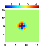
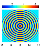
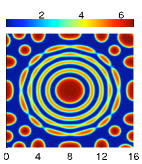
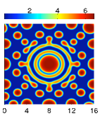
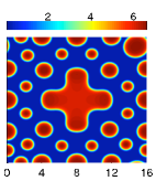
(a)     $5.57$ $15.4$ $122$ $259$ $467$         

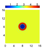
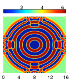
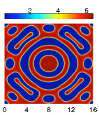
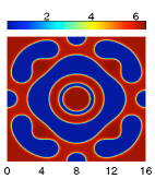
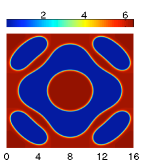
(b)     $5.60$ $14.5$ $54.4$ $140$ $326$

Fig. 8: Snapshots from the evolution of dewetting thin films. The initial condition corresponds to a flat film with a central defect: $h_{0}=H\left(1-0.1\cosh(5r/\lambda_{m})^{-2}\right)$ in the (a) surface-instability-dominated regime at $H=2.4$ and (b) in the nucleation-dominated regime at $H=3.2$. The domain size is $16\lambda_{m}\times 16\lambda_{m}$ and we use periodic boundary conditions. The time is indicated below the individual panels in units of $\tau_{m}$. The remaining conditions are as in Fig. 3.

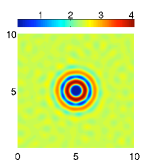
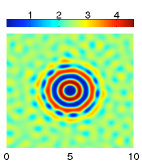
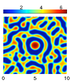
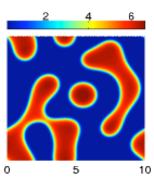
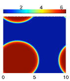
(a)     $4.92$ $6.19$ $15.7\cdot 10$ $118$ $3.25\cdot 10^{4}$         

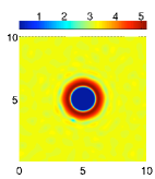
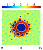
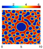
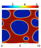
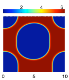
(b)     $4.29$ $5.69$ $10.4$ $120$ $1.14\cdot 10^{3}$         

Fig. 9: Snapshots from the evolution of dewetting thin films in the (a) surface-instability-dominated regime at $H=2.4$ and (b) in the nucleation-dominated regime at $H=3.2$. The initial condition is as in Fig. 8 with an added roughness of 0.1% of $H$. The domain size is $10\lambda_{m}\times 10\lambda_{m}$ and all other settings are as in Fig. 8.

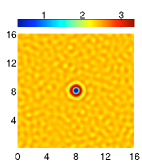
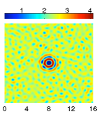
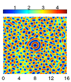
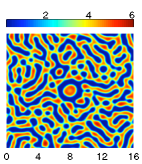
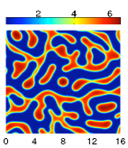
(a)     $3.42$ $4.84$ $6.51$ $12.5$ $34.1$         

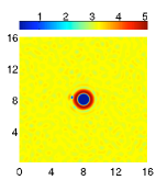
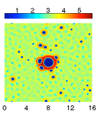
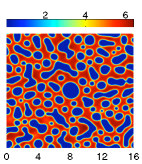
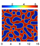
(b)     $3.03$ $4.09$ $5.21$ $10.7$ $32.0$         

Fig. 10: Snapshots from the evolution of dewetting thin films for (a) $H=2.4$ and (b) $H=3.2$. The initial condition corresponds to the one in Fig. 8 with an added roughness of of 1.0% of $H$. The domain size is $16\lambda_{m}\times 16\lambda_{m}$ and all other settings are as in Fig. 8.

The result shows that the numerical noise is small enough to not break the radial symmetry during the time integration. Adding, however, an initial roughness the symmetry is rapidly destroyed (see below). This explains why normally in dewetting experiments with very thin films that are affected by thermal noise and other tiny perturbations no such regular structures are observed. However, recent experiments with electrically destabilized thicker films (less prone to noise) show regular ring structures when an inhomogeneous electrical field is applied in such a way that it plays the role of our initial radially symmetric defect (see Figs. 2 and  4 of Ref. [18]).

To determine the influence of noise of the relative importance of nucleation and surface instability we perform several simulations using different initial film roughness $\zeta$. In particular, we add a roughness of $\zeta=0.1$% (Fig. 9) and $\zeta=1$% (Fig. 10) of the mean film thickness. The larger $\zeta$ becomes, the less time has the radial structure to evolve because the roughness ’accelerates’ the isotropic surface instability. For small $\zeta=0.1$% the radial symmetry is appreciable quite some time even into coarsening (Fig. 9). However, coarsening eventually ’washes out’ any memory of the initial defects. In particular, for $H=2.4$ the second ring is still complete (at $t=4.92$), but already the next depression is not radially symmetric but resembles a ring-like assembly of holes (at $t=6.19$). For $H=3.2$, already the depression outside the first ring emerges as a circular hole pattern, i.e., as a typical secondary nucleation pattern (cf. [3]). In both cases the initial defect has no further influence on the structure. The remaining area is covered by typical spinodal structures. For the stronger initial roughness ($\zeta=1$%, Fig. 10) the initial defect is of minor influence, i.e., the central radial structure only dominates during a very short time (till about $t=3\dots 4$) and is later homogenized through coarsening. Everywhere else the surface instability dominates.

6 Depinning of a drop on a heterogeneous substrate

The second problem we focus on is the depinning of drops. If a lateral force is applied on films/drops on a homogeneous substrate [$P\neq 0$ in Eq. (2)], one only finds traveling surface waves or sliding drops [96, 89]. No steady-state solutions exist, except for the flat film. On a heterogeneous substrate, however, the heterogeneity (e.g., chemical or topographical defect) can pin a drop. Here, we consider wettability defects in the form of stripes, i.e., we use disjoining pressure (III) that is modulated in the $x$-direction (cf. Eq. (5)). The resulting wettability profile $\xi(x)$ is presented in the lower panels of Fig. 13. The parameter $\epsilon$ represents the amplitude of the heterogeneity, i.e., the wettability contrast. If $\epsilon>0$ [$\epsilon<0$] the defect is less [more] wettable than the surrounding substrate, i.e., the defect is hydrophobic [hydrophilic].

When the lateral driving is increased the pinned drops are deformed and their center of mass slightly shifts until at a critical driving $P_{c}$ the drop depins. The analysis of the steady states and the depinning bifurcation is tackled using the continuation approach developed above in Section 4. In the 1d case, results are already available: In Ref. [92, 91] the continuation package AUTO [28] and an explicit time-stepping algorithm with adaptive time-step were used. We employ this case in Section 6.1 to validate our continuation code. As the results for identical parameters are identical to the ones of Ref. [92, 91], we here present results for larger drops. In Section 6.2 we explore the 2d case which can not be treated using AUTO because the governing equations are not equivalent to an ODE system.

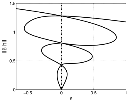
Fig. 11: Bifurcation diagram for 1d steady drop solutions on an horizontal heterogeneous substrate ($P=0$). Shown is the $L^{2}$-norm $||\delta h||$ versus the defect strength $\epsilon$. The used disjoining pressure (III) is given by Eq. (5) with $b=0.1$; and the domain size is $L=50$.

6.1 The one-dimensional case

For a homogeneous substrate without lateral driving ($\epsilon=0$ and $P=0$), the critical wavelength for a film of thickness $H=1.5$ is $\lambda_{c}\simeq 15$, i.e., for a domain size of $L=50$ there exist at least steady states containing one, two or three drops. They bifurcate from the flat film at $n\lambda_{c}$ with $n=1,2,3$, respectively. If the primary bifurcation is subcritical there might be more solutions (cf. Ref. [90]).

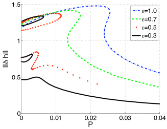
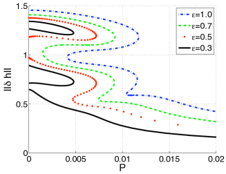
(a)                                                        (b)

Fig. 12: Bifurcation diagrams for families of pinned 1d steady solutions representing one-, two- and three-drop states for (a) hydrophobic and (b) hydrophilic defects of various strength $\epsilon$ as given in the legend. Shown is the $L^{2}$ norm $||\delta h||$ in dependence of the lateral driving force $P$ The remaining parameters are as in Fig. 11.

To determine the various steady-state solutions for a heterogeneous substrate without lateral driving we use continuation when varying the heterogeneity strength $\epsilon$ for a heterogeneity period equal to the domain size (Fig. 11). Branches of steady-state solutions cross the axis $\epsilon=0$ three times, corresponding to the one-, two- and three-drop solution for a homogeneous substrate. For a strong heterogeneity ($|\epsilon|$ large) only the single drop solution remains that is the most interesting solution for a study of depinning. However, for smaller $|\epsilon|$ up to seven steady states can exist corresponding to various stable and unstable one-, two, and three-drop equilibria. As Ref. [92] studies a smaller domain ($L=25$) their Fig. 6 only shows one crossing of the axis $\epsilon=0$. Studying the stability of the equilibria one finds that only the uppermost branch corresponds to stable solutions. All other branches terminate in saddle-node bifurcations.

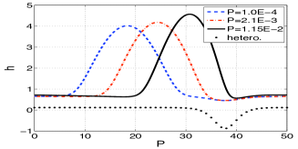
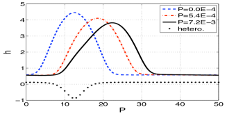
(a)                                                        (b)

Fig. 13: Selected steady drop profiles on a heterogeneous substrate for different driving forces $P$ as given in the legend. Shown are (a) the hydrophobic case with defect strength $\epsilon=0.5$, and (b) the hydrophilic case with $\epsilon=-0.5$. The respective solid line represents the profile at depinning. The lower part of the panels gives the profile $\xi(x)$ of the heterogeneity.

Next, all steady-state branches are tracked when increasing the lateral driving force $P$ from zero for various fixed $\epsilon$. Bifurcation diagrams and selected profiles of pinned drops are given in Figs. 12 and 13, respectively. The various branches found for $P=0$ continue to exist for small driving as ’pinned solutions’. However, at critical values of the driving most ’annihilate’ each other. Physically speaking, the heterogeneity can not retain the drops any more and they start to slide, i.e., they depin. Beyond a critical value $P_{c}$ no steady drop does exist as even the stable single drop depins (Fig. 12). The bifurcation at $P_{c}$ is a sniper (Saddle Node Infinite PERiod) bifurcation. At $P_{c}$ a branch of space- and time-periodic solutions emerges (not shown) that corresponds to drops sliding on the heterogeneous substrate. The temporal period diverges as one approaches $P_{c}$ from above and the drop motion resembles stick-slip behavior (cf. Refs. [92, 91]. The obtained results indicate that our continuation algorithm is well capable to follow stable and unstable steady states in the 1d case. The saddle-node bifurcation has been well detected and as expected no numerical stability problems have been encountered near the bifurcation. Next, the continuation algorithm has to prove its capabilities in the 2d case.

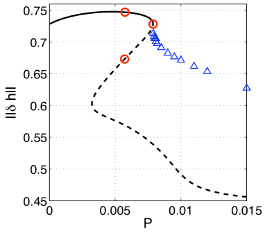
Fig. 14: Bifurcation diagram for the depinning of 2d drops from a hydrophobic line defect given by Eq. (5) with $\epsilon=0.3$. Shown is the $L^{2}$ norm $||\delta h||$ in dependence of the driving force $P$ for steady state solutions (solid line). For depinned sliding drops the time-averaged norm is given (symbols ’$\Delta$’). The domain size is $40\times 40$. The circles indicate the steady states represented in Fig. 15. All other parameters are as in Section 6.1

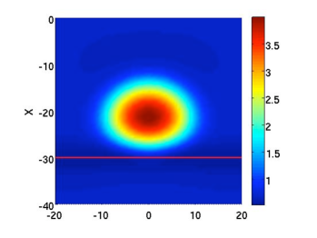
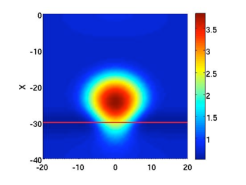
y                                                       y
                          (a)                                                      (b)

Fig. 15: Shown are contours of the pinned (a) stable and (b) unstable steady drop solutions at $P=5.68\cdot 10^{-3}$ (leftmost circles in Fig. 14). The thin horizontal line marks the maximum of the heterogeneity. The remaining parameters are as in Fig. 14.

6.2 The two-dimensional case

In the 2d case we consider stripe-like wettability defects. In particular, we employ an $x$-dependent heterogeneity profile and choose the lateral driving force $P$ as well in $x$-direction. In this way a hydrophobic stripe ($\epsilon>0$) blocks a drop at its front end whereas a hydrophilic one ($\epsilon<0$) holds it at the back end. Fig. 14 presents the bifurcation diagram for $\epsilon=0.3$ obtained when continuing the steady single stable drop solution for increasing $P$. Stable (unstable) states are given as solid (dashed) lines. The stable blocked drop increases its norm with increasing driving as it is ’pressed’ against the defect. The drop finally depins at a saddle-node bifurcation ($P_{c}\approx 0.003$) where the stable branch turns and loses stability. Time simulations beyond depinning show a typical stick-slip motion of drops with a period that diverges when the bifurcation is approached from above. The time averaged norm for selected values of $P$ is indicted by triangles in Fig. 14. The results indicate that depinning occurs via a sniper bifurcation.

Examples of steady stable and unstable drop profiles are given in Figs. 15(a) and (b), respectively. The stable drop sits behind the line of minimal wettability. As it is squeezed against the defect by the driving force it has an oval shape. In contrast, the unstable drop, has a ’forward protrusion’ that crosses over the minimum of wettability. This solution represents a depinning threshold for $P<P_{c}$, i.e., adding a small perturbation will either let the drop retract its advancing protrusion to again settle behind the defect or trigger a depinning event that sends the drop sliding down to the next defect where it is pinned again. For a more detailed analysis of the depinning process in 2d see Ref. [4].

Finally, let us come back to the computational scheme. Apart from the increase in the system size $N$, in the 2d case one encounters a new difficulty related to the translation symmetry in $y$-direction. It implies that for each solution there exist a continuum of solutions obtained by translation in $y$-direction that has to be avoided by the continuation algorithm. Neglecting numerical noise, the solutions possess a left-right reflection symmetry $y\rightarrow-y$ (Fig. 15). Therefore, the Jacobian is an equivariant operator for this left-right reflection. Thus, the action of the Jacobian on left-right symmetric vectors results in vectors with the same symmetry. This effectively excludes any translation in the $y$-direction. However, when the solution is close to the trivial flat film state even small numerical noise becomes relevant and the leading eigenvalues are very small as well. In the above numerical example we observe related problems for large driving at $P>0.1$ when the steady solution corresponds to very shallow rivulet. The continuation algorithm might then stay on the orbit of solutions related by translation. The problem can be easily overcome by fixing the maximum at a particular point, although, this might cause problems in situations where various maxima may coexist. To avoid any ambiguity, we use a similar technique as for the problem of mass conservation: in the Krylov step we project the basis vectors orthogonally to the translation mode $\partial_{y}h_{0}$. This does not change the structure of the algorithm and is performed at negligible cost (see app. A).

7 Conclusion

We have presented (i) a time integration scheme based on exponential propagation and (ii) a continuation algorithm employing the Cayley transform for the highly non-linear thin film equations. These equations contain differential operators till fourth order. To avoid severe stability restrictions on the time-step, a linear term may be treated implicitly. However, for the thin film equations the difficulty is to find a relevant linear operator. In consequence we use the Jacobian matrix at each time-step. In this framework, an exponential propagation scheme is more efficient than a semi-implicit scheme [39, 98]. The method is based on an exact solution of the linear problem for each time-step and involves the determination of the exponential of a matrix. To do this in an economic way, the linear operators may be reduced to small Krylov subspaces. However, for the thin film equation we need a dimension of the Krylov subspaces of about 100 – much larger than necessary for problems involving only a second order operator [31]. For better convergence of the Krylov reduction, we have coupled the Arnoldi algorithm with the Cayley transform that is performed using an ILU-factorization. In consequence, this Cayley-Arnoldi method allows us to take larger time-steps and, furthermore, well estimates the leading eigenvalue. This facilitates an effective adaption of the time-step to the changing characteristic time scale of the dynamics. This has led to a major improvement in simulations of one- and two-dimensional thin film dynamics that involve multiple time scales as, e.g., coarsening dynamics for dewetting films or the stick-slip motion close to depinning transitions.

We have also developed an algorithm for the continuation (or path-following) of steady states that is based on the tangent predictor - secant corrector scheme. Both tasks – time stepping and continuation – can be performed using the same Cayley-Arnoldi algorithm. The advantage of this approach is the possibility to perform all tasks arising in a bifurcation analysis simultaneously. This includes the computation of the kernel of the Jacobian to detect bifurcations and the stability analysis of the steady states. The developed algorithms have been used to study the bifurcation structure and time evolution of (i) dewetting thin films and (ii) depinning drops for physically two- and three-dimensional settings, that correspond to 1d and 2d thin film equations, respectively.

For the dewetting film we have investigated different pathways for the initial ’rupture’, i.e., the short-time evolution. The focus has been on the competition of the surface instability and the nucleation at defects. The long-time coarsening dynamics has as well been studied. For the 1d case, we could follow the coarsening process till $10^{6}\tau_{m}$ where $\tau_{m}$ is the characteristic time of the surface instability. In the two-dimensional case, we have found that the short-time dewetting process induced by a radially symmetric finite defect conserves the radial symmetry until disturbed by the boundaries of the square domain. This indicates the very small influence of round-off errors in our algorithm. The coarsening then proceeds via a cascade of ring contractions. However due to the importance of thermal fluctuations such regular structures are normally not observed in dewetting experiments with very thin films. However, they are observed for thicker dielectric films in a capacitor when an inhomogeneous electrical field plays the role of the finite defect [18]. Adding noise to the initial conditions we recover the ’classical’ dewetting structures. Using the Cayley-Arnoldi method for a system size of about $10\lambda_{m}\times 10\lambda_{m}$, one is able to simulate the coarsening dynamics till reaching a single drop, i.e., the globally stable solution (Fig. 9). Beside the time evolution we have employed continuation to study 2d steady state solutions corresponding to square and hexagonal arrangements of drops or holes.

Second, we have studied the depinning of ridges (1d case) and drops (2d case) from substrate heterogeneities. Pinned steady solutions have been followed using our path-following algorithm. In particular, we have used as continuation parameters the wettability contrast and the lateral driving force. In the 1d case we have successfully reproduced results obtained in Refs. [92, 91] using the package AUTO [28]. We have as well tracked 2d stable and unstable steady drop solutions. This has been supplemented by a study of the evolution of time-dependent solutions beyond depinning. This has led us to the conclusion that in the 2d case depinning occurs as in the 1d case via a sniper bifurcation and that beyond (but close to) the bifurcation the sliding drops show stick-slip behavior.

Although our approach improves the time integration and path-following for thin film equations, the employed constant equidistant finite difference spatial discretization remains very basic. The weakness of such a regular discretization appears, for instance, when tracking large drops pinned at hydrophobic defects. For increasing driving force the stable drop becomes strongly localized at the defect. The unstable solution for the same driving force is very close to the stable one as already observed in the 1d case for large drops (Fig. 29 of Ref. [92]). To clearly distinguish the two solutions numerically a higher accuracy is required. This can be achieved using an adaptive mesh. In our particular system, for instance, the continuation procedure applied to a drop on a $50\times 50$ square domain breaks down near the depinning bifurcation. This accuracy problem is similar to the one encountered in the last stages of coarsening in Section 5.1 where a mesh refinement near the drop edges would be beneficial.

We have restricted our study to thin film equations that describe films and drops on partially wettable homogeneous and heterogeneous substrates. Beside the curvature pressure, the disjoining pressure has been the only term resulting from the underlying free energy. However, the method can be applied to various thin film systems involving other contributions to the free energy. This includes, for instance, thin films of dielectric liquid in a capacitor [56, 100, 2], heated thin films [64, 11, 90], films with an effective thickness dependent surface tension caused by high-frequency vibration [49, 94] and film flows in a time-dependent ratchet potential [43]. The algorithms can also be applied to multilayer problems in the long-wave framework like, for instance, in bilayer dewetting [68, 1, 69] or to systems involving a single thin film equation coupled to a (reaction-)diffusion equation for a reactive [23, 65] or non-reactive [41, 54] surfactant or adsorbate at the substrate [88, 42]. For those problems the overall structure of the equations does not change. Only the system size $N$ is multiplied by the number of equations. The time-stepping and continuation code can be applied without major change.

In general, we expect the method to be as well relevant for closely related evolution equations like, for instance, the (driven) Cahn-Hilliard equation [16, 34] or the Kuramoto-Sivashinsky [47, 13] equation which both contain the Bilaplacian operator. However, in contrast to the lubrication equation for those equations the mobility function $m(h)$ multiplying the Bilaplacian is often a constant. As the presence of the non-constant mobility function has been one reason for our choice of the Jacobian matrix as linear operator at each time-step, for the constant-mobility Cahn-Hilliard and the Kuramoto-Sivashinsky equation, this choice is not crucial and a classical semi-implicit scheme with $\mathbf{L}=\Delta^{2}$ as linear operator might result in a viable scheme. The efficiency of both time integration schemes has to be compared to decide which is the most powerful method.

The presented continuation algorithm for steady-state solutions, can be improved in a straight forward manner by adapting it for stationary states, i.e., for traveling waves or sliding drops. These can be seen as steady-state solution in a co-moving frame. For the case of a driving force in $x$-direction, solutions are also invariant w.r.t. translation in $x$-direction. The resulting problems can be overcome using the same technique as above for the translational invariance in the $y$-direction. Thus, the Cayley-Arnoldi method can be applied without major change. The extended algorithm would be applicable, e.g., to the study of the morphological transitions observed for sliding drops on inclined homogeneous substrates [66, 80].

Appendix A Krylov reductions

A.1 Arnoldi-Krylov

The approximation of $v_{g}=G(\mathbf{J}\tau)b$ and $v_{e}=\exp(\mathbf{J}\tau)c$ is a crucial step of the time integration algorithm (Section 3). We propose to use a Krylov reduction as usually employed for sparse operators. The aim is to obtain an accurate approximation such that the time-step is only limited by the order of the scheme. As the technique works similarly for $v_{g}$ and $v_{e}$ we only focus on $v_{g}$ (corresponding to the second order linear scheme Eq. (21)). The Krylov reduction employs that the series of subspaces

$$K_{m}=\mbox{span}\left\{b,\mathbf{J}b,\mathbf{J}^{2}b,...,\mathbf{J}^{m-1}b\right\}$$ (48)

converges to a finite dimension Krylov subspace $K_{M}$ which contains $v_{g}$. The method is only efficient if $K_{m}$ is a good approximation of $v_{g}$ for $m\ll N$. The Arnoldi method is used to construct an orthonormal basis $V_{m}$ of the subspace $K_{m}$. The resulting approximated Jacobian matrix $\mathbf{J}_{m}$, is a $m\times m$ upper Hessenberg matrix

$$\mathbf{J}_{m}=V_{m}^{t}\mathbf{J}V_{m}$$ (49)

that in this form can be used to approximate

$$v_{g}=G({\mathbf{J}\tau})b \simeq V_{m}G(\mathbf{J}_{m}\tau)V_{m}^{t}b.$$ (50)

Since the dimension $m$ is small, the classical QR algorithm is a reliable and efficient method to diagonalize $\mathbf{J}_{m}$, to obtain the matrix $D_{m}$ and to compute $G(\mathbf{J}_{m}\tau)$. The resulting approximation of the vector $v_{g}$ is

$$v_{g} \simeq V_{m}\mathbf{P_{m}}G(D_{m}\tau)\mathbf{P_{m}^{-1}}V_{m}^{t}b$$ (51)

where $\mathbf{P_{m}}$ is the matrix of the eigenvectors of $\mathbf{J}_{m}$. The columns of the rectangular matrix $(V_{m}\mathbf{P_{m}})$ are the Ritz vectors, i.e., the approximated eigenvectors of $\mathbf{J}$. Since the dynamics is dominated by the rightmost eigenvalues of $\mathbf{J}$ a good Krylov approximation results in Ritz vectors that are close to the rightmost eigen-directions. We call them the ’wanted’ eigen-directions. However, the Krylov-Arnoldi algorithm first converges to the ’unwanted’ eigenvalues of largest modulus that are situated in the leftmost spectrum and are the main reason for stability problems. To improve the Krylov-Arnoldi method we adapt algorithms normally used to estimate the rightmost spectrum: We transform the spectrum of $\mathbf{J}$ in such a way that the wanted eigen-directions are associated to the eigenvalues of largest modulus. By applying Krylov-Arnoldi to the transformed operator the wanted eigen-directions are selected after a few steps. For asymmetric sparse systems two transformations can be used: Chebyshev acceleration and shift invert Cayley transform. We discuss their efficiency in the next section.

Note, that the Krylov reduction allows us to introduce supplementary requirements on the discretized space in a simple way. For instance, to preserve the volume one suppresses the direction corresponding to a variation of volume in the Arnoldi step. Thereby, one ensures that the height $h$ remains in the Euclidian space $\{H+E_{0}\}$ (Section 2.2) during the time-stepping. In a similar manner, the directions related to translation invariance may be suppressed during the continuation algorithm to problem mentioned in Section 6.2.

A.2 Chebyshev acceleration

Eq. (50) can be interpreted as a polynomial approximation since the basis $V_{m}$ is a sum of elements of $K_{m}$ (Eq. (48)) [73]:

$$v_{G}\simeq p_{m}(\mathbf{J}\tau)b$$ (52)

where $p_{m}$ is a polynomial of degree $m-1$. Chebyshev acceleration determines an optimal polynomial to accelerate the convergence. In [53] it is shown that scaled and translated Chebyshev polynomials have certain optimal convergence properties. The main reason of the success of the Chebyshev polynomial is the possibility to decrease some ’unwanted’ eigen-directions contained in an ellipse. This property is employed to compute the rightmost eigenvalues of large sparse non-symmetric matrices [37, 74]. However, in our case the application of the algorithms presented in [55] does not significantly improve the convergence of the Krylov approximation. Indeed, according to [74] the rapidity of the convergence is directly affected by the accumulation of the rightmost eigenvalues. In consequence, a polynomial approximation does not result in the improvement of the Krylov reduction.

A.3 Cayley transform

Unlike the Chebyshev method, the Cayley transform is not polynomial but rational. Let us introduce the transformed operator $\mathbf{C}$:

$$\mathbf{C}=\mathbf{J}_{c}^{-1}=(\mathbf{J}-c\mathbf{I})^{-1}$$ (53)

where $c$ is an arbitrary real constant. The matrix $\mathbf{C}$ contains the eigenvectors of $\mathbf{J}$ but has a different spectrum. If the chosen $c$ is larger than the leading eigenvalue $\lambda_{\rm max}$ of $\mathbf{J}$, the spectrum of $\mathbf{C}$ falls into the band $\left[({\rm Re}(\lambda_{\rm max})-c)^{-1};0\right[$. In consequence, the wanted eigen-directions of $\mathbf{J}$ correspond to the eigenvalues of $\mathbf{C}$ with the largest modulus. Therefore, the orthonormal basis $V_{m}$ constructed using the Arnoldi procedure within $\mathbf{C}$ should converge after a few steps to the wanted eigen-directions. One introduces the approximate operator $\mathbf{C_{m}}$

$$\mathbf{C_{m}}={V_{m}^{t}}\mathbf{C}{V_{m}}$$ (54)

and diagonalizes $\mathbf{C_{m}}$ using the QR method (similar to the Arnoldi-Krylov reduction):

$$\mathbf{C_{m}}=\mathbf{P_{m}}\mathbf{D_{cayley}}\mathbf{P_{m}^{-1}}.$$ (55)

Finally according to the definition (53) and the Krylov reduction (54) we obtain the approximation of $v_{g}$

$$v_{g}=G(\mathbf{J}\tau)b\simeq V_{m}\mathbf{P_{m}}G(\mathbf{D_{cayley}^{-1}+c\mathbf{I}})\mathbf{P_{m}^{-1}}V_{m}^{t}b.$$ (56)

The efficiency of the algorithm depends strongly on the choice of $c$. Indeed if $c\gg{\rm Re}(\lambda_{\rm max})$, then the Cayley transform is not relevant any more since $\mathbf{C}\simeq-c^{-1}\mathbf{I}$. In addition, if $c$ is close to an eigenvalue of $\mathbf{J}$, the operator $\mathbf{J}-c\mathbf{I}$ becomes singular and the method diverges. Numerical calculations show, that for moderately large values of $c$ (as compared to Re$(\lambda_{\rm max})$) the accuracy decreases notably. However, a choice of $c$ close to Re$(\lambda_{\rm max})$ leads to very accurate results even if $c<{\rm Re}(\lambda_{\rm max})$. In consequence, a good choice is to take a constant $c^{k}$ at time-step $k$ that is slightly larger than Re$(\lambda_{\rm max}^{k-1})$ as estimated in the previous time-step $k-1$. The constant $c^{k}$ could then be smaller or larger than Re$(\lambda_{\rm max}^{k})$. In rare cases it might be very close to an eigenvalue of the Jacobian matrix $\mathbf{J}$. However, such a degeneracy would be detected automatically by the presence of huge rightmost eigenvalues of the matrix $\mathbf{C}$. So, in that singular case the time-step is performed again with a larger value of $c$.

The difficulty of the method remains the evaluation of the action of $\mathbf{C}$, defined as the inverse of $\mathbf{J}_{c}$, on the vector $b$. It is obtained using an Incomplete LU-factorization (ILU) on $\mathbf{J}_{c}$ which is a powerful method for sparse band-matrices. The cost of this factorization is about $O(N^{3/2})$. As all other operations are $O(N)$ we expect that the ILU slows down the algorithm for large systems.

A.4 Comparison

We next compare the Krylov-Arnoldi and Cayley-Arnoldi methods for the estimation the vector $v_{g}$. Even though the Krylov reduction does not depend on the chosen time-step $\tau$, we expect that the approximation of $v_{g}$ does. We aim at a Krylov reduction that is accurate enough to not add a restriction on the time-step $\tau$. For a second order linear scheme Eq. (21) the relevant time scale $\tau_{\lambda}$ is the inverse of the leading eigenvalue. This value is employed in the different numerical convergence tests.

In the one-dimensional case, $v_{g}$ may be computed by a direct method as, for instance, a QR-diagonalization. The latter is taken as reference value $v_{\rm ref}$ for the relative error. Unfortunately, for the two-dimensional case, the system may be large, i.e. $N=O(10^{5})$, and a QR-diagonalization dramatically increases the CPU cost and memory requirements (being proportional to $N^{3}$). Thus, in this case, the reference solution $v_{\rm ref}$ is computed using the Cayley-Arnoldi method for a Krylov subspace dimension $m$ large enough to obtain convergence.

Figs. 16 and 17 present selected results for the convergence of the time-stepping scheme for the dewetting problem in the 1d and 2d case, respectively. Both panels (a) shown an extremely slow convergence of the classical Krylov method. Krylov subspaces with dimensions $m\approx 100$ have still a relative error of $10^{-4}$. An accuracy of about $10^{-6}$ is obtained by a $800$-dimensional Krylov subspace (Fig. (17)(a)). In contrast, with the Cayley-method, the same accuracy is obtained with Krylov subspaces of much small dimensions $m\approx 10\dots 30$. For a time-step $\tau$ smaller than the characteristic time $\tau_{\lambda}$, the convergence is notably improved for the classical Krylov algorithm only. This indicates that for this Krylov reduction the eigenvalues are badly approximated contrary to a Krylov algorithm using the Cayley transform. We find that the efficiency of the two methods is equivalent for $N\simeq 10^{5}$. By ’efficiency’ we mean the ratio between the time-step $\tau$ and the CPU time cost for a relative error of $10^{-6}$.

In conclusion, the Cayley transform emerges as a powerful method to perform an accurate Krylov reduction. However, its efficiency is limited by the ILU-factorization which considerably slows down the time-step for large system $N>10^{5}$. In this case the simple Arnoldi procedure is preferable and the accuracy of the time integration scheme is determined by the Krylov approximation. Finally, the Cayley-Arnoldi reduction may be applied to higher order schemes such as those presented in [39, 98]. Since it is not required to use another ILU-factorization this can be done at negligible cost.

Note that the estimate of the leading eigenvalue $\lambda_{m}$ in the Cayley-Arnoldi reduction allows one to evaluate the time-step $\tau$. One assumes that the relative error $\epsilon_{r}$ depends on the relative profile variation defined by $\epsilon_{\rm var}=||u^{(1)}||/||h||$, and approximated using Eq. (21) with the Jacobian matrix $\mathbf{J}$ replaced by the scalar $\lambda_{m}$. This gives the time-step

$$\tau=\frac{1}{\lambda_{m}}\ln{\left(1+\lambda_{m}\epsilon_{\rm var}\frac{||h||}{||F(h)||}\right)}.$$ (57)

Here we fix the typical value of $\epsilon_{\rm var}$ at a few percent. The relative error $\epsilon_{r}$ resulting from the estimate (57) is rarely larger than a $10^{-6}$.

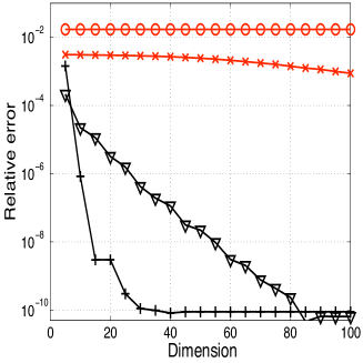
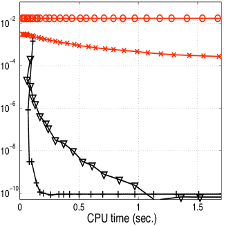
(a) (b)

Fig. 16: Convergence of the time-stepping algorithm in dependence of (a) dimension $K$ of Krylov subspaces and (b) CPU time needed to determine the profile variation $u$ for one time-step. The example used is the 1d dewetting problem (section 5.1) with parameters as in Fig. 3(b). Results are given for two sets of computational parameters – set 1 has time-step $\tau_{1}/\tau_{m}=0.08$, initial profile $h_{1}$ at time $t_{1}=10\tau_{m}$; and set 2 has time-step $\tau_{2}=100\tau_{m}$, initial profile $h_{2}$ at time $t_{2}=2\cdot 10^{3}\tau_{m}\simeq\tau_{\lambda}$. Convergence is shown for the simple Arnoldi method (symbols “$\color[rgb]{1,0,0}{\times}$” for set 1, “o” for set 2), and the Cayley-Arnoldi method (symbols “$\nabla$” for set 1, “$+$” for set 2).

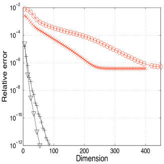
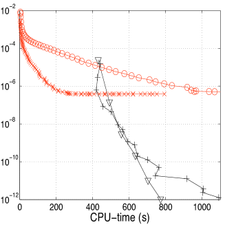
(a) (b)

Fig. 17: Convergence of the time-stepping algorithm in dependence of (a) dimension $K$ of Krylov subspaces and (b) CPU time needed to determine the profile variation $u$ for one time-step. The example used is the 2d dewetting problem (section 5.2) with parameters as in Fig. 9(b). Results are given for two sets of computational parameters – set 1 has time-step $\tau_{1}=0.05\tau_{m}\simeq\tau_{\lambda}$, initial profile $h_{0}$ at time $t=22\tau_{m}$; and set 2 has time-step $\tau_{2}=0.15\tau_{m}\simeq\tau_{\lambda}$, and $h_{0}$ as set 1. Convergence is shown for the simple Arnoldi method (symbols “$\color[rgb]{1,0,0}{\times}$” for set 1, “o” for set 2), and the Cayley-Arnoldi method (symbols “$\nabla$” for set 1, “$+$” for set 2).

Appendix B Comparison to classical algorithm

$\mathbf{J}$ using the ILU factorization. As the complexity of this task is $O(N^{3/2})$ the CPU cost is a more important issue than in other schemes.

If one implemented a classical implicit time integrator one would need to solve a linear system involving the matrix $\mathbf{J}$. For instance, a backward Euler scheme leads to the system $(\mathbf{I}+\mathbf{J}\tau)u=b\tau$, where $b$ is a known vector. A typical choice for the latter is the use of an iterative Krylov method as, e.g., the GEMRES method which is a good candidate for asymmetric matrices. The efficiency of this method does strongly depend on the knowledge of an effective preconditioner. Without preconditioner, the inversion for a simple semi-implicit scheme (backward Euler) converges very slowly and almost fails to obtain the wanted tolerance. Since no general preconditioner exists for the asymmetric matrix $\mathbf{J}$, its ILU factorization appears to be the only systematic way to construct an effective preconditioner. Therefore, a clear analogy exists between the exponential scheme and a semi-implicit scheme. On the one hand the Arnoldi algorithm to compute $G(\mathbf{J}\tau)$ is equivalent to the use of an iterative method without preconditioner to solve the linear system in an implicit scheme. On the other hand, the Cayley-Arnoldi algorithm to compute $G(\mathbf{J}\tau)$ is equivalent to an iterative method with $LU$ preconditioner to solve the linear system in an implicit scheme. Judging the complexity of the algorithm, a classical implicit and an exponential propagation algorithm are roughly equivalent schemes at the same order. However, exponential schemes seem to have two advantages:

• The $G$ and $\exp$ functions have a better leftmost spectrum filtering property than rational functions.

• Krylov techniques converge faster when employed for the evaluation of $G(\mathbf{J}\tau)b$ and $\exp(\mathbf{J}\tau)$ than when employed for the solution of a linear system [39].

Furthermore, the Cayley-Arnoldi exponential propagation method used has the ability to give an estimate of the leading eigenvalues what the implicit method is not able to do. This information allows for an adaptive time-step that constitutes a major advantage when studying dynamics characterized by several time scales. In addition, it is an important information that allows one to perform non-standard stability analysis as, e.g., employed by Münch [59] to detect a fingering instability in dewetting.

Although the shift Cayley-transform is a standard method to find the rightmost eigenvalues of a operator [101] its application in a continuation algorithm is less common. However, when solving a linear system within the Newton algorithm one faces similar problems as discussed for time-stepping. Thus, an effective solution method requires the use of the $LU$ preconditioner. However, our algorithm does not use the ILU factorization for a direct inversion, but rather to find the rightmost eigenvalues. The advantage of this approach is the ability to determine the tangent direction even close to a saddle-node bifurcation. Furthermore, at a bifurcation point, the directions of (different) bifurcating branches can be found as set of tangent directions.

We emphasize that the numerical difficulties encountered in the time-stepping and the continuation task are both resolved using the Cayley transform. This reminds Ref. [99] where it is pointed out that algorithms overcoming the numerical difficulties encountered during a time-stepping scheme can be adapted to perform the bifurcation tasks. The developed algorithms overcome two main problems: (i) the operator has no ’simple’ relevant linear part (different spatial scaling), and (ii) the “very bad” conditioning of the Jacobian. With the current computers, the Cayley-Arnoldi method is the most efficient method for a moderate system size of $N=O(10^{5})$. In consequence, the scheme is difficult to adapt for three-dimensional PDEs.

Acknowledgments

We acknowledge support by the European Union via the FP7 Marie Curie scheme [Grant PITN-GA-2008-214919 (MULTIFLOW)] and by the Deutsche Forschungsgemeinschaft under grant SFB 486, project B13. We also thank the Max-Planck-Institut für Physik komplexer Systeme in Dresden (Germany) that hosted us during the early stage of the project. Finally, P.B. is grateful to L. S.  Tuckerman for fruitful discussions.

References

- [1] D. Bandyopadhyay, R. Gulabani, and A. Sharma, Stability and dynamics of bilayers, Ind. Eng. Chem. Res., 44 (2005), pp. 1259–1272.
- [2] D. Bandyopadhyay, A. Sharma, U. Thiele, and P. D. S. Reddy, Electric field induced interfacial instabilities and morphologies of thin viscous and elastic bilayers, Langmuir, 25 (2009), pp. 9108–9118.
- [3] J. Becker, G. Grün, R. Seemann, H. Mantz, K. Jacobs, K. R. Mecke, and R. Blossey, Complex dewetting scenarios captured by thin-film models, Nat. Mater., 2 (2003), pp. 59–63.
- [4] P. Beltrame, P. Hänggi and U. Thiele, Depinning of three-dimensional drops from wettability defects, Europhys. Lett., 86 (2009), p. 24006.
- [5] M. Ben Amar, L. Cummings, and Y. Pomeau, Singular points of a moving contact line, C R Acad. Sci. Ser. IIB, 329 (2001), pp. 277–282.
- [6] A. L. Bertozzi and M. P. Brenner, Linear stability and transient growth in driven contact lines, Phys. Fluids, 9 (1997), pp. 530–539.
- [7] A. L. Bertozzi, G. Grün, and T. P. Witelski, Dewetting films: Bifurcations and concentrations, Nonlinearity, 14 (2001), pp. 1569–1592.
- [8] A. L. Bertozzi, A. Münch, X. Fanton, and A. M. Cazabat, Contact line stability and ”undercompressive shocks” in driven thin film flow, Phys. Rev. Lett., 81 (1998), pp. 5169–5173.
- [9] A. L. Bertozzi, A. Münch, and M. Shearer, Undercompressive shocks in thin film flows, Physica D, 134 (1999), pp. 431–464.
- [10] M. Bestehorn and K. Neuffer, Surface patterns of laterally extended thin liquid films in three dimensions, Phys. Rev. Lett., 87 (2001), p. 046101.
- [11] M. Bestehorn, A. Pototsky, and U. Thiele, 3D large scale Marangoni convection in liquid films, Eur. Phys. J. B, 33 (2003), pp. 457–467.
- [12] D. Bonn, J. Eggers, J. Indekeu, J. Meunier, and E. Rolley, Wetting and spreading, Rev. Mod. Phys., 81 (2009), pp. 739–805.
- [13] H. S. Brown, I. G. Kevrekidis, A. Oron, and P. Rosenau, Bifurcations and pattern-formation in the regularized Kuramoto-Sivashinsky equation, Phys. Lett. A, 163 (1992), pp. 299–308.
- [14] J. M. Burgess, A. Juel, W. D. McCormick, J. B. Swift, and H. L. Swinney, Suppression of dripping from a ceiling, Phys. Rev. Lett., 86 (2001), pp. 1203–1206.
- [15] E. Buzano and M. Golubitsky, Bifurcation on the Hexagonal Lattice and the Planar Benard Problem, Phil. Trans. R. Soc. Lond. A, 308 (1983), pp. 617–667.
- [16] J. W. Cahn and J. E. Hilliard, Free energy of a nonuniform system. 1. Interfacual free energy, J. Chem. Phys., 28 (1958), pp. 258–267.
- [17] A. M. Cazabat, F. Heslot, S. M. Troian, and P. Carles, Fingering instability of thin spreading films driven by temperature gradients, Nature, 346 (1990), pp. 824–826.
- [18] L. Chen, L. Zhuang, P. Deshpande, and S. Chou, Novel polymer patterns formed by lithographically induced self-assembly (LISA), Langmuir, 21 (2005), pp. 818–821.
- [19] J. Conway, The orbifold notation for surface groups, in Groups, Combinatorics and Geometry, M. W. Liebeck and J. S. (eds.), eds., Proceedings of the L.M.S. Durham Symposium,, Durham, UK, July 5Ð15 1992.
- [20] B. P. Cook, A. L. Bertozzi, and A. E. Hosoi, Shock solutions for particle-laden thin films, SIAM J. Appl. Math., 68 (2008), pp. 760–783.
- [21] J. D. Crawford and E. Knobloch, Symmetry and symmetry-breaking bifurcations in fluid-dynamics, Ann. Rev. Fluid Mech., 23 (1991), pp. 341–387.
- [22] M. C. Cross and P. C. Hohenberg, Pattern formation out of equilibrium, Rev. Mod. Phys., 65 (1993), pp. 851–1112.
- [23] Z. Dagan and L. M. Pismen, Marangoni waves induced by a multistable chemical reaction on thin liquid films., J. Colloid Interface Sci., 99 (1984), pp. 215–225.
- [24] P.-G. de Gennes, Wetting: Statics and dynamics, Rev. Mod. Phys., 57 (1985), pp. 827–863.
- [25] R. J. Deissler and A. Oron, Stable localized patterns in thin liquid films, Phys. Rev. Lett., 68 (1992), pp. 2948–2951.
- [26] B. V. Derjaguin, N. V. Churaev, and V. M. Muller, Surface Forces, Consultants Bureau, New York, 1987.
- [27] J. A. Diez and L. Kondic, Computing three-dimensional thin film flows including contact lines, J. Comput. Phys., 183 (2002), pp. 274–306.
- [28] E. J. Doedel, A. R. Champneys, T. F. Fairgrieve, Y. A. Kuznetsov, B. Sandstede, and X. J. Wang, AUTO97: Continuation and bifurcation software for ordinary differential equations, Concordia University, Montreal, 2000.
- [29] M. H. Eres, L. W. Schwartz, and R. V. Roy, Fingering phenomena for driven coating films, Phys. Fluids, 12 (2000), pp. 1278–1295.
- [30] M. Fermigier, L. Limat, J. E. Wesfreid, P. Boudinet, and C. Quilliet, 2-dimensional patterns in Rayleigh-Taylor instability of a thin-layer, J. Fluid Mech., 236 (1992), pp. 349–383.
- [31] R. A. Friesner, L. S. Tuckerman, B. C. Dornblaser, and T. V. Russo, A method for exponential propagation of large systems of stiff nonlinear differential equations, J. Sci. Comp., 4 (1989), pp. 327–354.
- [32] S. Gasner, P. Blomgren, and A. Palacios, Noise-induced intermittency in cellular pattern-forming systems, Int. J. Bif. Chaos, 17 (2007), pp. 2765–2779.
- [33] K. B. Glaser and T. P. Witelski, Coarsening dynamics of dewetting films, Phys. Rev. E, 67 (2003), p. 016302.
- [34] A. A. Golovin, A. A. Nepomnyashchy, S. H. Davis, and M. A. Zaks, Convective Cahn-Hilliard models: From coarsening to roughening, Phys. Rev. Lett., 86 (2001), pp. 1550–1553.
- [35] G. Grün, On the convergence of entropy consistent schemes for lubrication type equations in multiple space dimensions, Math. Comput., 72 (2003), pp. 1251–79.
- [36] G. Grün and M. Rumpf, Simulation of singularities and instabilities arising in thin film flow, Euro. Jnl of Applied Mathematics, 12 (2001), pp. 293–320.
- [37] D. Ho, Tchebychev acceleration technique for large scale nonsymmetric matrices, Numer. Math., 56 (1990), pp. 721–734.
- [38] M. Hochbruck and C. Lubich, On krylov subspace approximations to the matrix exponential operator, SIAM J. Numer. Anal., 34 (1997), pp. 1552–1574.
- [39] M. Hochbruck, C. Lubich, and H. Selhofer, Exponential integrators for large systems of differential equations, SIAM J. Sci. Comp., 19 (1998), pp. 1552–1574.
- [40] J. N. Israelachvili, Intermolecular and Surface Forces, Academic Press, London, 1992.
- [41] O. E. Jensen and J. B. Grotberg, Insoluble surfactant spreading on a thin viscous film: Shock evolution and film rupture, J. Fluid Mech., 240 (1992), pp. 259–288.
- [42] K. John, M. Bär, and U. Thiele, Self-propelled running droplets on solid substrates driven by chemical reactions, Eur. Phys. J. E, 18 (2005), pp. 183–199.
- [43] K. John, P. Hänggi, and U. Thiele, Ratchet-driven fluid transport in bounded two-layer films of immiscible liquids, Soft Matter, 4 (2008), pp. 1183–1195.
- [44] S. Kalliadasis, Nonlinear instability of a contact line driven by gravity, J. Fluid Mech., 413 (2000), pp. 355–378.
- [45] S. Kalliadasis and U. Thiele, eds., Thin Films of Soft Matter, Springer, Wien / New York, 2007. CISM 490.
- [46] D. E. Kataoka and S. M. Troian, A theoretical study of instabilities at the advancing front of thermally driven coating films, J. Colloid Interface Sci., 192 (1997), pp. 350–362.
- [47] I. G. Kevrekidis, B. Nicolaenko, and J. C. Scovel, Back in the saddle again - a computer-assisted study of the Kuramoto-Sivashinsky equation, SIAM J. Appl. Math., 50 (1990), pp. 760–790.
- [48] R. Khanna, A. Sharma, and G. Reiter, The ABC of pattern evolution in self-destruction of thin polymer films, EPJdirect, E2 (2000), pp. 1–9.
- [49] V. Lapuerta, F. J. Mancebo, and J. M. Vega, Control of Rayleigh-Taylor instability by vertical vibration in large aspect ratio containers, Phys. Rev. E, 64 (2001), p. 016318.
- [50] N. Le Grand, A. Daerr, and L. Limat, Shape and motion of drops sliding down an inclined plane, J. Fluid Mech., 541 (2005), pp. 293–315.
- [51] J. Liesen and P. Tichý, Convergence analysis of Krylov subspace methods, GAMM Mitt. Ges. Angew. Math. Mech., 27 (2004), pp. 153–173.
- [52] Z. Lin, T. Kerle, S. M. Baker, D. A. Hoagland, E. Schäffer, U. Steiner, and T. P. Russell, Electric field induced instabilities at liquid/liquid interfaces, J. Chem. Phys., 114 (2001), pp. 2377–2381.
- [53] T. A. Manteuffel, The Tchebychev iteration for nonsymmetric linear systems, Numer. Math., 28 (1977), pp. 307–327.
- [54] O. K. Matar and R. V. Craster, Models for Marangoni drying, Phys. Fluids, 13 (2001), pp. 1869–1883.
- [55] K. Meerbergen and D. Roose, Matrix transformations for computing rightmost eigenvalues of large sparse non-symmetric eigenvalue problems, IMA J. Numer. Anal., 16 (1996), pp. 297–346.
- [56] D. Merkt, A. Pototsky, M. Bestehorn, and U. Thiele, Long-wave theory of bounded two-layer films with a free liquid-liquid interface: Short- and long-time evolution, Phys. Fluids, 17 (2005), p. 064104.
- [57] V. S. Mitlin, Dewetting of solid surface: Analogy with spinodal decomposition, J. Colloid Interface Sci., 156 (1993), pp. 491–497.
- [58] A. Münch, Pinch-off transition in Marangoni-driven thin films, Phys. Rev. Lett., 91 (2003), p. 016105.
- [59] , Dewetting rates of thin liquid films, J. Phys.: Condens. Matter, 17 (2005), pp. S309–S318.
- [60] A. Oron, Nonlinear dynamics of three-dimensional long-wave Marangoni instability in thin liquid films, Phys. Fluids, 12 (2000), pp. 1633–1645.
- [61] , Three-dimensional nonlinear dynamics of thin liquid films, Phys. Rev. Lett., 85 (2000), pp. 2108–2111.
- [62] A. Oron, S. H. Davis, and S. G. Bankoff, Long-scale evolution of thin liquid films, Rev. Mod. Phys., 69 (1997), pp. 931–980.
- [63] A. Oron and P. Rosenau, Formation of patterns induced by thermocapillarity and gravity, J. Physique II France, 2 (1992), pp. 131–146.
- [64] , On a nonlinear thermocapillary effect in thin liquid layers, J. Fluid Mech., 273 (1994), pp. 361–374.
- [65] A. Pereira, P. M. J. Trevelyan, U. Thiele, and S. Kalliadasis, Dynamics of a horizontal thin liquid film in the presence of reactive surfactants, Phys. Fluids, 19 (2007), p. 112102.
- [66] T. Podgorski, J.-M. Flesselles, and L. Limat, Corners, cusps, and pearls in running drops, Phys. Rev. Lett., 87 (2001), p. 036102.
- [67] A. Pototsky, M. Bestehorn, D. Merkt, and U. Thiele, Alternative pathways of dewetting for a thin liquid two-layer film, Phys. Rev. E, 70 (2004), p. 025201(R).
- [68] , Morphology changes in the evolution of liquid two-layer films, J. Chem. Phys., 122 (2005), p. 224711.
- [69] A. Pototsky, M. Bestehorn, D. Merkt, and U. Thiele, 3d surface patterns in liquid two-layer films, Europhys. Lett., 74 (2006), pp. 665–671.
- [70] G. Reiter, Dewetting of thin polymer films, Phys. Rev. Lett., 68 (1992), pp. 75–78.
- [71] G. Reiter and A. Sharma, Auto-optimization of dewetting rates by rim instabilities in slipping polymer films, Phys. Rev. Lett., 87 (2001), p. 166103.
- [72] E. Ruckenstein and R. K. Jain, Spontaneous rupture of thin liquid films, J. Chem. Soc. Faraday Trans. II, 70 (1974), pp. 132–147.
- [73] Y. Saad, Analysis of some krylov subspace approximations to the matrix exponential operator, SIAM J. Numer. Anal., 29 (1992), pp. 209–228.
- [74] M. Sadkane, A block Arnoldi-Chebyshev method for computing the leading eigenpairs of large sparse unsymmetric matrices, Numer. Math., 64 (1993), pp. 181–193.
- [75] R. Seemann, S. Herminghaus, C. Neto, S. Schlagowski, D. Podzimek, R. Konrad, H. Mantz, and K. Jacobs, Dynamics and structure formation in thin polymer melt films, J. Phys.-Condes. Matter, 17 (2005), pp. S267–S290.
- [76] R. Seydel, Practical Bifurcation and Stability Analysis, Springer-Verlag, New York, 1994.
- [77] A. Sharma, Relationship of thin film stability and morphology to macroscopic parameters of wetting in the apolar and polar systems, Langmuir, 9 (1993), pp. 861–869.
- [78] A. Sharma and R. Khanna, Pattern formation in unstable thin liquid films, Phys. Rev. Lett., 81 (1998), pp. 3463–3466.
- [79] A. Sharma and G. Reiter, Instability of thin polymer films on coated substrates: Rupture, dewetting and drop formation, J. Colloid Interface Sci., 178 (1996), pp. 383–399.
- [80] J. H. Snoeijer, E. Rio, N. Le Grand, and L. Limat, Self-similar flow and contact line geometry at the rear of cornered drops, Phys. Fluids, 17 (2005), p. 072101.
- [81] M. A. Spaid and G. M. Homsy, Stability of Newtonian and viscoelastic dynamic contact lines, Phys. Fluids, 8 (1996), pp. 460–478.
- [82] J. Sur, A. L. Bertozzi, and R. P. Behringer, Reverse undercompressive shock structures in driven thin film flow, Phys. Rev. Lett., 90 (2003), p. 126105.
- [83] U. Thiele, Open questions and promising new fields in dewetting, Eur. Phys. J. E, 12 (2003), pp. 409–416.
- [84] , Structure formation in thin liquid films, in Thin films of Soft Matter, S. Kalliadasis and U. Thiele, eds., Wien, 2007, Springer, pp. 25–93.
- [85] U. Thiele, Thin film evolution equations from (evaporating) dewetting liquid layers to epitaxial growth, J. Phys.-Cond. Mat., 22 (2010), p. 084019. (at press).
- [86] U. Thiele, L. Brusch, M. Bestehorn, and M. Bär, Modelling thin-film dewetting on structured substrates and templates: Bifurcation analysis and numerical simulations, Eur. Phys. J. E, 11 (2003), pp. 255–271.
- [87] U. Thiele, B. Goyeau, and M. G. Velarde, Film flow on a porous substrate, Phys. Fluids, 21 (2009), p. 014103.
- [88] U. Thiele, K. John, and M. Bär, Dynamical model for chemically driven running droplets, Phys. Rev. Lett., 93 (2004), p. 027802.
- [89] U. Thiele and E. Knobloch, Front and back instability of a liquid film on a slightly inclined plate, Phys. Fluids, 15 (2003), pp. 892–907.
- [90] U. Thiele and E. Knobloch, Thin liquid films on a slightly inclined heated plate, Physica D, 190 (2004), pp. 213–248.
- [91] , Driven drops on heterogeneous substrates: Onset of sliding motion, Phys. Rev. Lett., 97 (2006), p. 204501.
- [92] , On the depinning of a driven drop on a heterogeneous substrate, New J. Phys., 8 (2006), pp. 313, 1–37.
- [93] U. Thiele, I. Vancea, A. J. Archer, M. J. Robbins, L. Frastia, A. Stannard, E. Pauliac-Vaujour, C. P. Martin, M. O. Blunt, and P. J. Moriarty, Modelling approaches to the dewetting of evaporating thin films of nanoparticle suspensions, J. Phys.-Cond. Mat., 21 (2009), p. 264016.
- [94] U. Thiele, J. M. Vega, and E. Knobloch, Long-wave Marangoni instability with vibration, J. Fluid Mech., 546 (2006), pp. 61–87.
- [95] U. Thiele, M. G. Velarde, and K. Neuffer, Dewetting: Film rupture by nucleation in the spinodal regime, Phys. Rev. Lett., 87 (2001), p. 016104.
- [96] U. Thiele, M. G. Velarde, K. Neuffer, M. Bestehorn, and Y. Pomeau, Sliding drops in the diffuse interface model coupled to hydrodynamics, Phys. Rev. E, 64 (2001), p. 061601.
- [97] U. Thiele, M. G. Velarde, K. Neuffer, and Y. Pomeau, Film rupture in the diffuse interface model coupled to hydrodynamics, Phys. Rev. E, 64 (2001), p. 031602.
- [98] M. Tokman, Efficient integration of large stiff systems of odes with exponential propagation (epi) methods, J. Comput. Phys., 213 (2006), pp. 748–776.
- [99] L. S. Tuckerman and D. Barkley, Bifurcation analysis for timesteppers, in Numerical Methods for Bifurcation Problems and Large-Scale Dynamical, L. Doedel, E. andTuckerman, ed., vol. 119 of IMA Volumes in Mathematics and its Applications, New-York, 2000, Springer, pp. 466–543.
- [100] R. Verma, A. Sharma, K. Kargupta, and J. Bhaumik, Electric field induced instability and pattern formation in thin liquid films, Langmuir, 21 (2005), pp. 3710–3721.
- [101] P. Wheeler and D. Barkley, Computation of spiral spectra, SIAM J. Applied Dynamical Systems, 5 (2006), pp. 157–177.
- [102] T. Witelski and M. Bowen, Adi schemes for higher-order nonlinear diffusion equations, Applied Numerical Mathematics, 45 (2003), p. 331Ð351.
- [103] L. Zhornitskaya and A. L. Bertozzi, Positivity-preserving numerical schemes for lubrication-type equations, SIAM J. Numer. Anal., 37 (2000), pp. 523–555.