Atomic-ensemble-based quantum memory for sideband modulations

Abstract

Interaction of a control and a signal field with an ensemble of three-level atoms allows direct mapping of the quantum state of the signal field into long lived coherences of an atomic ground state. For a vapor of cesium atoms, using Electromagnetically Induced Transparency (EIT) and Zeeman coherences, we compare the case where a tunable single-sideband is stored independently of the other one to the case where the two symmetrical sidebands are stored using the same transparency window. We study the conditions in which simultaneous storage of two non-commuting variables carried by light and subsequent read-out is possible. We show that excess noise associated with spontaneous emission and spin relaxation is small, and we evaluate the quantum performance of our memory by measuring the signal transfer coefficient T and the conditional variance V and using the T-V criterion as a state independent benchmark.

I Introduction

Quantum information technology is a fast developing field, which aims to exploit new ways for information processing and communication with no analogue in classical information science. This paradigm leads in particular towards absolutely secure communications and computing powers beyond the capacities of any classical computer. Quantum communications, in particular scalable networks, as well as quantum computation rely critically on memory registers and considerable interests are currently dedicated to this quest zoller ; kimble .

Developing registers for quantum variables requires however completely different concepts than for classical data. In such systems, photonic quantum data must be linearly and reversibly converted into long-lived matter states. Atomic ensembles are good candidates for such memory since quantum states of light can be stored in long-lived atomic spin states by means of light-matter interaction and retrieved on demand. Starting around the year 2000, several protocols have been proposed for light-matter interfacing. Different configurations have been studied, including Raman-type configuration Polzik1 ; DLCZ ; Dantan1 , resonant electromagnetically induced transparency (EIT) scheme Lukin1 ; Lukin2 ; Dantan2 or quantum non demolition (QND) interaction using a X-type transition Polzik2 . Rephasing photon echo or spin echo interactions for storage and read-out of the quantum signal have also been studied Moiseev ; Kraus ; Sangouard .

Considerable experimental works have been performed in the single photon regime, including probabilistic protocols in Raman configuration james ; julien ; james2 ; Pan ; Vuletic or storage and read-out of single photons using the EIT scheme Lukin3 ; Kuzmich . Recent papers present notable advances with reversible mapping of single-photon entanglement Choi and enhanced memory time Zhao . For future quantum communications, continuous variables may offer improved data transmission rates Grangier , and, in this paper, we will focus on this regime. Storage of non-commuting quantum variables of a light pulse has been demonstrated in 2004 Polzik3 , however without the possibility of read-out. Significantly, very recent results demonstrated storage and retrieval of a squeezed light pulse, or of faint coherent state with quantum performances Kozuma ; Lvovsky ; Cviklinski .

Presently, while advances have been achieved in the direction of a deterministic quantum memory, it is interesting to investigate a variety of different systems allowing more flexibility. In this paper, we compare the potential of the EIT scheme when quantum sidebands are stored independently, to the case where two sidebands are stored in the same EIT window. In particular, we show that when single sidebands are stored on an adjustable frequency range, using the Zeeman coherence of the atoms, the optimal response of the medium for storage can be adapted to the frequency to be stored by changing the magnetic field, while keeping a narrow EIT window. If symmetrical sidebands are stored in separate atomic ensembles, this method should allow the storage of a variety of quantum signals. This opens the way to quantum storage and retrieval of quantum fluctuations with adjustable frequency.

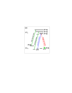
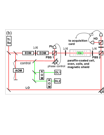
Figure 1: (a) Cesium atomic levels and transitions involved in the experiment. (b) Schematic diagram of the experimental setup. The Ti-sapphire laser generates a beam which is used as the control beam; a part of it is split off and frequency shifted by two electro-optic modulators (E.O.M.) to generate the signal beam . The two beams are recombined on a polarizing beamsplitter (PBS1) and sent into the cell together with the pumping and repumping beams produced by diode lasers DL1 and DL2, the frequencies of which are adjusted with acousto-optic modulators (A.O.M.). The beam going out of the cell is mixed with a local oscillator (with the same frequency as the control beam) on polarizing beamsplitter PBS2 and sent to a homodyne detection (H.D.)

II EIT-based quantum memory

We consider a large ensemble of N three-level atoms in a $\Lambda$ configuration, with two ground states and one excited state. The storage protocol relies on two light fields, the control field and the signal field, that interact with the atoms, with frequencies close to resonance with the two atomic transitions. For optimal efficiency, the two-photon resonance must be fulfilled. The control field is a strong, classical field that makes the medium transparent by way of EIT for the signal field to be stored Harris . The signal field is a very weak coherent field. If the control field is strong enough, the atomic medium becomes transparent for the signal field, and the refractive index acquires a very high slope as a function of frequency in the vicinity of the one-photon resonance. Thus the group velocity for the signal field is strongly reduced Hau1 ; Hau2 ; Phillips .

When the signal pulse is entirely inside the atomic medium and after a write time, which is on the order of the characteristic interaction time between atoms and fields, the control field can be switched off. The two quadratures of the signal are then stored in two components of the ground state coherence. For read-out, the control field is turned on again. The medium emits a weak pulse, similar to the original signal pulse, that goes out of the medium together with the control field.

Models developed in Refs Lukin1 ; Lukin2 ; Dantan2 predict that the classical mean values as well as the quantum variables of the field can be stored with a high efficiency as collective spin variables, and that the quantum variables can be retrieved in the outgoing pulse with a very good efficiency Dantan3 ; Sorensen . Taking into account all the noise sources, including the atomic noise generated by spontaneous emission and spin relaxation, a significant result of theoretical models Dantan2 ; Dantan3 ; Sorensen is the absence of excess noise in the process of storage and retrieval, provided the optical depth of the medium is large enough.

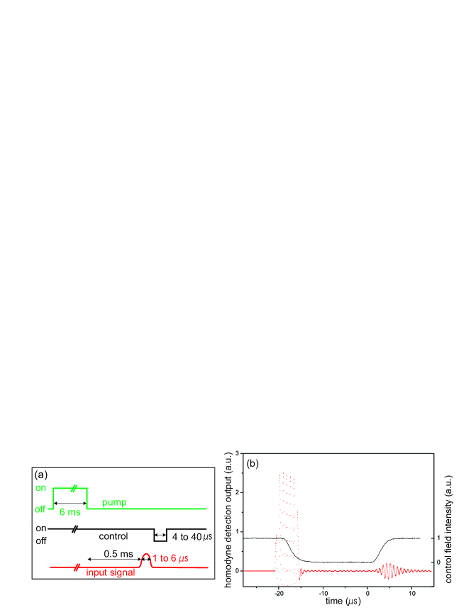
Figure 2: (a) Detail of the experimental sequence. (b) Temporal profile of the control field during the writing, storage and reading stage (solid line), together with the homodyne detection output current (dots) for a macroscopic 4 $\mu$W input pulse, in arbitrary units.

III Experimental scheme

The level configuration is shown in Fig. 1(a). It involves the transition $6S_{1/2},F=3$ to $6P_{3/2},F^{\prime}=2$ of the Cesium D₂ line. More specifically, the control beam is $\sigma^{+}$ polarized and resonant with the $m_{F}=1$ to $m_{F^{\prime}}=2$ transition while the signal field is $\sigma^{-}$ polarized and resonant with the $m_{F}=3$ to $m_{F^{\prime}}=2$ transition (Fig. 1(a)). In order to fulfill the two-photon resonance condition, the detuning $\Omega$ between the control and signal beams is set to be equal to the Zeeman shift $2\Omega_{L}$ between the $m_{F}=1$ and $m_{F}=3$ sublevels of the ground state

$$\Omega=2\Omega_{L}=2\mu_{B}gH$$ (1)

where $g$ is the Landé factor, $\mu_{B}$ the Bohr magneton and $H$ is the magnetic field. By tuning the magnetic field, one can optimize the memory response for a given frequency, allowing a widely tunable frequency range for the signal to be stored.

The experimental set-up is sketched on Fig. 1(b). The Cesium vapor is contained in a 3 cm long cell with a paraffin coating that suppresses ground state decoherence caused by collisions with the walls. The cell is heated to temperatures ranging from 30^oC to 40^oC, yielding optical depths from 6 to 18 on the signal transition. It is placed in a longitudinal magnetic field adjustable between 0 and 2 Gauss produced by symmetrical sets of coils and in a magnetic shield made of three layers of $\mu$metal. Residual magnetic fields are smaller than 0.2 mG, and the homogeneity of the applied magnetic field over the cell volume, measured by magneto-optical resonance, is better than 1:700. The atoms are optically pumped from the F=4 to the F=3 ground state and into the $m_{F}=3$ sublevel of the F=3 ground state with diode lasers, as shown in Fig. 1(b). The control and signal beams are produced by a single-mode, Ti-Sapphire laser, with a linewidth of 100 kHz, stabilized on a saturated transition absorption. The control beam fluctuations are at the shot-noise limit for frequencies above 1 MHz.

The signal beam is produced by splitting off a part of the control beam and generating a single sideband shifted from the initial frequency by using a set of two electro-optic modulators separated by wave plates and polarizers, as described in Cusack . The second sideband is suppressed by 20 dB. The single sideband is a very weak coherent field, with a power on the order of a nanowatt, with an adjustable frequency detuning $\Omega$ and with a polarization perpendicular to that of the carrier. The carrier is filtered out by reflection on a polarizing beam splitter (PBS1 in Fig. 1(b)), the reflected beam being used to lock the signal to control relative phase. The control field from the Ti-Sapphire laser, with a power of 10 to 140 mW, can be turned on and off with an acousto-optic modulator. It has a vertical polarization, and it is mixed with the horizontally polarized weak signal beam on the same polarizing beamsplitter. The beam is sent into the cell after passing through a quarter-wave plate, which produces the $\sigma^{+}$ and $\sigma^{-}$ polarizations.

IV Detection

The light going out of the cell is mixed with a local oscillator and analyzed using a homodyne detection, after eliminating the control beam by means of a polarizing beamsplitter (PBS2 in Fig. 1(b)). The local oscillator is obtained from the same Ti-Sapphire laser as the control and signal beams and has the same frequency as the control beam. Its phase is locked to the one of the control beam.

The photocurrent difference obtained after the homodyne detection yields the amplitude modulation operator $\hat{X}(\Omega)$:

$$\hat{i}=\hat{X}(\Omega)=(\hat{X}_{\Omega}+\hat{X}_{-\Omega})\cos\Omega t+(\hat{Y}_{\Omega}-\hat{Y}_{-\Omega})\sin\Omega t$$ (2)

which is expressed as a combination of the quadrature operators of the two sidebands, $\hat{X}_{\pm\Omega}$ and $\hat{Y}_{\pm\Omega}$. Since the two operators $\hat{X}_{\Omega}+\hat{X}_{-\Omega}$ and $\hat{Y}_{\Omega}-\hat{Y}_{-\Omega}$ commute, one can measure them at the same time on the sine and cosine components. However, the modulated signal field has only one sideband, so the components $\hat{X}_{-\Omega}$ and $\hat{Y}_{-\Omega}$ at $-\Omega$ are empty, corresponding to one unit of shot noise in the opposite sideband, which is an intrinsic feature of homodyne detection in this case.

In the experimental timing shown in Fig. 2(a), the atoms are first pumped into the $m_{F}=3$ sublevel of the $6S_{1/2},F=3$ level, using a $\sigma_{+}$ pumping diode laser, with a power of 0.2 mW, in the presence of an additional diode laser repumping the atoms from the $6S_{1/2},F=4$ level to the $6S_{1/2},F=3$ level, with a power of 2 mW. The pumping stage lasts for 6 ms, after which more than 90$\%$ of the atoms are pumped into the $m_{F}=3$ sublevel, as shown in Fig. 1 (a). After a dark period of 0.5 ms for the pumping and repumping laser diodes, the signal pulse is sent into the cell for the writing procedure, the control field being on. The signal pulse can last for 1 to 6 $\mu$s. The control and signal fields are then switched off for 4 to 40 $\mu$s, and the control field alone is turned on again. Fig. 2(b) shows the beat signal of the light going out of the cell with the local oscillator. The first pulse corresponds to the signal field transmitted during the writing period, the second one to the field read out from the signal stored by the atoms.

The photocurrent difference from the homodyne detection is recorded at a rate of 50 Megasamples per second with a 14 bits acquisition card (National Instruments NI 5122). A Fourier transform is performed digitally by multiplying the signal with a sine or a cosine function of angular frequency $\Omega$ and integrating over a time $t_{m}=n2\pi/\Omega$, with $n$=2 to 4. This yields sets of measured values of the quadrature operators $\hat{X}_{\Omega}$ and $\hat{Y}_{\Omega}$ of the outgoing field. Averaging over 2000 realizations of the experiment gives direct access to the quantum mean values $<\hat{X}_{\Omega}>$ and $<\hat{Y}_{\Omega}>$ and variances $<(\Delta\hat{X}_{\Omega})^{2}>=<(\hat{X}_{\Omega})^{2}>-(<\hat{X}_{\Omega}>)^{2}$ and $<(\Delta\hat{Y}_{\Omega})^{2}>=<(\hat{Y}_{\Omega})^{2}>-(<\hat{Y}_{\Omega}>)^{2}$ of the signal field quadratures.

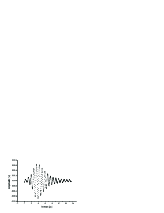
Figure 3: Typical temporal profile used for demodulation in order to enhance the measurement efficiency.

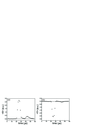
Figure 4: Time-dependent mean values of the amplitude (a) and phase (b) quadratures, measured from a typical 2000-sequence run (see text for details). T=36^oC, control field power = 9 mW, input pulse duration : 5 $\mu$s, input intensity : 0.1 nW.

In order to improve the efficiency of the measurement of the output signal, the temporal profile of the local oscillator must be adapted to the one of the signal Dantan3 . In an equivalent way, one can adapt the profile of the sine or cosine function used during demodulation. Figure 3 represents the optimal shape of the function used during the Fourier transform yielding the values of $\hat{X}$ and $\hat{Y}$. Using this profile instead of a usual sine function with a constant amplitude improves the measurement efficiency by a factor 3, because it avoids measuring the vacuum field outside the relevant time interval of the pulse. This improved profile is created by recording the signal going out of the memory in the case of a macroscopic signal (with a power of a few microwatts).

V Experimental results

Typical traces are shown in Fig. 4. The first peak corresponds to the transmitted part of signal field, the second part to the retrieved signal, for the in-phase ($X$) quadrature (curve (a)) and for the out-of-phase ($Y$) quadrature (curve (b)).

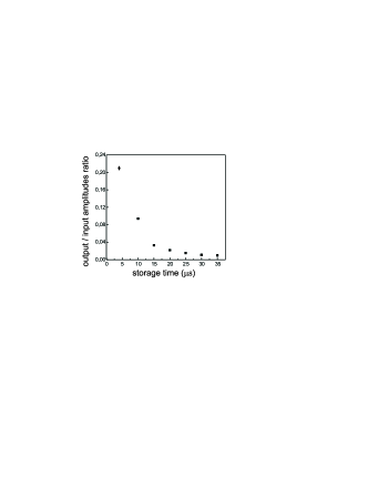
Figure 5: Ratio of the amplitudes of the input and output states, as a function of the storage time. T=40^oC. The points indicated by $\blacksquare$ $(\blacklozenge)$ correspond to a signal pulse duration of 6.4 $\mu\mathrm{s}$ (1.6 $\mu\mathrm{s}$) with a control field power of 10 mW (140 mW).

As far as the mean values are concerned, Fig. 4 shows that the experiment allows to store the two quadratures of a signal in the atomic ensemble and then to retrieve them. The retrieved signal is about 10$\%$ of the transmitted signal in amplitude. The storage efficiency as a function of the storage time is shown in Fig. 5. The storage efficiency decreases rapidly with the storage time, with a time constant $\tau_{m}\sim 10\,\mu$s, due to spin relaxation in the ground state, in particular because of stray magnetic fields and collisions. An efficiency of 21$\%$ is measured for a short storage time with a strong control field.

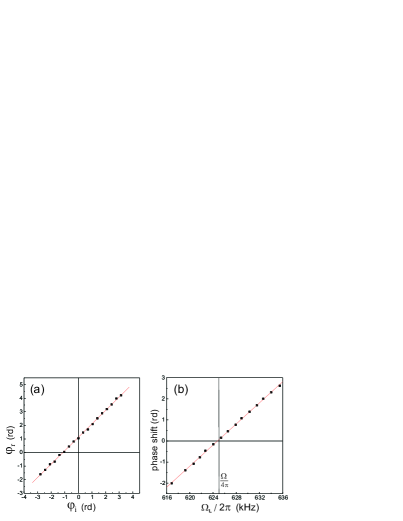
Figure 6: Dependence of the retrieved pulse phase, as a function of the input pulse phase with a constant Larmor frequency (a), and as a function of the Larmor frequency (b) (i.e : as a function of the two-photon detuning), with a fixed phase for the input phase. The storage time is 20 $\mu$s, and $\Omega/2\pi=$1.25 MHz.

In order to check the phase coherence of the process, we have performed a detailed study of the phase of the retrieved signal coherence . When the two photon transition resonance with the control field and the signal field is fulfilled, $\delta=2\Omega_{L}-\Omega=0$, the atomic coherence evolves during the storage time with a frequency which is equal to $\Omega$. When the control field is sent again into the atomic ensemble for read-out (with a phase that is still locked to the phase of the local oscillator), the outgoing field is expected to be emitted with the same phase relative to the control field as the one of the signal field. If the two-photon transition is slightly off resonance, the atomic coherence accumulates a phase difference during the storage time. This causes a phase shift of the retrieved signal as compared to the control field.

Figure 6(a) shows the measured dependence of the phase $\varphi_{r}$ of the retrieved pulse on the phase $\varphi_{i}$ of the initial pulse. Phase $\varphi_{r}$ shows a linear dependence on $\varphi_{i}$ with a unit slope, confirming the coherence of the process, while the non-zero value of $\varphi_{r}$ for $\varphi_{i}=0$ corresponds to a small two-photon detuning in the storage process. We show in figure 6(b) the measured phase shift of the retrieved signal as a function of $\delta$ by varying the magnetic field for a fixed storage time. The phase shift shows a linear dependence on the Larmor frequency, with a slope of 0.25 rd/kHz which is in very good agreement with the predicted dependence, given by $\varphi_{r}=(2\Omega_{L}-\Omega)\tau$, where $\tau$= 20 $\mu$s is the storage time. These measurements show the full phase coherence of the process.

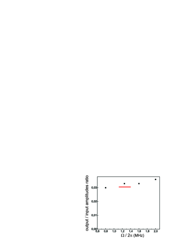
Figure 7: Ratio of the amplitudes of the input and output states, as a function of the modulation frequency $\Omega/2\pi$. The bar indicates the spectral width of the input pulse.

In this experiment we store a very weak coherent field that, as explained before, can be considered as a single modulation sideband of the control field. This allows more flexibility than storing two symmetrical sidebands in the same EIT window, especially for high frequency components. We have measured the efficiency of the process when the sideband frequency $\Omega$ is varied, as can be seen in Fig. 7. No significant variation with $\Omega$ is observed. This comes from the fact that the frequency of the signal to be stored can be matched to the position of the EIT window, without changing its width. The EIT window width can be kept below 1 MHz, as shown in Fig. 8(a).

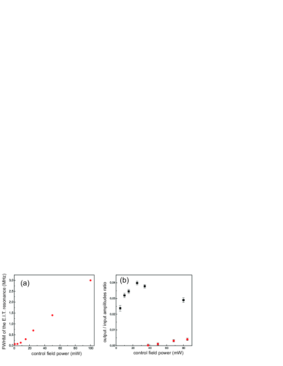
Figure 8: (a) Full width at half maximum of the EIT transparency window (MHz) as a function of the control field power (mW). The control and probe beams 1/$e^{2}$ radius is $7.2$ mm. (b) Ratio of the output and input states amplitudes, as a function of the control field power, for a single sideband of frequency 1.25 MHz (squares) and a dual sideband modulation of frequency 400 kHz. T= 50 ^o C . Pulse duration : 5 $\mu\mathrm{s}$. Storage time : 15 $\mu\mathrm{s}$.

The two sidebands of a field can also be stored at the same time if $2\Omega$ is smaller than the EIT linewidth. Figure 8(a) shows the EIT linewidth in our case as a function of the control field power. For a control field power $P_{c}\sim 40$ mW, the full width at half maximum of the EIT resonance is of the order of 1 MHz. We have measured the efficiency of the storage process for a signal field made of two sidebands at $\pm$400 kHz. The result is shown in Fig. 8(b). The efficiency is lower than in the single sideband case, which can be attributed to the large value of the time-bandwith product of the pulse to be stored.

VI Noise characteristics

A critical feature for a quantum memory is the noise characteristics of the outgoing signal. The noise curves shown in Fig. 9(a) correspond to the mean values shown in Fig. 4 and are obtained by calculating the variances from the same data set. Because of a small leak of the control field into the signal field channel, the raw data exhibit additional features due to the transients of the control field. Although it has been designed with a smooth shape, the latter contains Fourier components around $\Omega/2\pi=1.2$ MHz. To get rid of this spurious effect, we have used a subtraction procedure. The transients are measured independently after each sequence with no signal field and the corresponding data are subtracted point to point from the data taken with a signal field. The signal curves shown in Fig. 4 are obtained with this method. For the noise, this procedure is equivalent to a 50/50 beamsplitter on the analyzed beam and adds one unit of shot noise to the noise that would be measured without the subtraction, yielding the upper curve in Fig. 9(a) for the variance of the amplitude quadrature. The variance of the phase quadrature behaves in a similar way. The noise calculated from the raw data, without subtraction, corresponding to the lower curve in Fig. 9(a) exhibits a small amount of additional fluctuations when the control field is turned on for read-out. With the subtraction procedure, these fluctuations are suppressed, showing that they originate from a classical, reproducible spurious effect.

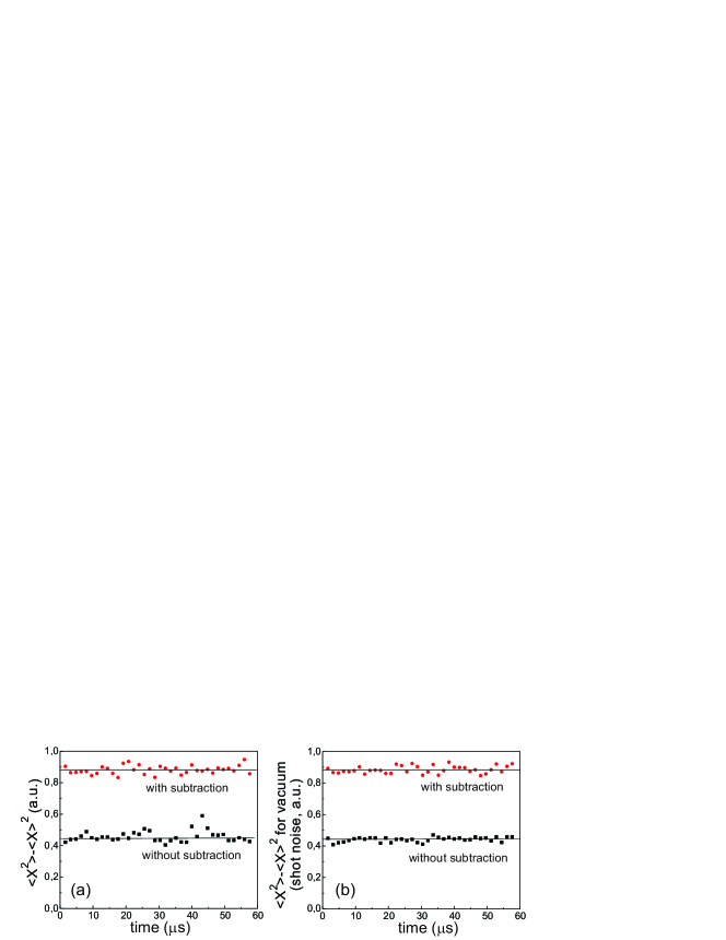
Figure 9: Variance of the amplitude quadrature for the signal (a) and for the vacuum (b). The units are arbitrary and are the same in (a) and (b) and for the mean values squared in Fig. 4.

The noise curves can be compared to the shot noise, which is obtained independently from the same procedure with no control field and no signal field in the input, without and with subtraction, as shown in Fig. 9(a). The recorded variances shown in Fig. 9(a) are found to be at the same level as shot noise (Fig. 9(b)), which indicates that the writing and reading processes add very little noise. From these measurements, excess noise can be evaluated to be zero with an uncertainty of less than 2$\%$. The noise curves of Fig. 9(a) correspond to moderate values of the control field power (10 mW). When the control field power is set to higher values, excess noise appears. Excess noise has been studied by other authors Lam ; Hetet . In our case, it originates from fluorescence and coherent emission due to the control beam Lvovsky and from spurious fluctuations from the turn on of the control field leaking into the signal channel, that cannot be eliminated with the subtraction procedure.

Following Ref. Hetet , we can evaluate the quantum performance of our storage device using criteria derived from the T-V characterization. This method was proposed in Ref. Roch to characterize quantum non demolition measurements or teleportation, and allows to obtain a state independent quantum benchmark. The conditional variance product $V$ of the signal field quadratures before and after storage is the geometrical mean value of the input-output conditional variances $V=\sqrt{V_{X}V_{Y}}$ of the two quadratures, with

$$V_{X}=V_{X}^{out}-\frac{|\langle\hat{X}^{in}\hat{X}^{out}\rangle|^{2}}{V_{X}^{in}}$$ (3)

$$V_{Y}=V_{Y}^{out}-\frac{|\langle\hat{Y}^{in}\hat{Y}^{out}\rangle|^{2}}{V_{Y}^{in}}$$ (4)

where $V_{X}^{in/out}$ ($V_{Y}^{in/out}$) is the variance of the normalized input/output field quadratures denoted $\hat{X}^{in/out}$ ($\hat{Y}^{in/out}$). The total signal transfer coefficient $T$ is the sum of the transfer coefficients for the two quadratures

$$T=T_{X}+T_{Y}$$ (5)

with

$$T_{X}=\frac{\mathcal{R}_{X}^{out}}{\mathcal{R}_{X}^{in}}\hskip 28.45274ptT_{Y}=\frac{\mathcal{R}_{Y}^{out}}{\mathcal{R}_{Y}^{in}}$$ (6)

where $\mathcal{R}_{X}^{in/out}$ ($\mathcal{R}_{Y}^{in/out}$) is the signal to noise ratio of input/output field for the $X$ ($Y$) quadrature

$$\mathcal{R}_{X}^{in/out}=\frac{4(\alpha_{X}^{in/out})^{2}}{V_{X}^{in/out}}\hskip 28.45274pt\mathcal{R}_{Y}^{in/out}=\frac{4(\alpha_{Y}^{in/out})^{2}}{V_{Y}^{in/out}}$$ (7)

where $\alpha_{X}^{in/out}$ ($\alpha_{Y}^{in/out}$) is the mean amplitude of the field $\hat{X}^{in/out}$ ($\hat{Y}^{in/out}$) quadrature .

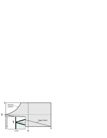
Figure 10: T-V diagram. Plot of the conditional variance product $V$ versus total signal transfer coefficient $T$. The upper curve shows the optimal performance of a classical memory. The linear loss curve corresponds to an unperfect memory register that introduces losses but no excess noise.

The experimental results shown in Fig. 4 and 9, with a storage amplitude efficiency of 10$\%$, correspond to $T=0.02$ and $V=0.99$, if one considers that the noise is equal to shot noise, and $V=1.01$ if the noise is 2$\%$ higher than shot noise. This case is represented by the bar represented in Fig. 10. A classical memory with the same $T$, represented by the upper curve in Fig. 10, yields $V=1.01$. So, in this case, the performances of our system are within the limit of the quantum domain. When the storage amplitude efficiency is 21$\%$, which is obtained with a smaller storage time and a higher control field, $T=0.08$, while the value of the conditional variance of a system with such a $T$ without excess noise is $V=0.96$ and the conditional variance for a classical memory is $V=1.04$. The excess noise in our experiment in that case is over 10$\%$, which corresponds to a performance well into the classical domain. With the experimental parameters used here, models Sorensen predict much higher efficiencies, of the order of 35$\%$ and no excess noise. The discrepancy can be attributed to the fact that the D2 line of Cesium is far from a simple $\Lambda$ scheme, and to decoherence effects in the lower levels.

VII Conclusion

In this paper, we have studied the storage and retrieval of the two non-commuting quadratures of a small coherent state in an atomic medium with very small excess noise. This coherent state, made of a single sideband of the control field, has been stored in the Zeeman coherence of the atoms. The optimal response frequency of the medium for storage can thus be adapted to the frequency to be stored by changing the magnetic field, keeping the EIT window rather narrow. Comparison with the storage of a modulation made of two symmetrical sidebands shows the latter is hampered by the finite bandwidth of the EIT window. Storing the two sidebands in two separate windows is thus a promising method for quantum memory with a widely adjustable frequency. For instance, in order to store squeezed fields at a given frequency $\Omega$, one has to store the two sidebands at $+\Omega$ and $-\Omega$. If $\Omega$ is large, this can be done in two separate ensembles, after separating the two sidebands using a Mach-Zehnder interferometer Leuchs or a cavity Ralph . After read-out, the two sidebands can be recombined. This procedure should lead to much higher efficiency than increasing the EIT window.

VIII Acknowledgements

This work was supported by the E. U. grants COVAQIAL and COMPAS, by the French ANR contract IRCOQ and by the Ile-de-France programme IFRAF. J.O. acknowledges support from the DGA and Dr. B. Desruelle.

References

- (1) P. Zoller et al., Eur. Phys. J. D 36, 203-228 (2005).
- (2) H.J. Kimble, Nature 453, 1023-1030 (2008).
- (3) A.E. Kozhekin, K. Mølmer, E.S. Polzik, Phys. Rev. A 62, 033809 (2000).
- (4) L.M. Duan, M.D. Lukin, J.I. Cirac and P. Zoller, Nature (London) 414, 413 (2001).
- (5) A. Dantan, M. Pinard, V. Josse, S. Nayak, P.R. Berman, Phys. Rev. A 67, 045801 (2003).
- (6) M.D. Lukin, S.F. Yelin and M. Fleischauer, Phys. Rev. Lett. 84, 4232 (2000).
- (7) M. Fleischauer and M.D. Lukin, Phys. Rev. Lett. 84, 5094 (2000).
- (8) A. Dantan and M. Pinard, Phys. Rev. A 69, 043810 (2004).
- (9) K. Hammerer, K. Mølmer, E.S. Polzik, J.I. Cirac, Phys.Rev. A 70, 044304 (2004).
- (10) A. Moiseev and S. Kroll, Phys. Rev. Lett. 87, 173601 (2001)
- (11) B. Kraus, W. Tittel, N. Gisin , M. Nilsson, S. Kroll, J.I. Cirac, Phys. Rev. A 73 020302(R) (2006)
- (12) N. Sangouard, C. Simon, M. Afzelius, N. Gisin, Phys. Rev. A 75, 032327 (2007); H. de Riedmatten, M. Afzelius, M.U. Staudt, C. Simon, and N. Gisin, Nature 456, 773 (2008)
- (13) C. W. Chou, H. de Riedmatten, D. Felinto, S.V. Polyakov, S.J. van Enk, H.J. Kimble, Nature 438, 828 (2005)
- (14) J. Laurat et al., New J. Phys. 9, 207 (2007).
- (15) C.W. Chou et al., Science 316, 1316 (2007).
- (16) Y.-A. Chen et al., Nature Phys. 4, 103 (2008)
- (17) J.K. Thompson, J. Simon, H. Loh, V. Vuletic, Science 313, 74 (2006)
- (18) M.D. Eisaman, A. Andre, F. Massou, M. Fleischhauer, A.S. Zibrov, M.D. Lukin, Nature 438, 837 (2005).
- (19) T. Chaneliere, D.N. Matsukevich, S.D. Jenkins, S.Y. Lan, T.A.B. Kennedy, A. Kuzmich, Nature 438, 833 (2005).
- (20) K.S. Choi, J. Laurat, H. Deng, H.J. Kimble, Nature 452, 67 (2008)
- (21) B. Zhao, Y.-A. Chen, X.-H. Bao, T. Strassel, C.-S. Chuu, X.-M. Jin, J. Schmiedmayer, Z.-S. Yuan, S. Chen, and J.-W. Pan, Nature Physics 5, 95 (2009)
- (22) F. Grosshans, G. Van Assche, J. Wenger, R. Brouri, N. J. Cerf, and P. Grangier, Nature 421, 238 (2003)
- (23) B. Julsgaard, J. Sherson, J. Fiurasek, J.I. Cirac, E.S. Polzik, Nature 432, 482 (2004).
- (24) K. Honda, D. Akamatsu, M. Arikawa, Y. Yokoi, K. Akiba, S. Nagatsuka, T. Tanimura, A. Furusawa, M. Kozuma, Phys. Rev. Lett. 100, 093601 (2008).
- (25) J. Appel, E. Figueroa, D. Korystov, A.I. Lvovsky, Phys. Rev. Lett. 100, 093602 (2008).
- (26) J. Cviklinski, J. Ortalo, J. Laurat, A. Bramati, M. Pinard, E. Giacobino, Phys. Rev. Lett. 101, 133601 (2008)
- (27) S. E. Harris, J. E. Field, and A. Imamoglu, Phys. Rev. Lett. 64, 1107 (1990); S.E. Harris Phys. Today 50, 36 (1997).
- (28) L.V. Hau, S. E. Harris, Z. Dutton and C.H. Behroozi, Phys. Rev. Lett. 82, 4611 (1999).
- (29) C. Liu, Z. Dutton, C.H. Behroozi and L.V. Hau, Nature (London) 409, 490 (2001).
- (30) D.F. Phillips, A. Fleischhauer, A. Mair, R.L. Walsworth and M.D. Lukin, Phys. Rev. Lett. 86, 783 (2001).
- (31) A. Dantan, J. Cviklinski, M. Pinard and Ph. Grangier, Phys. Rev. A, 73, 032338 (2006).
- (32) A.V. Gorshkov, A. André, M.D. Lukin, A.S. Sørensen, Phys. Rev. A 76, 033805 (2007).
- (33) B.J. Cusack, B.S. Sheard, D.A. Shaddock, M.B. Gray, P. K. Lam, S.E. Whitcomb, Appl. Opt. 43 5079 (2004).
- (34) A. Mair, J. Hager, D. F. Phillips, R. L. Walsworth and M. D. Lukin, Phys. Rev. A, 65, 031802(R), (2002).
- (35) M.T.L. Hsu, G. Hétet, O. Glöckl, J.J. Longdell, B.C. Buchler, H.A. Bachor, P.K. Lam, Phys. Rev. Lett. 97, 183601 (2006).
- (36) C.M. Caves, Phys. Rev. D26, 1817, (1982); J. Gea-Banacloche and G. Leuchs, J. Mod. Opt. 34, 793 (1987)
- (37) O. Glöckl, U. L. Andersen, S. Lorenz, Ch. Silberhorn, N. Korolkova, and G. Leuchs, Opt. Lett., 29, 1936 (2004).
- (38) E. H. Huntington and T. C. Ralph, J. Opt. B: Quantum Semiclass. Opt. 4 123 128 (2002).
- (39) G. Hétet, A. Peng, M. T. Johnsson, J. J. Hope, and P. K. Lam et al., Phys. Rev. A 77 012323 (2008).
- (40) J.-F. Roch, K. Vigneron, Ph. Grelu, A. Sinatra, J.-Ph. Poizat, and Ph. Grangier, Phys. Rev. Lett. 78 634 (1997); T.C. Ralph and P.K. Lam, Phys. Rev. Lett. 81 5668 (1998).