Complete Active Space multiconfiguration Dirac-Hartree-Fock calculations of hyperfine structure constants of the gold atom

Abstract

The multiconfiguration Dirac-Hartree-Fock (MCDHF) model has been employed to calculate the expectation values for the hyperfine splittings of the $5d^{9}6s^{2}$ ${}^{2}D_{3/2}$ and $5d^{9}6s^{2}$ ${}^{2}D_{5/2}$ levels of atomic gold. One-, two-, and three-body electron correlation effects involving all 79 electrons have been included in a systematic manner. The approximation employed in this study is equivalent to a Complete Active Space (CAS) approach. Calculated electric field gradients, together with experimental values of the electric quadrupole hyperfine structure constants, allow us to extract a nuclear electric quadrupole moment $Q$(¹⁹⁷Au)=521.5(5.0) mb.

I Introduction

Ab initio calculations of atomic properties can now be performed routinely, both in the framework of the MCDHF theory Jönsson et al. (2007); Indelicato and Desclaux (2005); Desclaux (1975, 1993); Grant (2007), as well as many-body perturbation (MBPT) theory Lindgren and Morrison (1986); Dzuba (2005); Dzuba and Flambaum (2007); Johnson (2007). Both these methods are designed to evaluate in a systematic manner the electron-electron correlation effects, which constitute the dominant correction to all ab initio calculations based on the central-field approach. However, the complexity increases rapidly with the atomic number, and fully correlated calculations, in which all electrons are explicitly correlated, are still possible only for very light elements (see e.g. Bieroń et al. (1996, 1999); Yerokhin (2008) for model calculations of hyperfine constants of lithium-like systems). For heavy atoms both theories can only be applied in a limited model (one- and two-body correlation effects) or only to certain atoms (closed-shell systems or alkali-like systems). The main purpose of the present paper was to carry out an accurate calculation of hyperfine structure constants of a heavy atom within the framework of the MCDHF theory. The calculations described in the present paper are, to our knowledge, the first successful evaluation of one-, two-, and three-body electron correlation effects for a heavy, open-shell, neutral atom. The multiconfiguration model applied in the present paper is effectively equivalent to a Complete Active Space (CAS) approach, in the sense that in the calculation of the hyperfine electric quadrupole moments all non-negligible electron correlation effects were explicitly accounted for at 1 % level of accuracy or better. The gold atom has been chosen, because the hyperfine structures Autschbach et al. (2002); Malkin et al. (2004, 2006); Song et al. (2007), the nuclear electric quadrupole moments Schwerdtfeger et al. (2005); Itano (2006); Yakobi et al. (2007); Belpassi et al. (2007); Thierfelder et al. (2007), and other properties Pyykkö (2004, 2005, 2008a) of gold have been the subject of much activity recently (the latest summary of nuclear quadrupole moments is given in ref. Pyykkö (2008b)). The second objective of the present paper is an evaluation of the electric quadrupole moment $Q$ of the ¹⁹⁷Au isotope.

II Theory

The numerical-grid wavefunctions Jönsson et al. (2007) were generated as the self-consistent solutions of the Dirac-Hartree-Fock equations Grant (1994) in systematically increasing multiconfiguration bases (of size NCF, which is a commonly used shorthand of ’Number of Configuration Functions’) of symmetry-adapted configuration state functions $\Phi(\gamma_{k}J)$

$$\Psi(J)=\sum_{k}^{NCF}c_{k}\Phi(\gamma_{k}J),$$ (1)

where $\Psi(J)$ is an eigenfunction of even parity and of total angular momentum $J$ for each of the two states $\Psi(5d^{9}6s^{2}\,\,{}^{2}\!D_{3/2})$ and $\Psi(5d^{9}6s^{2}\,\,{}^{2}\!D_{5/2})$ of the isotope ${}^{197}_{\phantom{1}79}$Au. The sets $\gamma_{k}$ describe multiconfiguration expansions, for which configuration mixing coefficients $c_{k}$ were obtained through diagonalisation of the Dirac-Coulomb Hamiltonian

$$H_{DC}=\sum_{i}\left[c{\bm{\alpha}}_{i}\cdot{\bm{p}}_{i}+(\beta_{i}-1)c^{2}+V(r_{i})\right]+\sum_{i>j}1/r_{ij}.$$ (2)

All calculations were done with the nucleus modelled as a sphere, where a two-parameter Fermi distribution Dyall et al. (1989) was employed to approximate the radial dependence of the nuclear charge density. The nuclear magnetic dipole moment $\mu$ = 0.145746(9) $\mu_{N}$ of ${}^{197}_{\phantom{1}79}$Au has been used in calculations of magnetic dipole hyperfine constants Raghavan (1989); Stone (2005).

III Method

The numerical wave functions were obtained independently for the two levels of interest, $5d^{9}6s^{2}$ ${}^{2}D_{3/2}$ and $5d^{9}6s^{2}$ ${}^{2}D_{5/2}$. The calculations proceeded in eight phases:

1. Spectroscopic orbitals were obtained in the Dirac-Hartree-Fock approximation. These were kept frozen in all subsequent calculations.

2. Virtual orbitals were generated in an approximation (called SrD, and explained in the following subsection III.1), in which all single and restricted double substitutions from $3spd4spdf5spd6s$ spectroscopic orbitals to eight layers of virtual orbitals were included (see the following subsection III.1 for definitions of spectroscopic and virtual orbital sets).

3. Contributions from $1s2sp$ shells were added in the configuration-interaction calculation, i.e., with all orbitals frozen. Only single substitutions contributed to the expectation values. The configurations involving $1s2sp$ orbitals were carried over to the following phases.

4. Unrestricted single and double substitutions (SD) were performed, in which one or two occupied orbitals from the $5spd6s$ subshells were replaced by orbitals from the virtual set ’3spdf2g1h’, i.e., 3 virtual orbitals of each of the ’s,p,d,f’ symmetries, plus 2 virtual orbitals of the ’g’ symmetry, and 1 virtual orbital of the ’h’ symmetry.

5. Unrestricted triple substitutions (T) from $5spd6s$ valence and core orbitals to ’2spdf1g’ virtual set were added.

6. The final series of configuration-interaction calculations were based on the multiconfiguration expansions carried over and merged from all previous phases enumerated above.

7. Contributions from the Breit interaction were evaluated in the single-configuration approximation, including the full Breit operator in the self-consistent-field process.

8. The values of the nuclear electric quadrupole moment $Q(^{197}{\rm Au})$ were obtained from the relation $B(J)=2eQ\left<JJ|T^{(2)}|JJ\right>$, where the electronic operator $T^{(2)}$ represents the electric field gradient at the nucleus. Expectation values of hyperfine constants $A$ and of electric field gradients were calculated Jönsson et al. (1996a) separately for both states, ${}^{2}D_{3/2}$ and ${}^{2}D_{5/2}$. The experimental values of the hyperfine constants $A$ and $B$ were taken from Blachman et al. (1967); Childs and Goodman (1966).

III.1 Virtual orbital set

Table 1: Calculated values of $A$ and $Q$ obtained in several approximations during the process of generation of virtual orbital set for the $D_{3/2}$ state. DHF – uncorrelated Dirac-Hartree-Fock value; $n$ – largest principal quantum number in the orbital set; $from$ – spectroscopic orbitals opened for SrD substitutions; $to$ – virtual orbital set; NCF – number of configurations; see text for further details.

experiment				$199.8425(2)$
n	from	to	NCF	$A$[MHz]	$Q$[mb]
DHF	–	–	1	$218.011$	$580.807$
7	5d6s	1spdfgh	1147	$187.302$	$623.275$
8	5spd6s	2spdfgh	13729	$198.774$	$652.057$
9	4spdf…6s	3spdfgh	97526	$195.492$	$547.891$
10	3spd…6s	4spdfg3h	222129	$196.513$	$528.752$
11	3spd…6s	5spdfg3h	222494	$199.413$	$523.736$
12	3spd…6s	6spdfg3h	222851	$199.455$	$514.186$
13	3spd…6s	7spdfg3h	223212	$200.431$	$515.489$
14	3spd…6s	8spdfg3h	223573	$199.871$	$515.495$

Table 2: Calculated values of $A$ and $Q$ obtained in several approximations during the process of generation of virtual orbital set for the $D_{5/2}$ state. DHF – uncorrelated Dirac-Hartree-Fock value; $n$ – largest principal quantum number in the orbital set; $from$ – spectroscopic orbitals opened for SrD substitutions; $to$ – virtual orbital set; NCF – number of configurations; see text for further details.

experiment				$80.236(3)$
n	from	to	NCF	$A$[MHz]	$Q$[mb]
DHF	—	—	1	$79.041$	$612.985$
7	5d6s	1spdfgh	11984	$69.487$	$707.216$
8	5spd6s	2spdfgh	33291	$72.278$	$673.387$
9	4spdf…6s	3spdfgh	128639	$77.761$	$558.526$
10	3spd…6s	4spdfg3h	290612	$81.020$	$532.862$
11	3spd…6s	5spdfg3h	291039	$81.045$	$534.635$
12	3spd…6s	6spdfg3h	291466	$81.248$	$520.409$
13	3spd…6s	7spdfg3h	291893	$81.214$	$520.890$
14	3spd…6s	8spdfg3h	292320	$82.136$	$520.259$

We generated 8 layers of virtual shells (3 layers with ’spdfgh’ symmetries and 5 layers with ’spdfg’ symmetries). It should be noted, that the notion of a ‘layer’ is somewhat different when applied to occupied (also referred to as spectroscopic) orbitals, as opposed to virtual (also referred to as correlation) orbitals. A core ‘layer’, i.e., a subset of occupied orbitals possessing the same principal quantum number (often referred to as a shell), constitutes a set of one-electron spin-orbitals, clustered in space, and having similar one-electron energy values. On the other hand, virtual orbitals with the same principal quantum number are not necessarily spatially clustered because their one-electron energy values do not have physical meaning and may vary widely, depending on the correlation effects that a particular virtual orbital describes. Therefore a ‘virtual layer’ usually means a subset of the virtual set, generated in one step of the procedure, as described above. Such a ‘layer’ is often composed of orbitals with different angular symmetries. The notation used in the tables and text of the present paper reflects the above considerations, in the sense that occupied orbitals are listed by their principal and angular quantum numbers (i.e. $5spd$ means three occupied orbitals of $s$, $p$, and $d$ symmetry with principal quantum number $n=5$), while virtual orbitals are listed by angular symmetry and quantity (i.e. ’5spd’ would mean fifteen virtual orbitals — five of each of the ’s’, ’p’, and ’d’ symmetries). To avoid confusion we distinguish occupied orbitals from virtual ones in the present paper by using italics for occupied orbitals, while virtual orbitals are enclosed in ’quotation marks’. This distinction is not applied in the tables, since in the tables there are always headings ’from’ and ’to’ which clearly denote occupied and virtual orbitals, respectively. The notation should always be analysed in the proper context (see Bieroń et al. (2008) for further details). In the present calculations single and restricted double (SrD) substitutions were allowed from valence and core orbitals (starting from $5d6s$ for the first virtual layer). The restriction was applied to double substitutions in such a way that only one electron was substituted from core $3spd4spdf5spd$ shells, the other one had to be substituted from valence $6s$ shell. Each subsequent layer was generated with substitutions from deeper core shells, down to $3s$. Table 1 shows which occupied orbitals were opened at each step, as well as composition of the virtual orbital set when subsequent layers were generated for the $5d^{9}6s^{2}$ ${}^{2}D_{3/2}$ state. For instance, the line marked ’10’ in the first column describes the generation of the fourth virtual layer, for which the largest principal quantum number was 10; all occupied orbitals between $3s$ and $6s$ (i.e. $3spd4spdf5spd6s$) were opened for substitutions; the virtual set was composed of 4 orbitals of symmetries ’s’, ’p’, ’d’, ’f’, ’g’, and 3 orbitals of ’h’ symmetry.

The last four layers (those with principal quantum numbers 11, 12, 13, 14) were generated with a further restriction, which allowed only single substitutions to these last layers.

Table 2 presents the analogous data obtained in the process of generation of virtual orbital layers for the $5d^{9}6s^{2}$ ${}^{2}D_{5/2}$ state. The data from both tables are also presented as crosses in figure 3.

III.2 Contributions from $1s2sp$ orbitals

After generating the virtual orbital set, all orbitals were frozen and further calculations were carried out in the configuration-interaction (CI) approach. First, the effects of $1s2sp$ orbitals were evaluated in separate CI calculations. For the $5d^{9}6s^{2}$ ${}^{2}D_{3/2}$ state they are presented in the Table 3, together with the contributions of all other occupied orbitals of the gold atom. The orbitals that were open for single and restricted double substitutions to the full virtual set are listed in the first column. The contributions of individual orbitals (i.e., of the leftmost orbital in the first column) are listed in the fourth and sixth column and presented in graphical form in Fig. 1. The individual contributions of the $2p$, $2s$, and $1s$ orbitals to the total $Q$ value were of the order of 0.6 %, 0.2 %, and 0.02 %, respectively. The combined contribution of $1s2sp$ shells was of the order of 0.8 %, with respect to the total $Q$ value. The contribution to the calculated value of magnetic dipole hyperfine constant $A$ was evaluated in the same manner as for $Q$.

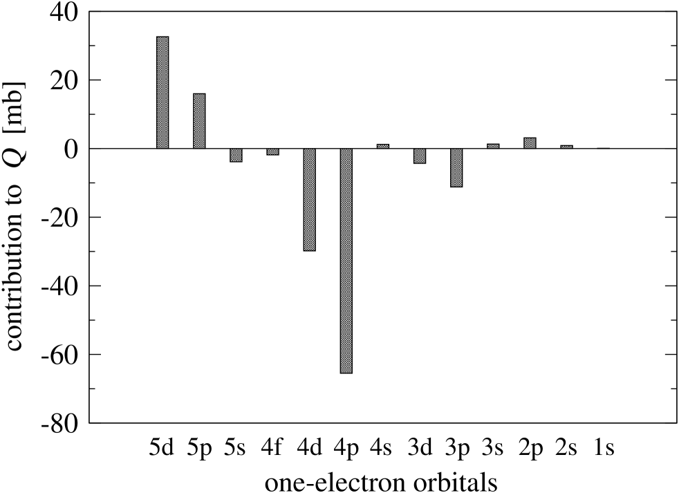
Figure 1: Contributions from occupied orbitals to the calculated value of $Q$ for the $5d^{9}6s^{2}$ ${}^{2}D_{3/2}$ state of Au. See caption of the Table 3 and Sec. III.2 for further details.

Table 3: Contributions from occupied orbitals to the calculated values of $A$ and $Q$ for the $5d^{9}6s^{2}$ ${}^{2}D_{3/2}$ state of Au; $orbitals$ = set of orbitals open for single and restricted double substitutions from all shells listed in the first column to the full virtual set; NCF = size of the multiconfiguration expansion; $\Delta$A = contribution [MHz] of the leftmost orbital from a given orbital set to the total $A$ value (i.e. the individual contribution of the $1s$ orbital is listed in the line $1s..6s$); $\Delta$Q = contribution [mb] of the leftmost orbital from a given set to the $Q$ value.

orbitals	NCF	$A$[MHz]	$\Delta$A	$Q$[mb]	$\Delta$Q
—	1	$218.011$	—	$580.807$	—
5d6s	16457	$189.406$	$-$28.605	$613.418$	32.611
5pd6s	39808	$153.103$	$-$36.302	$629.418$	16.000
5spd6s	48129	$190.849$	37.746	$625.559$	$-$3.859
4f5spd6s	89477	$187.661$	$-$3.188	$623.738$	$-$1.821
4df5spd6s	124673	$194.614$	6.953	$593.938$	$-$29.800
4pdf5spd6s	148188	$202.721$	8.107	$528.442$	$-$65.496
4spdf5spd6s	156525	$196.476$	$-$6.245	$529.646$	1.204
3d4spdf5spd6s	191721	$199.346$	2.870	$525.342$	$-$4.304
3pd…6s	215236	$201.106$	1.760	$514.175$	$-$11.167
3spd…6s	223573	$199.872$	$-$1.234	$515.495$	1.320
2p3spd…6s	247088	$196.564$	$-$3.308	$518.635$	3.140
2sp3spd…6s	255425	$199.576$	3.012	$519.539$	0.904
1s2sp3spd…6s	263762	$199.554$	$-$0.022	$519.634$	0.095

A similar procedure has been carried out for the $Q$ and $A$ values of the $5d^{9}6s^{2}$ ${}^{2}D_{5/2}$ state. The results for the ${}^{2}D_{5/2}$ state are shown in table 4 and in figure 2. The individual contributions of the $2p$, $2s$, and $1s$ orbitals to the total $Q$ value were of the order of 0.5 %, 0.2 %, and 0.02 %, respectively. The combined contribution of $1s2sp$ shells was of the order of 0.7 %, with respect to the total $Q$ value.

All these contributions have been included in the $Q$ and $A$ values obtained within the SrD approximation and the configuration state functions (CSFs) involved in evaluation of these contributions were carried over to all subsequent calculations.

It should be pointed out that the data in Tables 3 and 4 and in the Figures 1 and 2 were obtained with single and restricted double substitutions, i.e., with unrestricted double and triple substitutions excluded. Therefore the contributions of the $5psd$ and $4spdf$ shells are somewhat distorted — if double and triple substitutions were included, the individual contributions of the $5psd$ and $4spdf$ shells would differ by a few percent. Only the $3spd$, $2sp$ and $1s$ shells are essentially insensitive to double and triple substitutions (see Sec. III.3 below). Therefore their contributions are approximately correct.

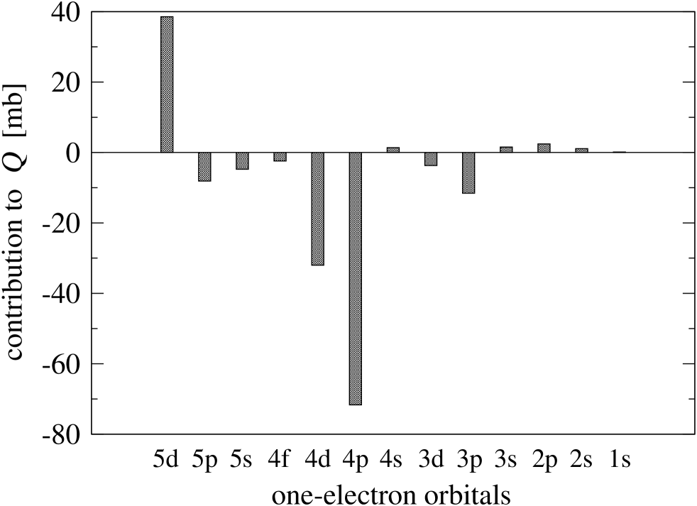
Figure 2: Contributions from occupied orbitals to the calculated value of $Q$ for the $5d^{9}6s^{2}$ ${}^{2}D_{5/2}$ state of Au. See caption of Table 4 and Sec. III.2 for further details.

Table 4: Contributions from occupied orbitals to the calculated values of $A$ and $Q$ for the $5d^{9}6s^{2}$ ${}^{2}D_{5/2}$ state of Au; $orbitals$ = set of orbitals open for single and restricted double substitutions from all shells listed in the first column to the full virtual set; NCF = size of the multiconfiguration expansion; $\Delta$A = contribution [MHz] of the leftmost orbital from a given orbital set to the total $A$ value (i.e. the individual contribution of the $1s$ orbital is listed in the line $1s..6s$); $\Delta$Q = contribution [mb] of the leftmost orbital from a given set to the $Q$ value.

orbitals	NCF	$A$[MHz]	$\Delta$A	$Q$[mb]	$\Delta$Q
—	1	$79.041$	—	$612.985$	—
5d6s	21501	$106.724$	27.683	$651.547$	38.562
5pd6s	51800	$109.554$	2.830	$643.451$	$-$8.096
5spd6s	62536	$71.472$	$-$38.082	$638.694$	$-$4.757
4f5spd6s	117626	$70.636$	$-$0.836	$636.280$	$-$2.414
4df5spd6s	163739	$73.490$	2.854	$604.280$	$-$32.000
4pdf5spd6s	194221	$74.597$	1.107	$532.632$	$-$71.648
4spdf5spd6s	204973	$79.767$	5.170	$534.008$	1.376
3d4spdf5spd6s	251086	$80.877$	1.110	$530.308$	$-$3.700
3pd…6s	281568	$80.580$	$-$0.297	$518.734$	$-$11.574
3spd…6s	292320	$82.136$	1.556	$520.259$	1.525
2p3spd…6s	322802	$81.700$	$-$0.436	$522.677$	2.418
2sp3spd…6s	333554	$78.995$	$-$2.705	$523.757$	1.080
1s2sp3spd…6s	344306	$79.025$	0.030	$523.880$	0.123

III.3 Double, triple, and quadruple substitutions

The decomposition of the electron correlation correction to the hyperfine structure into one-, two-, three-, and four-body effects can be understood from the following (simplified) analysis. The structure of the $5d^{9}6s^{2}$ ${}^{2}D$ states of gold is determined to a large extent by the interaction of the valence $6s^{2}$ shell with a highly polarisable $5d^{9}$ shell. The direct and indirect effects of relativity bring the outer $d$ shell much closer, radially and energetically, to the valence $s$ orbital than in homologous silver and copper atoms Pyykkö (1988, 2004). This in turn increases the polarisation of the $5d^{9}$ shell by the valence electrons. Therefore, the core-valence interaction (the leading electron correlation correction) leads to the contraction of the $6s$ orbital, which overestimates the hyperfine structure. The unrestricted double substitutions affect the hyperfine structure in two ways: directly through the configuration state functions (CSFs) themselves but also indirectly through the change of the expansion coefficients of the important configurations obtained by single substitutions. Three-particle effects in turn affect the expansion coefficients of the configurations obtained from double substitutions. In a simple picture we can describe the wave function in terms of pair-correlation functions and the three-particle effects then account for polarisation of pair-correlation functions, leading to an increase of the hyperfine structure Jönsson et al. (1996b). Four-particle effects affect mostly the expansion coefficients of the configurations obtained from double substitutions. Therefore their influence on the hyperfine structure is indirect and second-order to that of the double substitutions. They are usually small and can often be neglected Godefroid et al. (1997); they are discussed in Sec. III.3.

Tables 5 and 6 show the results of configuration-interaction calculations, where various combinations of occupied and virtual sets were tested with single and unrestricted double substitutions. The data from both tables are also presented as empty circles in Fig. 3.

Table 5: Values of $Q$ and $A$ for the $D_{3/2}$ state, calculated in configuration-interaction approach, with single and unrestricted double substitutions, in several different multiconfiguration expansions; $from$ – spectroscopic orbitals opened for substitutions; $to$ – virtual orbital set; NCF – number of configurations; see text for further details.

experiment			$199.8425(2)$
from	to	NCF	$A$[MHz]	$Q$[mb]
5spd6s	1spdfgh	259135	$205.426$	$521.191$
4spdf5spd6s	1spdfgh	358019	$205.968$	$521.503$
5spd6s	2spdf	279559	$210.523$	$509.839$
5spd6s	2spdfg	320545	$211.512$	$511.461$
5spd6s	2spdfgh	366257	$211.480$	$512.286$
5spd6s	3spdf2g1h	459594	$213.088$	$510.451$
5spd6s	3spdf2gh	465794	$213.075$	$510.402$
5spd6s	3spdfg2h	506987	$213.146$	$510.268$
5spd6s	4spdf2gh	687301	$213.200$	$510.478$

Table 6: Values of $Q$ and $A$ for the $D_{5/2}$ state, calculated in configuration-interaction approach, with single and unrestricted double substitutions, in several different multiconfiguration expansions; $from$ – spectroscopic orbitals opened for substitutions; $to$ – virtual orbital set; NCF – number of configurations; see text for further details.

experiment			$80.236(3)$
from	to	NCF	$A$[MHz]	$Q$[mb]
5spd6s	1spdfgh	339306	$74.258$	$507.823$
4spdf5spd6s	1spdfgh	467381	$72.048$	$509.321$
5spd6s	2spdfgh	480824	$73.468$	$512.278$
5spd6s	3spdf2gh	607421	$73.494$	$512.559$
5spd6s	4spdf3gh	898368	$73.294$	$514.621$
5spd6s	5spdf4g3h	1228675	$73.212$	$514.269$

Table 7: Values of $Q$ and $A$ for the $D_{3/2}$ state, calculated in configuration-interaction approach, with single and unrestricted double and triple substitutions, in several different multiconfiguration expansions; $from$ – spectroscopic orbitals opened for substitutions; $to$ – virtual orbital set; NCF – number of configurations; see text for further details.

experiment			$199.8425(2)$
from	to	NCF	$A$[MHz]	$Q$[mb]
5spd6s	1spd	265183	$198.955$	$520.346$
5spd6s	1spdf	386326	$194.391$	$533.464$
5spd6s	1spdfg	641227	$193.744$	$536.620$
5spd6s	1spdfgh	1012615	$193.246$	$537.786$
5spd6s	2spd1f	943544	$198.752$	$522.361$
5spd6s	2spdf	1543051	$199.973$	$520.536$
5spd6s	3spd2f	1200261	$198.207$	$520.267$
5spd6s	3psdf	1309130	$198.254$	$520.096$

Table 8: Values of $Q$ and $A$ for the $D_{5/2}$ state, calculated in configuration-interaction approach, with single and unrestricted double and triple substitutions, in several different multiconfiguration expansions; $from$ – spectroscopic orbitals opened for substitutions; $to$ – virtual orbital set; NCF – number of configurations; see text for further details.

experiment			$80.236~{}(3)$
from	to	NCF	$A$[MHz]	$Q$[mb]
5spd6s	1spd	341440	$81.6955$	$514.929$
5spd6s	1spdf	456506	$82.1357$	$520.259$
4f5spd6s	1spdf	1403860	$79.9343$	$518.380$
5spd6s	1spdfg	842883	$80.2371$	$519.291$
5spd6s	2spdf	1326851	$83.0623$	$521.862$

Table 9: Values of $Q$ and $A$ for the $D_{3/2}$ state, calculated in configuration-interaction approach, with single and unrestricted double, triple, and quadruple substitutions, in several different multiconfiguration expansions; $type$ – substitution multiplicity; $from$ – spectroscopic orbitals opened for substitutions; $to$ – virtual orbital set; NCF – number of configurations; see text for further details.

experiment			199.8425(2)
type	from	to	NCF	$A$[MHz]	$Q$[mb]
SDT	5spd6s	1spd	386326	$194.391$	$533.464$
SDTQ	5spd6s	1spd	569497	$194.301$	$533.653$
SDT	5spd6s	1spdf	386326	$194.391$	$533.464$
SDTQ	5spd6s	1spdf	967871	$195.376$	$531.685$
SDTQ	5spd6s	1spdf	1089014	$194.686$	$531.846$

The second line in Tables 5 and 6 represents a calculation in which substitutions from the $4spdf$ shells were allowed to one layer of virtual orbitals. When compared with the first line, it yields the effect of $4spdf$ shells on the calculated values of $Q$ and $A$. In order to limit the size of the configuration expansions, the CSFs representing the above substitutions were not carried over to the following, higher order calculations. Instead, the corrections were included additively, as described in Sec. IV.1. At the same time the evaluation of these corrections may be treated as a crude estimate of error arising from omitted double substitutions from occupied shells (see Sec. IV.2 for details).

An inspection of the last column of Table 5 indicates, that three layers of virtual orbitals were necessary to reach convergence of the $Q$ and $A$ values in the single and unrestricted double substitutions (SD) approximation for the $5d^{9}6s^{2}$ ${}^{2}D_{3/2}$ state. Four layers were necessary in case of the $5d^{9}6s^{2}$ ${}^{2}D_{5/2}$ state (see Table 6).

Tables 7 and 8 show the results of configuration-interaction calculations, in which various combinations of occupied and virtual sets were tested with unrestricted double and triple substitutions. The data from both tables are also presented as full circles in Fig. 3. Two layers of virtual orbitals were necessary to reach convergence of the $Q$ value in the single and double and triple substitutions (SDT) approximation for both $5d^{9}6s^{2}$ ${}^{2}D_{3/2}$ and $5d^{9}6s^{2}$ ${}^{2}D_{5/2}$ states. In case of the $A$ values, convergence required three, rather than two, layers.

Table 9 shows the effect of quadruple substitutions. The first line represents an approximation in which single, double, and triple substitutions from $5spd6s$ orbitals to a truncated virtual layer composed of ’s’, ’p’, and ’d’ symmetries were included. The third line represents a similar approximation in which the (still truncated) virtual layer was composed of ’s’, ’p’, ’d’, and ’f’ symmetries. The second, fourth, and fifth lines represent corresponding ’quadruple approximation’ in which single, double, triple, and quadruple substitutions were allowed. The comparison had to be made on a reasonably small orbital set in order to be able to converge the calculation involving quadruple substitutions. The numbers of CSFs in the last two lines are different, because certain restrictions were applied in the calculation represented by the fourth line (see the comments near the end of Sec. III.4 for details). The results presented in the table 9 indicate that the correction involving quadruple substitutions is unlikely to exceed 1 %. The CSFs representing quadruple substitutions were not carried over to the following calculations and the ’quadruple’ correction was included additively, as described in Sec. IV.1.

III.4 4-D configuration-interaction calculations

A full, converged Complete Active Space (CAS) calculation for the gold atom is still unattainable due to software and hardware limitations. Based on our current calculations we estimate that the CAS approach would require configuration expansions in four ’dimensions’: (1) single, double, triple, and perhaps quadruple substitutions; (2) from all core shells (or at least from $3spd4spdf5spd6s$); (3) to eight or more virtual orbital layers; (4) of $s$, $p$, $d$, $f$, $g$, $h$, and perhaps higher symmetries. One can imagine a ’space’ spanned by the four ’dimensions’ defined above, i.e. ’substitution multiplicity’, ’number of opened core subshells’, ’number of virtual layers’, and ’maximal symmetry of virtual layers’ dimension. In fact, this space should rather be called a ’matrix’, since all four dimensions are discrete. Let’s call this four-dimensional matrix a ’CAS matrix’. Each element of the matrix is represented by a multiconfiguration expansion obtained by substituting a particular number of electrons (’substitution’ dimension) from specific core orbitals (’core’ dimension) to a set of virtual orbitals (’virtual’ dimension) of specific symmetries (’symmetry’ dimension). A full CAS calculation would require several orders of magnitude larger configuration expansions than are possible even with the largest computer resources available today.

Table 10: The final configuration-interaction calculations of $Q$ and $A$ for the $5d^{9}6s^{2}$ ${}^{2}D_{3/2}$ state of Au; $type$ — description of the multiconfiguration expansions, see text for details; NCF = size of the multiconfiguration expansion.

experiment		$199.8425(2)$
type	NCF	$A$[MHz]	$Q$[mb]
SD:3hgg ​​​ + SDT:2fd	1182329	$206.343$	$517.201$
SD:3hgf + SDT:2fd	1144532	$206.221$	$517.342$
SD:3hgf + SDT:2gd	1711382	$205.104$	$519.106$
SD:3hgf + SDT:2gf	1847380	$204.489$	$519.829$

Table 11: The final configuration-interaction calculations of $Q$ and $A$ for the $5d^{9}6s^{2}$ ${}^{2}D_{5/2}$ state of Au; $type$ — description of the multiconfiguration expansions, see text for details; NCF = size of the multiconfiguration expansion.

experiment		$80.236~{}(3)$
type	NCF	$A$[MHz]	$Q$[mb]
SD:3hgf + SDT:2fd	1441120	$78.2451$	$520.073$
SD:3hgf + SDT:2gd	1527668	$79.9182$	$522.066$

However, a computational strategy can be designed in which a considerably smaller multiconfiguration expansion yields a wave function only marginally inferior to a full CAS wave function, in the sense that all important electron correlation effects are included and the calculated values of $A$ and $Q$ are close to those that would result from a full, converged, CAS calculation. The strategy is based on the observation that one does not have to simultaneously push the configuration expansions to the limits of all the above mentioned ’dimensions’. Specifically, the dependence of atomic properties on the ’substitution’ dimension is critical. To illustrate this approach, let’s consider separately the contributions of single, double, and triple substitutions to the calculated values of $A$ and $Q$ of gold. To obtain converged results within a single substitutions model, one has to include substitutions from all occupied shells ($1s2sp3spd4spdf5spd6s$) to eight or more virtual layers. This is illustrated in tables 1, 2, 3, and 4, where eight virtual orbital layers were necessary to converge the series of self-consistent-field calculations. However, to obtain a converged result within a single and double substitutions model (SD) one has to include double substitutions from $4spdf5spd6s$ occupied orbitals, not to eight, but to three or at most four virtual layers (see Tables 5 and 6). In the single, double, and triple substitutions model (SDT) it is enough to consider triple substitutions from $5spd6s$ occupied orbitals to two or at most three virtual layers (see Tables 7 and 8). In the ’space’ (or rather in the ’matrix’) of the four ’dimensions’ defined above, the ’core’ and ’virtual’ dimension sizes strongly depend on the ’substitution’ dimension (in fact, all four dimensions are interdependent).

Therefore, one can construct an approximation, in which all important electron correlation effects are included and the calculated values of $A$ and $Q$ are close to those that would result from a full, converged CAS calculation. In order to find a suitable approximation, we have performed a set of test calculations for several elements of the above mentioned ’matrix’. For each ’dimension’, the calculations were saturated to the point where the relative change of the expectation values (i.e., both $A$ and $Q$) did not exceed a small fraction of a percent (usually two or three tenths of a percent). Specifically, for each ’substitution’ dimension (i.e., for single, double, and triple substitutions) we thoroughly tested the dependence of observables on ’symmetry,’ ’virtual’, and ’core’ spaces. When a saturated set of configuration state functions (CSFs) is obtained for a particular ’substitution’ dimension, all these CSFs are carried over to the next step(s). The merged, ’final’ multiconfiguration expansion represents an approximation, which is effectively equivalent to a CAS expansion, and the corresponding wavefunction is of similar quality as a CAS wavefunction, at least from the point of view of the calculated values of $A$ and $Q$.

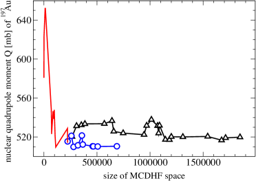
(a)  from electric field gradient and B($5d^{9}6s^{2}$ ${}^{2}D_{3/2}$)

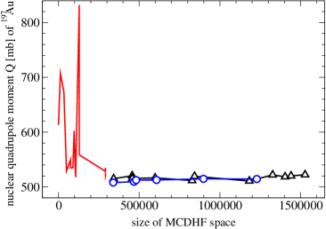
(b)  from electric field gradient and B($5d^{9}6s^{2}$ ${}^{2}D_{5/2}$)

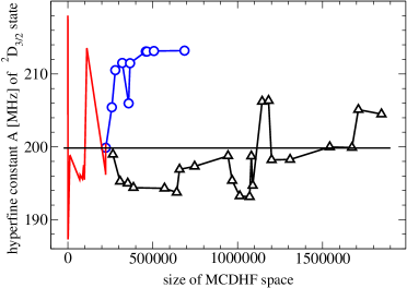
(c)  A($5d^{9}6s^{2}$ ${}^{2}D_{3/2}$)

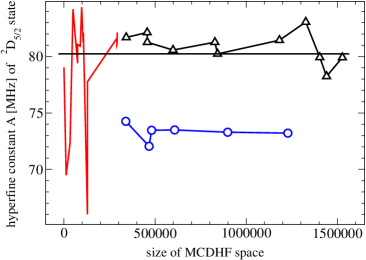
(d)  A($5d^{9}6s^{2}$ ${}^{2}D_{5/2}$)

Figure 3: (Color online) Nuclear quadrupole moment $Q$(${}^{197}\!$Au) [mb] obtained from the calculated electric field gradients, and hyperfine magnetic dipole constants $A$ [MHz] of the states $5d^{9}6s^{2}$ ${}^{2}D_{3/2}$ and $5d^{9}6s^{2}$ ${}^{2}D_{5/2}$, as functions of the size of the multiconfiguration expansions; line with no symbols (red online) – ’SrD’ approximation; circles (blue online) – ’SD’ approximation; triangles (black online) – ’SDT’ and final ’CAS’ approximations (see text for details). Horizontal straight lines in figures (c) and (d) represent the experimental values of hyperfine constants $A(^{2}D_{3/2})$ = 199.8425(2) MHz Blachman et al. (1967) and $A(^{2}D_{5/2})$ = 80.236(3) MHz Childs and Goodman (1966), respectively. The small corrections described in subsection IV.1 are not included in the figures.

In practice there is not one single final ’CAS’ expansion, but a series of such final expansions in which various sets of ’S’, ’SD’, and ’SDT’ multiconfiguration expansions (i.e. various sets with single, double, and triple substitutions) are merged together. Table 10 shows the results obtained from a series of such final ’CAS’ calculations for the ${}^{2}D_{3/2}$ state, and Table 11 shows the same for the ${}^{2}D_{5/2}$ state. The data from both tables are also included in Fig. 3. The ’CAS’ expansions are composed as follows. All virtual orbitals and all CSFs generated in the SrD approximation, as described in section III.1, as well as those described in section III.2, were included. The remaining CSF expansions were generated with substitutions from $5spd6s$ orbitals to virtual sets described in the first column of Tables 10 and 11, where symbols before the colon represent substitution multiplicity, i.e., SD — single and double substitutions; SDT — single and double and triple substitutions; the symbols after the colon represent virtual orbital layers, i.e., 3hgg — three layers (first layer with ’spdfgh’ symmetries and two layers with ’spdfg’ symmetries); 2fd — two layers (first layer with ’spdf’ symmetries and second layer with ’spd’ symmetries); 3hgf — three layers (first layer with ’spdfgh’ symmetries, second layer with ’spdfg’ symmetries; third layer with ’spdf’ symmetries), etc.

In the largest calculations, when single, double, and triple substitutions to two or three layers were included, we had to further limit the overall number of CSFs, due to software and hardware limitations. In those cases, the occupation number of the least important virtual orbital was restricted to single or double, thus excluding those CSFs in which this particular virtual orbital was occupied by three electrons. The difference that such a restriction brings about can always be evaluated on a smaller set of CSFs before a full calculation is performed. Therefore we always had control on the effects of the above mentioned restrictions on the calculated values of $A$ and $Q$.

IV Results

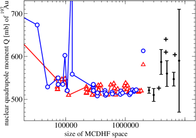
Figure 4: (Color online) Nuclear quadrupole moment $Q$ [mb] of the ${}^{197}\!$Au isotope obtained from the calculated electric field gradients, as a function of the size of multiconfiguration expansions for the states $5d^{9}6s^{2}$ ${}^{2}D_{3/2}$ (triangles – red online) and $5d^{9}6s^{2}$ ${}^{2}D_{5/2}$ (circles – blue online), compared with other theoretical and experimental results. The small corrections described in subsection IV.1 are not included in the figure. The values which represent multiconfiguration expansions of sizes smaller than 20000 are outside the figure, except the uncorrelated Dirac-Hartree-Fock values, represented by the single triangle (red online) for ${}^{2}D_{3/2}$ and the single circle (blue online) for ${}^{2}D_{5/2}$. The six values with error bars are from references Yakobi et al. (2007); Belpassi et al. (2007); Itano (2006); Palade et al. (2003); Powers et al. (1974); Childs and Goodman (1966); the four values without error bars, represented by pluses, are from references Thierfelder et al. (2007); Schwerdtfeger et al. (2005); Blachman et al. (1967); all data are arranged in reverse chronological order, with the most recent results to the left.

More extensive calculations turned out to be beyond the 100 node limit for this project on the Linux cluster at the National Institute of Standards and Technology (NIST), USA. Therefore the calculations of the magnetic dipole constants $A$ did not yield converged results. As might be expected, the effects of double and triple substitutions are relatively larger for $A$ than for $Q$, therefore the calculations of the $Q$ values were essentially converged; they yield: Q(${}^{2}D_{3/2}$) = 519.829 mb, and Q(${}^{2}D_{5/2}$) = 522.066 mb, respectively.

IV.1 Corrections

As mentioned in section III.3, the contributions arising from unrestricted double substitutions from $4spdf$ orbitals were evaluated separately and included additively in the final $Q$ values. They yield +0.312 mb and +1.498 mb for the two states ${}^{2}D_{3/2}$ and ${}^{2}D_{5/2}$, respectively. The effects of the quadruple substitutions were also evaluated separately, in a very limited fashion, and only for the ${}^{2}D_{3/2}$ state. As explained in section III.3, the correction arising from the quadruple substitutions for the ${}^{2}D_{3/2}$ state lowers the $Q$ value by 1.779 mb. The dependence of the $Q$ values on double and triple substitutions indicates that the quadruple correction might be smaller for the $Q(^{2}D_{5/2})$ value than for the $Q(^{2}D_{3/2})$ value, but we were unable to evaluate the former. Therefore we assumed identical, $-$1.8 mb corrections for both states. The corrections arising from the Breit interaction were calculated at the Dirac-Hartree-Fock level with full relaxation i.e. with a frequency-dependent Breit term

$$B_{ij} = -\frac{\bm{\alpha}_{i}\cdot\bm{\alpha}_{j}}{r_{ij}}-\frac{\bm{\alpha}_{i}\cdot\bm{\alpha}_{j}}{r_{ij}}[\cos(\omega_{ij}r_{ij})-1]$$ (3)

$$+c^{2}(\bm{\alpha}_{i}\cdot\vec{\nabla}_{i})(\bm{\alpha}_{j}\cdot\vec{\nabla}_{j})\frac{\cos(\omega_{ij}r_{ij}/c)-1}{\omega_{ij}^{2}r_{ij}}$$

included in the self-consistent-field functional, using the mcdfgme code Desclaux (1993); Indelicato (1995); Indelicato and Desclaux (2005). In the formula above, $r_{ij}=\left|\vec{r}_{i}-\vec{r}_{j}\right|$ is the inter-electronic distance, $\omega_{ij}$ is the energy of the photon exchanged between two electrons, $\bm{\alpha}_{i}$ are Dirac matrices, and $c=1/\alpha$ is the speed of light. The Breit corrections are highly state-dependent (see also Yakobi et al. (2007), where the Gaunt part was evaluated) and yield 2.3 mb and 0.6 mb for the two states, ${}^{2}D_{3/2}$ and ${}^{2}D_{5/2}$, respectively. The quantum electrodynamics (QED) corrections to the $Q$ values are expected to be very small. We evaluated the VP (vacuum polarisation) correction with the mcdfgme code, following Ref. Boucard and Indelicato (2000), and obtained a value of the order of 0.01 %. When all above mentioned corrections are included, the $Q$ values become: Q(${}^{2}D_{3/2}$) = 520.641 mb and Q(${}^{2}D_{5/2}$) = 522.364 mb. The average of the above two results yields Q(${}^{197}\!$Au) = 521.5 mb.

IV.2 Error estimate

A rigorous, systematic treatment of the error bar of the calculated electric quadrupole moment $Q$ would require evaluation of the effects of: all omitted virtual orbitals, all CSFs which were not included in the configuration expansions, as well as all physical effects that were not included or were treated approximately. However, we were only able to obtain very crude estimates of certain sources of systematic errors. We believe that none exceeded 1 %, but the calculations presented in this paper were far too extensive to permit a rigorous treatment of the error. Therefore we have to resort to a less rigorous method.

One of the frequently used methods of evaluation of the accuracy of calculated electric quadrupole moments $Q$ is based on the simultaneous calculations of magnetic dipole hyperfine constants $A$, and on subsequent comparison of calculated $A$ values with their experimental counterparts. As mentioned above, the calculations of the magnetic dipole constants $A$ have not converged. However, the amplitudes of the final oscillations of the two curves representing the values of $A$ for the two states of interest are comparable to the uncertainty of $A$ arising from the accuracy of the nuclear magnetic dipole moment value $\mu$.

There are currently two different $\mu$ values in the literature Raghavan (1989); Stone (2005), $\mu$ = 0.145746(9) and $\mu$ = 0.148158(8), which differ by about 2 %. Taken at face value, our results seem to favor the smaller value, $\mu$ = 0.145746(9), which, as mentioned in Sec. II, has been used in the present calculations. However, the overall accuracy of our calculations (in particular, the evaluation of higher-order terms) does not permit us to draw a definitive conclusion. Therefore, the difference between the two values of $\mu$ should rather be treated as a source of systematic error in the determination of $A$. Therefore, we did not push the calculations of magnetic dipole constants $A$ further beyond their current level of convergence and, consequently, the calculations of $A$ values could not be used as reliable sources of error estimate for nuclear moments.

Another method to estimate the accuracy of $Q$ is to consider the differences between the final values obtained from different states. However, in the present paper we were able to converge the calculations for only two atomic levels. The difference between the results obtained for these two levels turned out to be quite small, which rendered this method useless in this particular case.

Considering the computational methodology employed in this paper, it is obvious that the final value depends on the choice of the multiconfiguration expansions representing the last few points on the curves in Fig. 4, while the accuracy of the final value is connected with convergence of these curves. Therefore, we based the estimate of the error bar on the oscillations of the tail of the two curves in Fig. 4. The largest difference taken from the last few points on the curves representing ${}^{2}D_{3/2}$ and ${}^{2}D_{5/2}$ states amounts to 3 mb and 4 mb, respectively. As an additional source of uncertainty we assumed the additive corrections described in subsection IV.1, since all of them were evaluated in a rather crude approximation. For instance, the contribution of the Breit interaction was calculated at the Dirac-Hartree-Fock level, without regard for electron correlation effects. When all above sources of uncertainly are taken into account the total error bar amounts to 5 mb, which yields our final calculated value of quadrupole moment Q(${}^{197}\!$Au) = 521.5 $\pm$ 5.0 mb.

V Comparisons

The results of our calculation are compared with previous evaluations in Table 12 and in Fig. 4. It is worth noting that our result is in agreement with three most recent theoretical values, obtained with three different methods, but all these recent results (including ours) are considerably smaller than other, earlier values.

Yakobi et al Yakobi et al. (2007) performed calculations for the $5d^{9}6s^{2}$ ${}^{2}D_{3/2}$ and $5d^{9}6s^{2}$ ${}^{2}D_{5/2}$ states of atomic gold within the four-component Dirac-Coulomb framework Eliav et al. (1994); Kaldor and Eliav (1998). They correlated 51 out of the 79 electrons in the large basis sets (up to 26s22p18d12f8g5h uncontracted Gaussian functions) with the relativistic Fock-space coupled cluster method, including single and double excitations (CCSD). The contribution of the Gaunt term, the main part of the Breit interaction, was also evaluated.

Belpassi et al Belpassi et al. (2007) performed molecular relativistic Dirac-Coulomb-Gaunt Hartree-Fock calculations Pernpointner and Visscher (2001) for a series of molecules: AuF, XeAuF, KrAuF, ArAuF, (OC)AuF, and AuH. The electronic correlation contributions were included at CCSD(T) and CCSD-T levels. The value of the nuclear quadrupole moment $Q$ was obtained from the determinations of the electric field gradient at the gold nucleus for the above mentioned molecules, combined with experimental values of the nuclear quadrupole coupling constants.

Thierfelder et al Thierfelder et al. (2007) performed four-component relativistic density-functional (DFT) calculations for diatomic compounds CuX and AuX (X = H, F, Cl, Br, and I) with and without CO attached, i.e., OC-CuX and OC-AuX (X = F, Cl, Br, and I). They employed a newly developed functional Yanai et al. (2004), whose role is to correctly describe the long-range part of exchange interactions Goll et al. (2007), and obtained the averaged result Q = 526 mb. This value is within the error bounds of our value.

Our result, in turn, falls within the error bounds published by Belpassi et al (Q = 510(15) mb), as well as those by Yakobi et al (Q = 521(7) mb). The agreement with Yakobi et al may be somewhat accidental because particular contributions show larger differences. The two outstanding differences arise from triple substitutions and from deep core orbitals. Yakobi et al evaluated the effect of the triple substitutions by performing single-reference CCSD(T) calculation for the ${}^{2}D_{5/2}$ level, and obtained a 0.3 % shift. The effect of triple substitutions is indeed smaller for the ${}^{2}D_{5/2}$ level, but for the ${}^{2}D_{3/2}$ level our calculations indicate a shift of the order of 2 %. However, this discrepancy may be attributed to the methodological differences in the two papers. The definition of triple substitutions in the configuration-interaction method used here differs substantially from that in the CCSD(T) approach, due to the exponential nature of the coupled-cluster operator. The coupled-cluster approximation includes a subset of the CI triple substitutions (the ”unlinked” diagrams), as well as that of higher order substitutions, already at the CCSD level. The CCSD(T) yields only the ”linked” part as the effect of the triple substitutions. Therefore, the contribution of the CI triple substitutions may indeed be expected to be larger than that of the CC triple substitutions.

Another difference arises from contributions of deep core orbitals. The effects of $3spd$, $2sp$, and $1s$ orbitals were neglected by Yakobi et al, while in our calculations they were all included. Their combined effect was to lower the $Q$ value by about 2 %.

Table 12: Comparison of the present $Q$(¹⁹⁷Au) value (in mb = 10^-31 m²) with other recent values and with previous (muonic) standard value.

Reference	Source	Q(${}^{197}\!$Au)
This work	Au atom, ${}^{2}D_{3/2}$, ${}^{2}D_{5/2}$	521.5$\pm$5.0
Yakobi et al Yakobi et al. (2007)	Au atom, ${}^{2}D_{3/2}$, ${}^{2}D_{5/2}$	521$\pm$7
Belpassi et al Belpassi et al. (2007)	AuF, LAuF molecules	510$\pm$15
Thierfelder et al Thierfelder et al. (2007)	AuX, LAuX molecules	526
Powers et al Powers et al. (1974)	Muonic	547$\pm$16

Conclusions

The multiconfiguration Dirac-Hartree-Fock (MCDHF) model has been employed to calculate the expectation values responsible for the hyperfine splittings of the $5d^{9}6s^{2}$ ${}^{2}D_{3/2}$ and $5d^{9}6s^{2}$ ${}^{2}D_{5/2}$ levels of atomic gold. To our knowledge, this is the first calculation in which one-, two-, and three-body electron correlation effects were included and saturated for electric quadrupole hyperfine values of a heavy, open-shell, neutral atom. The correlation effects involving all 79 electrons were accounted for with a procedure that is equivalent to a full Complete Active Space calculation. All electron correlation effects were explicitly accounted for at a 1 % level of precision or better. Calculated electric field gradients, together with experimental values of the electric quadrupole hyperfine structure constants $B$, allow us to extract a nuclear electric quadrupole moment $Q$ = 521.5(5.0) mb of ¹⁹⁷Au. If taken at face value, the summary in table 12 suggests that our $Q$ value, together with that of Yakobi et al Yakobi et al. (2007), could be the new standard value.

References

- Jönsson et al. (2007) P. Jönsson, X. He, C. Froese Fischer, and I. P. Grant, Comput. Phys. Commun. 177, 597 (2007).
- Indelicato and Desclaux (2005) P. Indelicato and J.-P. Desclaux, Mcdfgme, a multiconfiguration dirac fock and general matrix elements program (release 2005), http://dirac.spectro.jussieu.fr/mcdf (2005).
- Desclaux (1975) J.-P. Desclaux, Computer Physics Communications 9, 31 (1975).
- Desclaux (1993) J.-P. Desclaux, in Methods and Techniques in Computational Chemistry, edited by E. Clementi (STEF, Cagliary, 1993), vol. A: Small Systems of METTEC, p. 253.
- Grant (2007) I. P. Grant, Relativistic Quantum Theory of Atoms and Molecules: Theory and Computation (Springer, New York, 2007).
- Lindgren and Morrison (1986) I. Lindgren and J. Morrison, Atomic Many-Body Theory (Springer-Verlag, New York Berlin Heidelberg, 1986).
- Dzuba (2005) V. A. Dzuba, Phys. Rev. A 71, 032512 (2005).
- Dzuba and Flambaum (2007) V. A. Dzuba and V. V. Flambaum, Phys. Rev. A 75, 052504 (2007).
- Johnson (2007) W. R. Johnson, Atomic Structure Theory: Lectures on Atomic Physics (Springer, Berlin, 2007).
- Bieroń et al. (1996) J. Bieroń, P. Jönsson, and C. Froese Fischer, Phys. Rev. A 53, 2181 (1996).
- Bieroń et al. (1999) J. Bieroń, P. Jönsson, and C. Froese Fischer, Phys. Rev. A 60, 3547 (1999).
- Yerokhin (2008) V. A. Yerokhin, Phys. Rev. A 77, 020501 (2008).
- Autschbach et al. (2002) J. Autschbach, S. Siekierski, M. Seth, P. Schwerdtfeger, and W. H. E. Schwarz, J. Comp. Chem. 23, 804 (2002).
- Malkin et al. (2004) I. Malkin, O. L. Malkina, V. G. Malkin, and M. Kaupp, Chem. Phys. Lett. 396, 268 (2004).
- Malkin et al. (2006) E. Malkin, I. Malkin, O. L. Malkina, V. G. Malkin, and M. Kaupp, Phys. Chem. Chem. Phys. 8, 4079 (2006).
- Song et al. (2007) S. Q. Song, G. F. Wang, A. P. Ye, and G. Jiang, J. Phys. B: At. Mol. Opt. Phys. 40, 475 (2007).
- Schwerdtfeger et al. (2005) P. Schwerdtfeger, R. Bast, M. C. L. Gerry, C. R. Jacob, M. Jansen, V. Kellö, A. V. Mudring, A. J. Sadlej, T. Saue, T. Söhnel, et al., J. Chem. Phys. 122, 124317 (2005).
- Itano (2006) W. M. Itano, Phys. Rev. A 73, 022510 (2006).
- Yakobi et al. (2007) H. Yakobi, E. Eliav, and U. Kaldor, J. Chem. Phys. 126, 184305 (2007).
- Belpassi et al. (2007) L. Belpassi, F. Tarantelli, A. Sgamellotti, H. M. Quiney, J. N. P. van Stralen, and L. Visscher, J. Chem. Phys. 126, 064314 (2007).
- Thierfelder et al. (2007) C. Thierfelder, P. Schwerdtfeger, and T. Saue, Phys. Rev. A 76, 034502 (2007).
- Pyykkö (2004) P. Pyykkö, Angew. Chem. Int. Ed. 43, 4412 (2004), edition in German: Angew. Chem. 116, 4512-4557 (2004).
- Pyykkö (2005) P. Pyykkö, Inorg. Chim. Acta 358, 4113 (2005).
- Pyykkö (2008a) P. Pyykkö, Chem. Soc. Rev. 37, 1967 (2008a).
- Pyykkö (2008b) P. Pyykkö, Mol. Phys. 106, 1965 (2008b).
- Grant (1994) I. P. Grant, Comput. Phys. Commun. 84, 59 (1994).
- Dyall et al. (1989) K. G. Dyall, I. P. Grant, C. T. Johnson, F. A. Parpia, and E. P. Plummer, Comput. Phys. Commun. 55, 425 (1989).
- Raghavan (1989) P. Raghavan, At. Data Nucl. Data Tables 42, 189 (1989).
- Stone (2005) N. J. Stone, At. Data Nucl. Data Tables 90, 75 (2005).
- Jönsson et al. (1996a) P. Jönsson, F. A. Parpia, and C. Froese Fischer, Comput. Phys. Commun. 96, 301 (1996a).
- Blachman et al. (1967) A. G. Blachman, D. A. Landman, and A. Lurio, Phys. Rev. 161, 60 (1967).
- Childs and Goodman (1966) W. J. Childs and L. S. Goodman, Phys. Rev. 141, 176 (1966).
- Bieroń et al. (2008) J. Bieroń, C. Froese Fischer, P. Jönsson, and P. Pyykkö, J. Phys. B: At. Mol. Opt. Phys. 41, 115002 (2008).
- Pyykkö (1988) P. Pyykkö, Chem. Rev. 88, 563 (1988).
- Jönsson et al. (1996b) P. Jönsson, A. Ynnerman, C. Froese Fischer, M. R. Godefroid, and J. Olsen, Phys. Rev. A 53, 4021 (1996b).
- Godefroid et al. (1997) M. Godefroid, G. V. Meulebeke, P. Jönsson, and C. Froese Fischer, Z. Phys. D 42, 193 (1997).
- Palade et al. (2003) P. Palade, F. E. Wagner, A. D. Jianu, and G. Filoti, J Alloys Comp. 353, 23 (2003).
- Powers et al. (1974) R. J. Powers, P. Martin, G. H. Miller, R. E. Welsh, and D. A. Jenkins, Nucl. Phys. A 230, 413 (1974).
- Indelicato (1995) P. Indelicato, Phys. Rev. A 51, 1132 (1995).
- Boucard and Indelicato (2000) S. Boucard and P. Indelicato, Eur. Phys. J. D 8, 59 (2000).
- Eliav et al. (1994) E. Eliav, U. Kaldor, and Y. Ishikawa, Phys. Rev. A 49, 1724 (1994).
- Kaldor and Eliav (1998) U. Kaldor and E. Eliav, Adv. Quantum Chem 31, 313 (1998).
- Pernpointner and Visscher (2001) M. Pernpointner and L. Visscher, J. Chem. Phys. 114, 10389 (2001).
- Yanai et al. (2004) T. Yanai, D. P. Tew, and N. C. Handy, Chem. Phys. Lett. 393, 51 (2004).
- Goll et al. (2007) E. Goll, H. Stoll, C. Thierfelder, and P. Schwerdtfeger, Phys. Rev. A 76, 032507 (2007).