Optimal effective current operator for flux qubit accounting for inductive effects

Abstract

An optimal effective current operator for flux qubit has been investigated by taking account of the inductive effects of the circuit loop. The whole system is treated as two interacting subsystems: one is the inductance-free flux qubit consisting of three Josephson junctions and the other a high frequency LC-oscillator. As the composite system hardly affords one excessively high energy LC photon, an effective theory for the inductive flux qubit providing its physical variable operators has been achieved, which can take account of the inductive effects but does not include the additional degree of freedom for the LC-oscillator. Considering the trade-off between simplicity and accuracy, it has been revealed that the optimal effective current operator resulting in an error only on the order of $L^{3/2}$ provides an approximation of high accuracy, which is also verified numerically.

I Introduction

Superconducting circuits are promising candidates for quantum information processingYGA2001 ; MAJ2004 ; Wendin2005 and, in order to reduce the impact of both charge and flux noise, flux qubit consisting of a superconducting loop interrupted by three Josephson junctions (3jj) has been proposed, designed and realized.TJL1999 ; JTL1999 ; CAF2000 ; IYC2003 ; IPK2004 ; WYJ2005 ; JPC2007 ; DMB2008 The loop in the original design is small enough and its inductive effects, therefore, could be neglected at the first approximation.TJL1999 The constraint of the flux quantization on the three phases across the 3jj yields two independent phase variables for the system. On the other hand, inductive effects are essential in several inductive coupling schemes JFA2005 ; JYF2005 ; Alec2005 ; MG2006 ; YLiu2006 ; YLiu2007 . These systems can be systematically studied by applying a general network graph theory GRD2004 ; GDP2005 , which indicates that an independent phase is associated to the loop self-inductance in the original circuit and the 3jj flux qubit, thus, turns out as a three-phase system. In order to include the inductive effects judiciously, appropriate terms could be reallocated to improve the original operators in the two-phase system. First, the inductive effects, considered as corrections to the energy levels of the two-phase system, have been addressed but with some flaws by Crankshaw et. al. in a semi-classical approachDT2001 , and, consequently, an effective Hamiltonian has been reachedAlec2005 as well as a current operator in the two-flux-state basis for the flux qubitYa2006 . Another reason why we build up an effective theory to include the inductive effects is that an inductance of a non-negligible size may lead the device to a less useful qubit.Robertson2006

Current operator is crucial to the accurate control, coupling and measurement of flux qubits.Lin2002 In particular, it could play a key role in understanding the dynamics of the flux qubit by a general multilevel model.WYJ2005 ; YJL2005 ; YWJ2005 Although various forms of current operators have been utilized in all kinds of regimes, the validity of the specific current operators has not been justified seriously and error analyses are hardly available. In this work, a systematic investigation on the optimal two-phase effective current operator for the three-phase system is carried out and an error analysis is provided.

The paper is organized as follows. In Sec.II, we review some basic ideas on the loop current in a classical circuit model. In Sec.III, we construct the three-phase Hamiltonian and decompose it into a form showing that two subsystems weakly interact with each other; then we develop an effective theory, the photon transition path (PTP) approach based on the Brillouin-Wigner expansionJJ1998 , to describe the three-phase system in Sec.IV. In Sec.V, we obtain the optimal effective two-phase loop current operator from the unique one for the whole system, and a brief numerical discussion is presented in Sec.VI.

II classical analysis

Figure 1: (a)circuit of an inductive flux qubit with the phase difference $\phi$ across the loop inductance $L$, the reduced applied external flux $\phi_{X}={2\pi\Phi_{X}}/{\Phi_{0}}$ with $\Phi_{0}$ the flux quantum, and the phase difference $\phi_{k}$ across the $k$th junction characterized via the critical current $I_{Ck}$ and the capacitance $C_{k}$ for $k$=1,2 and 3; (b) transformation between the current and voltage sources, the arrow and the plus/minus symbols indicate the directions of the current and voltage sources, respectively.

The schematic circuit for the 3jj flux qubit with a loop inductance is demonstrated in Fig. 1(a), where the 3rd junction is a little smaller than those two others; representing the relative sizes, the parameter $\alpha_{k}$ as

$$\alpha_{k} = \frac{I_{Ck}}{I_{C0}}=\frac{C_{k}}{C_{0}},k=1,2,3$$ (1)

indicates the area factor of the $k$th junction, where $I_{C0}=\left(I_{C1}+I_{C2}\right)/2$ and $C_{0}=\left(C_{1}+C_{2}\right)/2$ are design parameters. Parameters $\alpha_{1}$ and $\alpha_{2}$ are supposed to be close to 1, the deviations of which are determined by the accuracy of fabrication, while $\alpha_{3}\simeq 0.8$ and the reduced applied external flux $\phi_{X}$ is biased on the vicinity of $\phi_{X}=\pi$, all of which are selected to benefit the energy levels of the flux qubit. These three junction phases $\phi_{1,2,3}$ and the phase difference $\phi$ across the loop inductance $L$ are not independent of one another and obey the flux quantization in this superconducting system as

$$\phi_{1}+\phi_{2}+\phi_{3}=\phi+\phi_{X},$$ (2)

the signs of which are also indicated in Fig. 1(a).

In the classical regime, the junction performs as a current-flux 2-port circuit element, a nonlinear inductance, and the flux quantization condition imposes a predetermined constraint. In the DC regime, without considering capacitances, the loop current flows equivalently through four current elements in the loop including the Josephson junctions and the loop inductance as

$$I_{q}=I_{C_{k}}\sin\bar{\phi}_{k}=-\frac{\Phi_{0}}{2\pi}\frac{\bar{\phi}}{L},k=1,2,3,$$ (3)

where $\bar{\phi}_{1}$, $\bar{\phi}_{2}$, $\bar{\phi}_{3}$ and $\bar{\phi}$ are the possible static phase values obtained from Eqs. (2) and (3). Two opposite current directions present an additional degeneracy of the circuit. Furthermore, in the AC regime, if only taking account of the small oscillations in the circuit, each junction works at the static phase point as a pure inductance

$$L_{k}=\frac{\Phi_{0}}{2\pi I_{C_{k}}\cos\bar{\phi}_{k}}$$ (4)

if $\cos{\bar{\phi}_{k}}\neq 0$ for k=1,2 and 3. The series impedance of the circuit,

$$\mathbf{Z}(\omega)=-i\omega L+\sum_{k=1}^{3}\frac{-i\omega L_{k}}{1-\omega^{2}L_{k}C_{k}},$$ (5)

with $i$ the imaginary unit, provides its several characteristic frequencies; especially, when the circuit works at such an ultra-high frequency that the junction inductances can be treated as open circuits, there exists only one significant oscillation along the loop between its small inductance $L$ and series capacitance $C_{ser}$ with a high characteristic frequency

$$\omega_{LC}=\sqrt{\frac{1}{LC_{ser}}},$$ (6)

where $C_{ser}=(\sum_{k=1}^{3}C_{k}^{-1})^{-1}=\alpha_{ser}C_{0}$.

Generally, the nonlinear effects of the junctions generate current components of new frequencies different from the external flux-driven source’s. Only considering the output profiles of the junctions, we can still apply this kind of specific current sources to the rest of the circuit which obeys the linear superposition rules. Picking an arbitrary frequency $\omega$ in the frequency domain and utilizing a source transformation shown in Fig. 1(b), we have

$$I_{loop}(\omega)=\frac{\sum_{k=1}^{3}\frac{I_{Ck}(\omega)}{i\omega C_{k}}}{\sum_{k=1}^{3}\frac{1}{i\omega C_{k}}+i\omega L},$$ (7)

where $I_{Ck}(\omega)$ is obtained from $I_{Ck}\sin\phi_{k}$ via the Fourier transform. Interestingly, when $L$ is small enough to neglect, $I_{loop}(\omega)$ in Eq. (7) does not depend on $\omega$ explicitly and we utilize the inverse Fourier transform $\mathcal{F}^{-1}$ again as

$$I_{loop}(t)=\mathcal{F}^{-1}\left({I_{loop}(\omega)|_{\omega^{2}L\rightarrow 0}}\right)={C_{ser}}\sum_{k=1}^{3}\frac{I_{Ck}\sin\phi_{k}}{C_{k}},$$ (8)

where $\sum_{k=1}^{3}\phi_{k}=\phi_{X}$ since $\phi$ vanishes when $L\rightarrow 0$. This form of the loop current $I_{loop}(t)$ directly goes with the fact that the junctions connect to a topological network consisting of linear circuit elements. Delightfully, $I_{loop}(t)$ in Eq. (8) is in exact agreement with the one for the two-phase system derived in the quantum regime by Maassen van den BrinkAlec2005 and with our following effective one. This suggests that quantum superconducting circuit analysis and design might benefit in elegant ways from classical circuit theories and CAD tools.

III quantum analysis for system Hamiltonian

To construct the Hamiltonian comfortably, we firstly select three junction phases $\phi_{1,2,3}$ as the spatial variables and express the system Hamiltonian in a sum of energy terms similar to other superconducting loop circuits such as the RF-qubit and the SQUID-qubit as

$$\hat{H}_{3p}=\sum_{k=1}^{3}\left(\frac{\hat{Q}_{k}^{2}}{2C_{k}}-E_{Jk}\cos\hat{\phi}_{k}\right)+\left(\frac{\Phi_{0}}{2\pi}\right)^{2}\frac{\hat{\phi}^{2}}{2L},$$ (9)

where $\hat{Q}_{k}$ is the charge operator conjugated with the phase $\hat{\phi}_{k}$, i.e., $\hat{Q}_{k}=-2ei\frac{\partial}{\partial\phi_{k}}$ or $\left[\hat{\phi}_{k},\hat{Q}_{k}\right]=2ei$ with $e$ the electronic charge; $E_{Jk}=\frac{\Phi_{0}I_{Ck}}{2\pi}$ is the Josephson energy of the $k$th junction. The former sum in Eq.(9) represents the total energy of junctions including their charge and Josephson energy and the latter term the loop inductive energy. According to the design, the reduced inductance size $\beta$,

$$\beta = \frac{2\pi{L}I_{C0}}{\Phi_{0}},$$ (10)

is usually small enough that the loop phase difference $\hat{\phi}$ behaves as a small variable with its norm $\|\hat{\phi}\|$ tending to be equal to zero, while the loop current still keeps finite due to the biased junctions. Consequentially, its conjugate variable $\hat{Q}_{\phi}$, which we refer to as $\left[\hat{\phi},\hat{Q}_{\phi}\right]=2ei$, diverges on its norm according to the Heisenberg uncertainty principle $\|\hat{\phi}\|\bullet\|\hat{Q}_{\phi}\|\gtrsim{e}$. In the classical regime, a quadratic potential $\left(\frac{\Phi_{0}}{2\pi}\right)^{2}\frac{\phi^{2}}{2L}$ means that there is a generalized restoring force

$$\vec{F}_{osc} = \frac{\Phi_{0}}{4\pi L}\nabla_{\phi_{1},\phi_{2},\phi_{3}}\phi^{2}=\frac{\Phi_{0}\phi}{2\pi L}[1,1,1]^{T}$$ (11)

providing a non-parallel generalized acceleration

$$\vec{a}_{osc} = \mathbf{C}_{diag}^{-1}\vec{F}_{osc}=\frac{\Phi_{0}\phi}{2\pi LC_{0}}\vec{r},$$ (12)

where $\mathbf{C}_{diag}$ is a diagonal matrix with its diagonal elements being $C_{1}$,$C_{2}$ and $C_{3}$, and

$$\vec{r}=[\frac{1}{\alpha_{1}},\frac{1}{\alpha_{2}},\frac{1}{\alpha_{3}}]^{T}.$$

In the quantum regime, the deep quadratic potential explicitly in proportion to $1/\beta$ is capable to bind up the quantum states of this three dimensional system in the vicinity of a phase plane $\phi=0$, where a fast vacuum fluctuation occurs along the unique direction $\vec{r}$ parallel to the acceleration $\vec{a}_{osc}$. Therefore, the original spatial variable set ($\phi_{1}$,$\phi_{2}$,$\phi_{3}$), although helpful in the construction of the Hamiltonian, presents difficulties in handling the charge operator $\hat{Q}_{\phi}$, which represents one of the most important quantum properties of the three-phase system.

To solve the problem, we utilize a linear transformation to achieve another set of coordinates ($\phi$,$\theta_{1}$,$\theta_{2}$) where besides $\phi$ the other two coordinates are labeled via $\theta_{1}$ and $\theta_{2}$ and their conjugates are $\hat{Q}_{\theta_{1}}$ and $\hat{Q}_{\theta_{2}}$, respectively. The linear transformation between these two sets of coordinates is introduced via a matrix $\mathbf{A}$ defined as $[\theta_{1},\theta_{2},\phi+\phi_{x}]^{T}=\mathbf{A}[\phi_{1},\phi_{2},\phi_{3}]^{T}$, or equivalently as

$$\mathbf{\hat{Q}}_{\Theta}^{T}=\left[\hat{Q}_{\theta_{1}},\hat{Q}_{\theta_{2}},\hat{Q}_{\phi}\right]=\left[\hat{Q}_{1},\hat{Q}_{2},\hat{Q}_{3}\right]\mathbf{A}^{-1}.$$ (13)

Thus, the Hamiltonian $\hat{H}_{3p}$ changes to

$$\hat{H}_{A}=\frac{1}{2}\mathbf{\hat{Q}}_{\Theta}^{T}\mathbf{A}\mathbf{C}_{diag}^{-1}\mathbf{A}^{T}\mathbf{\hat{Q}}_{\Theta}+V(\theta_{1},\theta_{2},\phi),$$ (14)

where $V(\theta_{1},\theta_{2},\phi)$ is the potential in the new framework. Since the charge operator $\hat{Q}_{\phi}$ tends to diverge when $\beta\rightarrow 0$, if the charge coupling coefficients in $\mathbf{A}\mathbf{C}_{diag}^{-1}\mathbf{A}^{T}$ are assumed to be finite and independent of $\beta$, a proper candidate for $\Theta$-subsystem on ($\theta_{1},\theta_{2}$) should avoid any direct charge coupling from the $\phi$-subsystem. It mathematically requires that the directions of $\theta_{1}$ and $\theta_{2}$ in the original coordinates should be perpendicular to the acceleration direction $\vec{r}$ of the oscillation mentioned above, which means that the plane spanned by $\theta_{1}$ and $\theta_{2}$ is unique as well as

$$\hat{Q}_{\phi} = {C_{ser}}\sum_{k=1}^{3}\frac{\hat{Q}_{k}}{C_{k}},$$ (15)

revealing the charge in the series capacitor $C_{ser}$. Some other explanations in the classical regime are also given in Refs. Alec2005, and DT2001, , both of which have achieved the proper variable transformations by avoiding the cross charge energy terms between $\Theta$ and $\phi$ subsystems. Although they have predicted the right ones based on the linearity of the circuit, it is more comfortable in the quantum regime to emphasize the reason why the $\Theta$-subsystem as well as $\hat{Q}_{\phi}$ should be selected uniquely, since the diverging charge fluctuations merely serve as a pure quantum phenomenon.

The remaining degrees of freedom endowed by $\mathbf{A}$ involve the internal variable selections of $\Theta$-subsystem. A straightforward way is that $\theta_{1}$ and $\theta_{2}$ only deviate slightly from $\phi_{1}$ and $\phi_{2}$, respectively; then, the whole transformation reads as follows,

$$\left[\begin{array}[]{c}\theta_{1}\\ \theta_{2}\\ \phi\end{array}\right]=\left[\begin{array}[]{ccc}1-\frac{C_{ser}}{C_{1}}&-\frac{C_{ser}}{C_{1}}&-\frac{C_{ser}}{C_{1}}\\ -\frac{C_{ser}}{C_{2}}&1-\frac{C_{ser}}{C_{2}}&-\frac{C_{ser}}{C_{2}}\\ 1&1&1\end{array}\right]\left[\begin{array}[]{c}\phi_{1}\\ \phi_{2}\\ \phi_{3}\end{array}\right]+\left[\begin{array}[]{c}\frac{C_{ser}}{C_{1}}\\ \frac{C_{ser}}{C_{2}}\\ -1\end{array}\right]\phi_{X},$$ (28)

where the last term of its right-side is a set of constant biases as a translation in the superconducting phase space. For short, it can also be reformatted as

$$\theta_{k}=\phi_{k}-\frac{C_{ser}}{C_{k}}\phi,k=1,2,$$ (29)

which clearly shows that $\phi_{k}$ reduces to $\theta_{k}$ when $\phi\rightarrow 0$. The transformed charge operators

$$\left[\begin{array}[]{c}\hat{Q}_{\theta_{1}}\\ \hat{Q}_{\theta_{2}}\\ \hat{Q}_{\phi}\end{array}\right]=\left[\begin{array}[]{ccc}1&0&-1\\ 0&1&-1\\ \frac{C_{ser}}{C_{1}}&\frac{C_{ser}}{C_{2}}&\frac{C_{ser}}{C_{3}}\end{array}\right]\left[\begin{array}[]{c}\hat{Q}_{1}\\ \hat{Q}_{2}\\ \hat{Q}_{3}\end{array}\right]$$ (39)

indicate that $\hat{Q}_{\theta_{1}}$ states the charge of the island between the junctions 1 and 3, and analogously for $\hat{Q}_{\theta_{2}}$. If we also define

$$\theta_{3}=\phi_{3}-\frac{C_{ser}\phi}{C_{3}},$$ (40)

equating to $\phi_{X}-\theta_{1}-\theta_{2}$, three new phase variables $\theta_{1,2,3}$ confined by the flux quantization seem to act as the junction phases in the two-phase system, which is confirmed by the following transformed Hamiltonian

$$\hat{H}_{tr} = \hat{H}_{0}+\left(\hat{a}^{{\dagger}}\hat{a}+\frac{1}{2}\right)\hbar\omega_{LC}+\hat{H}_{int},$$ (41)

where

$$\hat{H}_{0} = \frac{1}{2}{\hat{\mathbf{Q}}_{\theta}^{T}\mathbf{C}_{2p}^{-1}\hat{\mathbf{Q}}_{\theta}}-\sum_{k=1}^{3}E_{Jk}\cos\hat{\theta}_{k},$$ (42)

$$\hat{a}^{\dagger}\hat{a} = \frac{1}{\hbar\omega_{LC}}\left(\frac{\hat{Q}^{2}_{\phi}}{2C_{ser}}+\left(\frac{\Phi_{0}}{2\pi}\right)^{2}\frac{\hat{\phi}^{2}}{2L}\right)-\frac{1}{2},$$ (43)

$$\hat{H}_{int} = \sum_{k=1}^{3}E_{Jk}\cos\hat{\theta}_{k}-\sum_{k=1}^{3}E_{Jk}\cos\left(\hat{\theta}_{k}+\frac{C_{ser}}{C_{k}}\hat{\phi}\right),$$ (44)

$$\hat{\mathbf{Q}}_{\theta} = \left[\begin{array}[]{c}\hat{Q}_{\theta_{1}}\\ \hat{Q}_{\theta_{2}}\end{array}\right],$$ (47)

$$\mathbf{C}_{2p} = \left[\begin{array}[]{cc}C_{1}+C_{3}&C_{3}\\ C_{3}&C_{2}+C_{3}\end{array}\right].$$ (50)

The Hamiltonian has been decomposed into three parts. The first part $\hat{H}_{0}$ is the Hamiltonian of the $\Theta$-subsystem for the inductance-free flux qubit.TJL1999 The middle part $(\hat{a}^{\dagger}\hat{a}+1/2)\hbar\omega_{LC}$ shows that the LC oscillator consists of the phase variable ${\phi}$ and its conjugate $\hat{Q}_{\phi}$ and its characteristic frequency $\omega_{LC}$=$1/\sqrt{LC_{ser}}$ is high enough as mentioned in the classical regime. The operators $\hat{a}^{{\dagger}}$ and $\hat{a}$ are defined respectively as the photon creation and annihilation operators and the dimensional factor of $\hat{\phi}$=$\frac{2\pi}{\Phi_{0}}\sqrt[4]{\frac{L\hbar^{2}}{C_{ser}}}\frac{\left(\hat{a}^{{\dagger}}+\hat{a}\right)}{\sqrt{2}}$ is in proportion to $\beta^{1/4}$. The last part $\hat{H}_{int}$ is the interaction Hamiltonian between these two subsystems, which is weak enough compared with $\hbar\omega_{LC}\hat{a}^{\dagger}\hat{a}$ and $\hat{H}_{0}$ to make the $\Theta$-subsystem only be slightly perturbed by the LC oscillator. The current implementation of $\hat{H}_{int}$ is useful for numerical solutions of diagonalizing Kronecker product matrices with the FFT tools,TZJ2006 which are also utilized in this paper, and its series expansion on $\hat{\phi}$

$$\hat{H}_{int}=\sum_{k\geq 1}\hat{V}_{k}\hat{\phi}^{k},$$ (51)

where $\hat{V}_{k}=\textstyle\frac{1}{k!}\frac{\partial^{k}}{\partial\phi^{k}}\hat{H}_{int}|_{\phi=0}$, is fit for the perturbation methods which should deal with the couplings of different strengths.

IV Photon transition path method

Figure 2: Energy diagram of flux qubit with a loop inductance. When the inductance-free flux qubit and the LC oscillator interact with each other in a perturbation condition, the lowest eigenstates in the dressed state manifold $\mathcal{M}_{0}$ denoted with the dashed-line box are well separated from the ones in other manifolds $\mathcal{M}_{1}$, $\mathcal{M}_{2}$, $\cdots$ due to the large shifting caused by the LC-photon energy $\hbar\omega_{LC}$.

Figure 3: (Color online) Two typical photon transition paths (1) and (2) represented by the linked operator chains $\hat{\mathcal{H}}_{s,s}(\varepsilon)\hat{\mathcal{H}}_{s,0}$ and $\hat{\mathcal{H}}_{s,s}(\varepsilon)\hat{\mathcal{H}}_{s,s_{1}}\hat{\mathcal{H}}_{s_{1},s_{1}}(\varepsilon)\hat{\mathcal{H}}_{s_{1},0}$, respectively.

IV.1 Dressed states in manifolds

To understand the energy diagram of this system shown in Fig. 2, let us briefly recapitulate the well-known dressed state conceptAtom1992 . For the sake of simplicity, we do not explicitly consider the possible inner degeneracy in the two-phase subsystem further and have a set of complete orthogonal basis $\mathcal{B}_{\hat{H}_{0}}=\left\{|\varphi_{f}\rangle\left|\hat{H}_{0}|\varphi_{f}\rangle=\varepsilon_{f}|\varphi_{f}\rangle\right.\right\}$ , where the arbitrary normalized eigenstate $|\varphi_{f}\rangle$ goes with its eigenenergy $\varepsilon_{f}$. The LC-oscillator keeps its $s$th eigenstate $|\Omega_{s}\rangle$ as $\hat{a}^{\dagger}\hat{a}|\Omega_{s}\rangle=s|\Omega_{s}\rangle$.

When the interaction $\hat{H}_{int}$ is neglected at the first approximation, it is convenient to find that a series of dressed artificial-atom states $\{|\varphi_{f}\rangle\otimes|\Omega_{0}\rangle,~{}\cdots,~{}|\varphi_{f}\rangle\otimes|\Omega_{N}\rangle,~{}\cdots\}$, where $N$ is a non-negative integer, are the eigenstates of the whole system with their eigenenergy being $\{\varepsilon_{f}+\frac{1}{2}\hbar\omega_{LC},~{}\cdots,~{}\varepsilon_{f}+(N+\frac{1}{2})\hbar\omega_{LC},~{}\cdots\}$, respectively. Since $\hbar\omega_{LC}\propto\beta^{-1/2}$ is much larger than $\varepsilon_{f}$ independent of $\beta$, the dressed states are so well separated from one another that the tensor-product states which keep the same photon number can be grouped together to form one so-called manifold. For example, the $N$th manifold $\mathcal{M}_{N}^{0}=\left\{|\varphi\rangle\left||\varphi_{f}\rangle\otimes|\Omega_{N}\rangle,\forall|\varphi_{f}\rangle\in\mathcal{B}_{\hat{H}_{0}}\right\}\right.$ consists of all possible eigenstates possessing $N$ LC photons and maintains the same energy level structure as the two-phase flux qubit’s if $(N+\frac{1}{2})\hbar\omega_{LC}$ is subtracted. After the weak interaction $\hat{H}_{int}$ turns on in the order analysis, the possible intra- and inter-manifold photon-assisted transitions bring perturbations of different strengths, which cannot completely destroy the manifold structures, so the perturbed eigenstates in the $N$th manifold $\mathcal{M}_{N}$ can still be distinguished from other manifolds’ due to the $(N+\frac{1}{2})\hbar\omega_{LC}$ energy shifting. This kind of understanding can be revealed by one well-known perturbation approach, the unitary transformation (UT) methodAtom1992 , which introduces a specific unitary transformation $\hat{T}=e^{i\hat{S}}|_{\hat{S}=\hat{S}^{\dagger}}$, resembling a time-evolution operator, to rotate the Hamiltonian $\hat{H}_{tr}$ into a new one $\hat{H}^{{}^{\prime}}_{tr}=\hat{T}^{{\dagger}}\hat{H}_{tr}\hat{T}$ so that it can be diagonalized as $\hat{H}^{\prime}_{tr}=\sum_{N=0}^{\infty}\tilde{{H}}_{N}|\Omega_{N}\rangle\langle\Omega_{N}|$ on an arbitrary order of $\beta$. The two-phase Hamiltonian $\tilde{{H}}_{N}$ performs as an effective one for the $N$th manifold $\mathcal{M}_{N}$: with the eigenstate basis $\mathcal{B}_{\tilde{{H}}_{N}}=\left\{|\tilde{\varphi}_{N}\rangle\left|\tilde{H}_{N}|\tilde{\varphi}_{N}\rangle=\tilde{\varepsilon}_{N}|\tilde{\varphi}_{N}\rangle\right.\right\}$, the $N$th manifold $\mathcal{M}_{N}$ can be rewritten as $\mathcal{M}_{N}=\left\{|\varphi\rangle\left||\varphi\rangle=\hat{T}\left(|\tilde{\varphi}_{N}\rangle\otimes|\Omega_{N}\rangle\right),\forall|\tilde{\varphi}_{N}\rangle\in\mathcal{B}_{\tilde{H}_{N}}\right\}\right.$. In particular, when $\hat{H}_{int}$ is neglected we can select $\hat{S}=0$ and obtain the effective Hamiltonian $\tilde{{H}}_{N}^{(0)}=(\frac{1}{2}+N)\hbar\omega_{LC}+\hat{H}_{0}$ indicating that the manifold $\mathcal{M}_{N}$ unsurprisingly becomes $\mathcal{M}_{N}^{(0)}$ when the interactions turn off. With the unitary operator $\hat{T}$, one can also consequently construct other effective operators.

On the other hand, since there is hardly an experimental way to keep the high-energy LC-oscillator excited in the superconducting circuit applications, what needs to be focused on actually is the lowest eigenstates belonging to the manifold $\mathcal{M}_{0}$. This physical requirement also enables us to circumvent the additional discussions on that the inductance-free flux qubit as an infinite-level system still leaves the high-energy eigenstates in $\mathcal{M}_{0}$ not being well separated from but overlapping with the lowest ones in $\mathcal{M}_{1}$ for a specific value $\beta$ in the energy diagram. By means of the Rayleigh-Schr$\ddot{\mbox{o}}$dinger (RS) expansion with the arbitrary eigenstate $|\varphi\rangle$ in $\mathcal{M}_{0}$ and its eigenenergy $\varepsilon$ being respectively expanded as

$$|\varphi\rangle = |\varphi^{(0)}\rangle+|\varphi^{(1)}\rangle+|\varphi^{(2)}\rangle+\dots,$$ (52)

$$\varepsilon = \frac{1}{2}\hbar\omega_{LC}+\varepsilon^{(0)}+\varepsilon^{(1)}+\varepsilon^{(2)}+\dots,$$ (53)

where both $|\varphi^{(k)}\rangle$ and $\varepsilon^{(k)}$ are in proportion to $\beta^{k/4}$ for $k$ as an integer and $|\varphi^{(0)}\rangle$ belongs to the manifold $\mathcal{M}_{0}^{(0)}$, an effective Hamiltonian on the order of $\beta$ has been obtained but without further discussions on the higher order expansions in Ref. Alec2005, . In this paper, based on the Brillouin-Wigner(BW) expansion, another famous perturbation theory, we develop a photon transition path method to further explore the perturbation procedure and compare it with the one in Ref. Alec2005, and also with the UT method.

IV.2 Formal substitution derivation

Besides the order expansion in Eq. (52), we also expand $|\varphi\rangle$ in the energy eigenbasis of the oscillator as

$$|\varphi\rangle = \sum_{s=0}^{\infty}|\varphi_{s}\rangle\otimes|\Omega_{s}\rangle=\sum_{s=0}^{\infty}\sum_{k=0}^{\infty}|\varphi_{s}^{(k)}\rangle\otimes|\Omega_{s}\rangle,$$ (54)

where $|\varphi_{s}\rangle=\langle\Omega_{s}|\varphi\rangle$, and $|\varphi_{s}^{(k)}\rangle\propto\beta^{k/4}$. Since the expansion in Eq. (53) begins with a constant number $\frac{1}{2}\hbar\omega_{LC}$, we subtract it from $\hat{H}_{tr}$ and redefine the Hamiltonian $\hat{H}_{tr}$ as

$$\hat{H}_{tr} = \hat{H}_{0}+\hbar\omega_{LC}\hat{a}^{{\dagger}}\hat{a}+\hat{H}_{int}.$$ (55)

Consequently, the biased eigenenergy $\varepsilon$ satisfies $\varepsilon\ll\hbar\omega_{LC}$. The Hamiltonian $\hat{H}_{tr}$ can be expanded as a Kronecker product matrix

$$\hat{H}_{tr}=\left[\begin{array}[]{ccccc}\hat{H}_{0,0}&\hat{H}_{0,1}&\cdots&\hat{H}_{0,s}&\cdots\\ \hat{H}_{1,0}&\hat{H}_{1,1}+\hbar\omega_{LC}&\cdots&\hat{H}_{1,s}&\cdots\\ \vdots&\vdots&\ddots&\vdots&\cdots\\ \hat{H}_{s,0}&\hat{H}_{s,1}&\vdots&\hat{H}_{s,s}+s\hbar\omega_{LC}&\cdots\\ \vdots&\vdots&\vdots&\vdots&\ddots\end{array}\right],$$ (61)

where the operator $\hat{H}_{s,s}=\hat{H}_{0}+\langle\Omega_{s}|\hat{H}_{int}|\Omega_{s}\rangle$ refers to the self-transition of the $s$th level and $\hat{H}_{s,s_{1}}=\langle\Omega_{s}|\hat{H}_{int}|\Omega_{s_{1}}\rangle=\hat{H}_{s_{1},s}^{{\dagger}}$ the transition between the $s$th and $s_{1}$th levels of the oscillator. The operator $\hat{H}_{s,s}$ consists of terms of different strengths due to the nonlinearities included in $\hat{H}_{int}$, and its dominant term $\hat{H}_{0}$ approximating $\hat{H}_{s,s}$ on $O(\beta^{0})$ suffers from an error on $O(\beta^{1/2})$ instead of $O(\beta^{1/4})$ thanks to the optical selection rules. For the same reason, the dominant terms of the operators $\hat{H}_{s,s_{1}}$ are also weakened on $O(\beta^{|s-s_{1}|/4})$. More details about the order discussion are presented in Appendixes A and B. The eigen-equation $\hat{H}_{tr}|\varphi\rangle=\varepsilon|\varphi\rangle$ is decomposed into a series of equations as

$$\left(\hat{H}_{0,0}-\varepsilon\right)|\varphi_{0}\rangle = -\sum_{k\neq{0}}\hat{H}_{0,k}|\varphi_{k}\rangle,$$ (62)

$$\left(s\hbar\omega_{LC}+\hat{H}_{s,s}-\varepsilon\right)|\varphi_{s}\rangle = -\sum_{k\neq{s}}\hat{H}_{s,k}|\varphi_{k}\rangle~{}(s>0).$$ (63)

The shifting of $\frac{1}{2}\hbar\omega_{LC}$, thus, distinguishes Eq. (62) from the others in Eq. (63). It is clear that when the loop inductive effects are totally neglected, this equation is capable to degrade into a two-phase eigen-problem as

$$\hat{H}_{0}|\varphi_{f}\rangle=\varepsilon_{f}|\varphi_{f}\rangle,$$ (64)

and all of the other projected states $|\varphi_{s}^{(0)}\rangle_{(s>0)}$ equate to zero, which suggests that the $\Theta$-subsystem decoupled from the LC-oscillator becomes an inductance-free two-phase system and there is no LC-photon excited at the first approximation.

Since the LC-oscillator is of high energy, $s\hbar\omega_{LC}$ always dominates in Eq.(63) at the excited levels (we assume that the integer $s$ is larger than zero in the following sections). To figure out the relative strength, a new set of operators are defined as

$$\hat{\mathcal{H}}_{s,k}\overset{\Delta}{=}\frac{\varepsilon\delta_{s,k}-\hat{H}_{s,k}}{s\hbar\omega_{LC}}$$ (65)

with an introduced Kronecker delta function $\delta_{a,b}$, thus Eq. (63) yielding

$$\left(1-\hat{\mathcal{H}}_{s,s}(\varepsilon)\right)|\varphi_{s}\rangle = \sum_{k\neq{s}}\hat{\mathcal{H}}_{s,k}|\varphi_{k}\rangle.$$ (66)

As the dominant term of $\hat{\mathcal{H}}_{s,s}(\varepsilon)$ is on $O(\beta^{1/2})$, we expand the modified BW resolvent operator $(1-\hat{\mathcal{H}}_{s,s}(\varepsilon))^{-1}$ as $\sum_{i\geq 0}\hat{\mathcal{H}}_{s,s}^{i}(\varepsilon)$, and the state $|\varphi_{s}\rangle$ is given as

$$|\varphi_{s}\rangle=\sum_{i\geq 0}\sum_{s_{1}\neq s}\hat{\mathcal{H}}_{s,s}^{i}(\varepsilon)\hat{\mathcal{H}}_{s,s_{1}}|\varphi_{s_{1}}\rangle.$$ (67)

This equation indicates that $|\varphi_{s}\rangle$, different from $|\varphi_{0}\rangle$, is a result of transitions from all of the other levels. Moreover, it is found that the large photon energy $s\hbar\omega_{LC}$ and the corresponding multi-photon processes involved punish all of this kind of transitions via diminishing them on specific orders of $\beta$.

According to the difference of the state $|\varphi_{0}\rangle$ from the others, we leave the right hand side of Eq. (67) separated as

$$|\varphi_{s}\rangle=\sum_{i\geq 0}\hat{\mathcal{H}}_{s,s}^{i}(\varepsilon)\hat{\mathcal{H}}_{s,0}|\varphi_{0}\rangle+\sum_{i\geq 0}\sum_{s_{1}\neq\{s,0\}}\hat{\mathcal{H}}_{s,s}^{i}(\varepsilon)\hat{\mathcal{H}}_{s,s_{1}}|\varphi_{s_{1}}\rangle,$$ (68)

which involves two types of PTPs to the $s$th level: the operator $\hat{\mathcal{H}}_{s,s}^{i}(\varepsilon)\hat{\mathcal{H}}_{s,0}$ means that the state $|\varphi_{0}\rangle$ transfers from the ground level, then through arbitrary times of self-transitions, to the $s$th level and $\hat{\mathcal{H}}_{s,s}^{i}(\varepsilon)\hat{\mathcal{H}}_{s,s_{1}}$ refers to the other state $|\varphi_{s_{1}}\rangle$ (neither $|\varphi_{0}\rangle$ nor $|\varphi_{s}\rangle$) from the $s_{1}$th level. Since $s_{1}\neq 0$ in the above sum, we also have

$$|\varphi_{s_{1}}\rangle=\sum_{i_{1}\geq 0}\hat{\mathcal{H}}_{s_{1},s_{1}}^{i_{1}}(\varepsilon)\hat{\mathcal{H}}_{s_{1},0}|\varphi_{0}\rangle+\sum_{i_{1}\geq 0}\sum_{s_{2}\neq\{s_{1},0\}}\hat{\mathcal{H}}_{s_{1},s_{1}}^{i_{1}}(\varepsilon)\hat{\mathcal{H}}_{s_{1},s_{2}}|\varphi_{s_{2}}\rangle,$$ (69)

where $s$, $s_{1}$ and $i$ have been substituted by $s_{1}$, $s_{2}$ and $i_{1}$, respectively. The latter type of PTPs in Eq.(68), therefore, can also be divided again as

$$|\varphi_{s}\rangle = \sum_{i\geq 0}\hat{\mathcal{H}}_{s,s}^{i}(\varepsilon)\hat{\mathcal{H}}_{s,0}|\varphi_{0}\rangle+\sum_{i,i_{1}}\sum_{s_{1}\neq\{0,s\}}\hat{\mathcal{H}}_{s,s}^{i}(\varepsilon)\hat{\mathcal{H}}_{s,s_{1}}\hat{\mathcal{H}}_{s_{1},s_{1}}^{i_{1}}(\varepsilon)\hat{\mathcal{H}}_{s_{1},0}|\varphi_{0}\rangle+$$

$$\sum_{i,i_{1}}\sum_{s_{1}\neq\{0,s\}}\sum_{s_{2}\neq\{0,s_{1}\}}\hat{\mathcal{H}}_{s,s}^{i}(\varepsilon)\hat{\mathcal{H}}_{s,s_{1}}\hat{\mathcal{H}}_{s_{1},s_{1}}^{i_{1}}(\varepsilon)\hat{\mathcal{H}}_{s_{1},s_{2}}|\varphi_{s_{2}}\rangle.$$

These substitutions employ the procedures of the BW perturbation approach with a clearer view on the orders of the terms on $\beta$. For example, without the expansions of the BW resolvent, Eq. (IV.2) resembles a familiar BW expansion as

$$|\varphi_{s}\rangle = \frac{1}{\varepsilon-s\hbar\omega_{LC}-\hat{H}_{s,s}}\hat{H}_{s,0}|\varphi_{0}\rangle+$$

$$\sum_{s_{1}\neq\{0,s\}}\frac{1}{\varepsilon-s\hbar\omega_{LC}-\hat{H}_{s,s}}\hat{H}_{s,s_{1}}\frac{1}{\varepsilon-s_{1}\hbar\omega_{LC}-\hat{H}_{s_{1},s_{1}}}\hat{H}_{s_{1},0}|\varphi_{0}\rangle+$$

$$\sum_{s_{1}\neq\{0,s\}}\sum_{s_{2}\neq\{0,s_{1}\}}\frac{1}{\varepsilon-s\hbar\omega_{LC}-\hat{H}_{s,s}}\hat{H}_{s,s_{1}}\frac{1}{\varepsilon-s_{1}\hbar\omega_{LC}-\hat{H}_{s_{1},s_{1}}}\hat{H}_{s_{1},s_{2}}|\varphi_{s_{2}}\rangle.$$

Furthermore, we are also able to substitute the $3$rd part in Eq. (IV.2) and divide it into two parts, the latter one of which can be substituted again. After retaining the transition paths to the $s$th level from the ground level and continuing this kind of substitutions for $n-2$ times with $s_{3}$, $s_{4}$, $\cdots$, and $s_{n}$ being introduced, we transform Eq. (68) into

$$|\varphi_{s}\rangle=\hat{G}^{(n)}_{s}(\varepsilon)|\varphi_{0}\rangle+\sum_{s_{n}\neq 0}\hat{G}^{(n)}_{s,s_{n}}(\varepsilon)|\varphi_{s_{n}}\rangle,$$ (72)

where $\hat{G}^{(n)}_{s}(\varepsilon)$ refers to all of the PTPs from the ground level involving no more than $n$ times of non-self transitions and $\hat{G}^{(n)}_{s,s_{n}}(\varepsilon)$ all of the PTPs in a form like $\hat{\mathcal{H}}_{s,s}^{i}(\varepsilon)\hat{\mathcal{H}}_{s,s_{1}}\hat{\mathcal{H}}_{s_{1},s_{1}}^{i_{1}}(\varepsilon)\hat{\mathcal{H}}_{s_{1},s_{2}}\cdots\hat{\mathcal{H}}_{s_{n-1},s_{n-1}}^{i_{n-1}}(\varepsilon)\hat{\mathcal{H}}_{s_{n-1},s_{n}}$, the dominant terms of which are at least on $O(\beta^{n/2})$ contributed by $\hbar\omega_{LC}$. Since $n$ can increase so large as to make $\hat{G}^{(n)}_{s,s_{n}}(\varepsilon)$ negligible on an arbitrary order of $\beta$, the $s$th level is uniquely determined by the state $|\varphi_{0}\rangle$ with a corresponding operator $\hat{\mathcal{G}}_{s}(\varepsilon)$ being defined by

$$|\varphi_{s}\rangle\overset{\Delta}{=}\hat{\mathcal{G}}_{s}(\varepsilon)|\varphi_{0}\rangle,$$ (73)

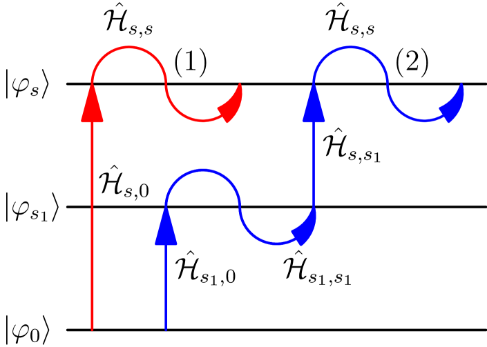
where $\hat{\mathcal{G}}_{0}$ can also be added as an identity operator $\hat{{I}}_{2p}$ with $\hat{{I}}_{2p}|\varphi_{0}\rangle=|\varphi_{0}\rangle$. For example, the operators $\hat{\mathcal{G}}_{1,2,3}(\varepsilon)$ are approximately given in Appendix B. Therefore, the projected state $|\varphi_{0}\rangle$ with a map, which a series of operators $\hat{\mathcal{G}}_{s}(\varepsilon)$ function as, covers the three-phase state $|\varphi\rangle$ completely and accurately. Equation (73) mathematically describes one physical understanding that for the states in the manifold $\mathcal{M}_{0}$ photons persisting in all of the excited levels come from the ground level via all possible PTPs as illustrated in Fig. 3 due to the perturbations of the inductance-free flux-qubit.

Substituting $|\varphi_{s}\rangle$ in Eq. (62) with the aid of Eq. (73), we have an eigen-like problem

$$\tilde{H}(\varepsilon)|\varphi_{0}\rangle=\varepsilon|\varphi_{0}\rangle,$$ (74)

where the pseudo-Hamiltonian $\tilde{H}(\varepsilon)$ is defined as

$$\tilde{H}(\varepsilon)=\hat{H}_{0,0}+\sum_{s>0}\hat{H}_{0,s}\hat{\mathcal{G}}_{s}(\varepsilon).$$ (75)

In the definition of $\tilde{H}(\varepsilon)$, all of the terms in the latter sum can be described in a general form $\hat{H}_{0,s}\hat{\mathcal{H}}_{s,s}^{i}(\varepsilon)\hat{\mathcal{H}}_{s,s_{1}}\hat{\mathcal{H}}_{s_{1},s_{1}}^{i_{1}}(\varepsilon)\hat{\mathcal{H}}_{s_{1},s_{2}}\cdots\hat{\mathcal{H}}_{s_{n-1},s_{n-1}}^{i_{n-1}}(\varepsilon)\hat{\mathcal{H}}_{s_{n-1},0}$ which can be interpreted in the terms of the photon-assisted transitions as that the LC photons spread to one specific excited level such as the $s$th one from the ground level through an arbitrary PTP (the role $\hat{\mathcal{G}}_{s}(\varepsilon)$ plays) and then return back ( an operator $\hat{H}_{0,s}$ closes the whole PTP). Therefore, the PTPs introduced by the operator $\tilde{H}(\varepsilon)$ are not only linked but also closed, starting from and ending with the ground level. It should be emphasized that a one-to-one correspondence is established between the terms in this sum and the closed photon transition paths(CPTP). Putting aside the details of the CPTPs in this section, one idea can be accepted that the longer path the photons travel along, the weaker effects are brought. Based on the BW expansion, the above derivations do not lose any accuracy thanks to the formal substitutions we utilize. Yet, as drawbacks, to make the whole solution available, we still need to deal with the infinite terms included in $\tilde{H}(\varepsilon)$ and its dependence on the eigenenergy $\varepsilon$ which is actually unknown before we successfully solve the problem.

One common solution for these two problems is to employ the standard RS perturbation method, which utilizes the expansions of $\varepsilon$ and $|\varphi_{0}\rangle$ in Eqs. (53) and (54), respectively, and all possible results can be achieved by checking terms on the same order of $\beta$ in Eqs. (73) and (74). This approach mixes up the BW and RS perturbation methods and benefits at least on two aspects due to a fact that perturbation effects of different strengths are able to coexist in one photon-transition matrix element which we can manipulate in a more physical manner. One is that instead of the step-by-step style we directly expand Eq. (74) on a specific order of $\beta^{1/4}$ and, consequently, achieve a series of equations including all of the cases below this order. In this context, our method now acts as an improved wrapper for the order analysis utilized by Ref. Alec2005, , and the difference is that we use the projections before the order comparisons while they prefer that the latter one goes first. The other is the convenience that we can more easily predict characteristics of the perturbation results. For example, without the emphasis on $s\hbar\omega_{LC}$ and the consequential result Eq. (73), it is not obvious in the previous paper that the projected states on the excited levels can be derived from $|\varphi_{0}\rangle$, although the term $s\hbar\omega_{LC}|\varphi_{s}^{(k+2)}\rangle$ in the expansion of Eq. (63) on $O(\beta^{k/4})$ with $k$ being an integer gives a hint in the RS perturbation method. To avoid that $\varepsilon$ and $|\varphi\rangle$ should be obtained in pair step by step in this method, we introduce a better one where the effective quantum states for the system are able to share a unique set of effective operators such as the effective Hamiltonian and the loop current operator.

IV.3 Effective Hamiltonian

Figure 4: (Color online) CPTPs of different types. The last steps of those CPTPs do not denote the $\hat{\mathcal{H}}_{0,s}$-like operators but the $\hat{{H}}_{0,s}$-like ones.

Table 1: For typical CPTPs labeled in Fig. 4, their corresponding operators and the orders of their dominant terms on $\beta$ are listed. The CPTPs P1, P3 and P8 denote the cases of the direct connection type for the first, second and third excited levels, respectively. By checking the orders, it is found that P1 is stronger than any CPTP involving the first excited level such as P2, P5, P6 and P7. The photon energy denominator in the self-transition operator ${\hat{\mathcal{H}}_{1,1}}(\varepsilon)$ yields that P2 is weaker than P1.

Label	Operator	Order
P1	$\hat{\mathcal{P}}_{1}=\hat{H}_{0,1}{\hat{\mathcal{H}}_{1,0}}$	$\beta^{1}$
P2	$\hat{\mathcal{P}}_{2}=\hat{H}_{0,1}{\hat{\mathcal{H}}_{1,1}}(\varepsilon){\hat{\mathcal{H}}_{1,0}}$	$\beta^{3/2}$
P3	$\hat{\mathcal{P}}_{3}=\hat{H}_{0,2}{\hat{\mathcal{H}}_{2,0}}$	$\beta^{3/2}$
P4	$\hat{\mathcal{P}}_{4}=\hat{H}_{0,2}{\hat{\mathcal{H}}_{2,2}}(\varepsilon){\hat{\mathcal{H}}_{2,0}}$	$\beta^{2}$
P5 and P6	$\hat{\mathcal{P}}_{5}=\hat{\mathcal{P}}_{6}^{{\dagger}}=\hat{H}_{0,1}{\hat{\mathcal{H}}_{1,2}}{\hat{\mathcal{H}}_{2,0}}$	$\beta^{2}$
P7	$\hat{\mathcal{P}}_{7}=\hat{H}_{0,1}{\hat{\mathcal{H}}_{1,2}}{\hat{\mathcal{H}}_{2,1}}{\hat{\mathcal{H}}_{1,0}}$	$\beta^{5/2}$
P8	$\hat{\mathcal{P}}_{8}=\hat{H}_{0,3}{\hat{\mathcal{H}}_{3,0}}$	$\beta^{2}$

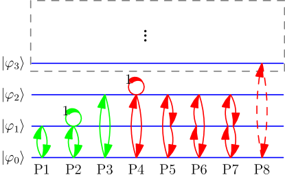
The photon transition path concept leads to an easier understanding on $\tilde{H}(\varepsilon)$. Let us expand $\tilde{H}(\varepsilon)$ to order $\beta^{3/2}$ with the aid of Fig. 4 and Table 1. To begin with, like $\hat{H}_{s,s_{1}}$ in Eq. (61), each CPTP operator in $\tilde{H}(\varepsilon)$ holds its own identical dominant term, the order of which facilitates comparing its relative strength with others. According to the order analysis ( see Appendix A for some details ), all of the CPTPs involving the third or higher excited levels, among which the one P8 $\hat{\mathcal{P}}_{8}=\hat{H}_{0,3}{\hat{\mathcal{H}}_{3,0}}$ provides the maximum correction on $O(\beta^{2})$, can be dropped as well as the infinite weak ones bound in the three lowest levels, i.e., from P4 to P7, and a sum of the remaining three ones P1, P2 and P3 yields one approximate pseudo-Hamiltonian $\tilde{H}^{(3/2)}(\varepsilon)$ as

$$\tilde{H}^{(3/2)}(\varepsilon) = \hat{H}_{0,0}-\hat{H}_{0,1}\frac{\hat{H}_{1,0}}{\hbar\omega_{LC}}+\hat{H}_{0,1}\frac{(\hat{H}_{1,1}-\varepsilon)\hat{H}_{1,0}}{(\hbar\omega_{LC})^{2}}-\hat{H}_{0,2}\frac{\hat{H}_{2,0}}{2\hbar\omega_{LC}},$$ (76)

where its superscript “$(3/2)$” annotates that it is expanded on $O(\beta^{3/2})$ and partial higher order terms are also included. The equation $\tilde{H}^{(3/2)}(\varepsilon)|\varphi_{0}\rangle=\varepsilon|\varphi_{0}\rangle$ becomes a generalized eigen-problem

$$\tilde{H}^{(3/2)}_{L}|\varphi_{0}\rangle = \varepsilon\hat{R}|\varphi_{0}\rangle+O(\beta^{7/4}),$$ (77)

where

$$\tilde{H}^{(3/2)}_{L} = \hat{H}_{0,0}-\frac{\hat{H}_{0,1}\hat{H}_{1,0}}{\hbar\omega_{LC}}+\frac{\hat{H}_{0,1}\hat{H}_{1,1}\hat{H}_{1,0}}{(\hbar\omega_{LC})^{2}}-\frac{\hat{H}_{0,2}\hat{H}_{2,0}}{2\hbar\omega_{LC}},$$ (78)

$$\hat{R} = 1+\frac{\hat{H}_{0,1}\hat{H}_{1,0}}{(\hbar\omega_{LC})^{2}}.$$ (79)

Although Eq. (77) can be solved (see Appendix C for details), an alternative but more general way to eliminate the $\varepsilon$-dependence is to substitute $\tilde{H}(\varepsilon)$ for $\varepsilon$ in the perturbation terms of $\tilde{H}(\varepsilon)$. For instance, to deal with the term $-\frac{\hat{H}_{0,1}\varepsilon\hat{H}_{1,0}}{(\hbar\omega_{LC})^{2}}|\varphi_{0}\rangle$ , we can multiply $\varepsilon$, a constant number commuting with any operator, and $|\varphi_{0}\rangle$ first of all, and then replace $\varepsilon|\varphi_{0}\rangle$ with $\tilde{H}(\varepsilon)|\varphi_{0}\rangle$ as follows,

$$-\frac{\hat{H}_{0,1}\varepsilon\hat{H}_{1,0}}{(\hbar\omega_{LC})^{2}}|\varphi_{0}\rangle=-\frac{\hat{H}_{0,1}\hat{H}_{1,0}}{(\hbar\omega_{LC})^{2}}\tilde{H}(\varepsilon)|\varphi_{0}\rangle{=}-\frac{\hat{H}_{0,1}\hat{H}_{1,0}}{(\hbar\omega_{LC})^{2}}\hat{H}_{0,0}|\varphi_{0}\rangle+{O}(\beta^{7/4}),$$ (80)

where only $\hat{H}_{0,0}$ in $\tilde{H}(\varepsilon)$ is kept in the final expansion. Therefore, $\tilde{H}^{(3/2)}(\varepsilon)$ gets rid of its $\varepsilon$-dependence but changes to a non-Hermitian effective operator $\tilde{H}^{(3/2)}_{nh}$ as

$$\tilde{H}^{(3/2)}_{nh} = \tilde{H}^{(3/2)}_{L}-\frac{\hat{H}_{0,1}\hat{H}_{1,0}\hat{H}_{0,0}}{(\hbar\omega_{LC})^{2}}.$$ (81)

Generally, because this kind of substitutions can continue to increase the orders of $\beta$ of the remaining $\varepsilon$-dependent terms in $\tilde{H}(\varepsilon)$ until the result does not depend on $\varepsilon$ on the order we want, this approach, namely the $\varepsilon$-$\tilde{H}(\varepsilon)$ substitution, can formally achieve an accurate and $\varepsilon$-independent operator $\tilde{H}_{nh}$ which, however, loses its Hermiticity completely just like $\tilde{H}^{(3/2)}_{nh}$, its expansion on $O(\beta^{3/2})$. As discussed in the previous papersKlein73 ; Duan2001 ; Cherny2004 , the non-Hermiticity comes with that $|\varphi_{0}\rangle$ is not a good effective state candidate in the equation

$$\tilde{H}_{nh}|\varphi_{0}\rangle = \varepsilon|\varphi_{0}\rangle.$$ (82)

If we introduce another eigenstate $|\psi\rangle$ with its eigenenergy being $\varepsilon_{\psi}$ and $\varepsilon$ is rewritten as $\varepsilon_{\varphi}$ for the sake of symmetry, there exists an identity overlap problem as

$$\langle\psi_{0}|\varphi_{0}\rangle\neq\delta_{\psi,\varphi},$$ (83)

which is also indicated by the generalized eigen-problem Eq. (77). In fact, defining an operator vector $\vec{\mathcal{G}}=[\hat{\mathcal{G}}_{0},\hat{\mathcal{G}}_{1},\cdots]^{T}$ (Analogously, one can also drop the $\varepsilon$-dependence of the operators $\hat{\mathcal{G}}_{1}(\varepsilon)$, $\hat{\mathcal{G}}_{2}(\varepsilon)$, $\cdots$ as we do in Appendix B) with its norm being

$$\hat{\mathcal{G}}_{||}=\hat{\mathcal{G}}^{{\dagger}}_{||}=\left(\sum_{s}\hat{\mathcal{G}}_{s}^{{\dagger}}\hat{\mathcal{G}}_{s}\right)^{\frac{1}{2}},$$ (84)

it is found that the orthogonality of the three-phase states $\langle\psi|\varphi\rangle=\delta_{\psi,\varphi}$ in the manifold $\mathcal{M}_{0}$ can be expressed by the components $\hat{\mathcal{G}}_{||}|\psi_{0}\rangle$ and $\hat{\mathcal{G}}_{||}|\varphi_{0}\rangle$ as

$$\delta_{\psi,\varphi} = \langle\psi_{0}|\hat{\mathcal{G}}_{||}^{\dagger}\hat{\mathcal{G}}_{||}|\varphi_{0}\rangle.$$ (85)

Let us construct a new equation from Eq. (82) as

$$\tilde{H}_{eff}|\varphi_{eff}\rangle = \varepsilon|\varphi_{eff}\rangle$$ (86)

with the two-phase effective state $|\varphi_{eff}\rangle$ being

$$|\varphi_{eff}\rangle=\hat{\mathcal{G}}_{||}|\varphi_{0}\rangle$$ (87)

and the operator $\tilde{H}_{eff}$ being

$$\tilde{H}_{eff}=\hat{\mathcal{G}}_{||}\tilde{H}_{nh}\hat{\mathcal{G}}_{||}^{-1}.$$ (88)

According to Eq. (85), we have restored the orthogonality of the effective states. Fortunately, the operator $\tilde{H}_{eff}$ is also Hermitian (see Appendix D for the proofs). Therefore, the effective Hamiltonian $\tilde{H}_{eff}$ with $|\varphi_{eff}\rangle$ can describe the manifold $\mathcal{M}_{0}$ of the three-phase system accurately in a compact two-phase subspace.

We here give some comments on the availabilities of this method via a comparison to the UT method. According to the above definitions, it is not difficult to obtain

$$\hat{H}_{tr}\vec{\mathcal{G}}\hat{\mathcal{G}}_{||}^{-1}|\varphi_{eff}\rangle=\vec{\mathcal{G}}\hat{\mathcal{G}}_{||}^{-1}\tilde{H}_{eff}|\varphi_{eff}\rangle.$$ (89)

Since the state $|\varphi_{eff}\rangle$ is arbitrary and the vector $\vec{\mathcal{G}}\hat{\mathcal{G}}_{||}^{-1}$ is explicitly unitary, our method exactly focuses on the manifold $\mathcal{M}_{0}$ and presents a formal solution on its corresponding eigenvector belonging to the transformation $\hat{T}$ in the UT method. So $\tilde{H}_{0}$ and $|\tilde{\varphi}_{0}\rangle$ in the UT method are equivalently $\tilde{H}_{eff}$ and $|\varphi_{eff}\rangle$ here, respectively. The UT method achieves the expanded operator $\hat{S}$ instead of $\hat{T}=e^{i\hat{S}}$, suggesting that it may work more efficiently when the order becomes higher. The PTP approach, however, gives clear pictures to handle the expansions on lower orders and also successfully predicts the properties of this problem. For instance, since the well-known optical selection rules forbid the photons to take odd times of creating and annihilating processes to go back to the same level and since the corresponding operators $\hat{a}^{{\dagger}}$ and $\hat{a}$ are always associated with a factor proportional to $\beta^{1/4}$, it is found that there only exist non-zero terms on the orders of $\beta^{1/4}$ to even powers in $\tilde{H}_{eff}$, some hints on which have been given by the orders of the dominant terms in the CPTPs shown in Table 1. See Appendix A for more details. So with an arbitrary integer $r$, we have $\tilde{H}_{eff}$ in the expansion to order $\beta^{r/2}$ as

$$\tilde{H}_{eff}^{(r/2)} = \sum_{k=0}^{r}\tilde{H}_{eff}|_{\beta^{k/2}}+O(\beta^{\frac{r+1}{2}}),$$ (90)

where the operator $\tilde{H}_{eff}|_{\beta^{k/2}}$ is in proportion to ${\beta^{k/2}}$. In our method, the effective Hamiltonian $\tilde{H}_{eff}^{(r/2)}$ may selectively keep some higher order terms for easier calculations and denotations, but the non-trivial terms $\tilde{H}_{eff}|_{\beta^{k/2}}$ for $k=0,1,\cdots,r$ are uniquely determined and it still bears an error on $\beta^{{(r+1)}/{2}}$. Consequentially, one can have the eigen-problem with improved conditions as

$$\varepsilon^{(2k+1)}\equiv 0,$$ (91)

$$|\varphi_{0}^{(2k+1)}\rangle\equiv 0,$$ (92)

where $k$ is an integer, and both $\varepsilon^{(k)}$ and $|\varphi_{0}^{(k)}\rangle$ are in proportion to $\beta^{k/4}$ defined in Eqs. (53) and (54), respectively.

Back to Eq. (81), with the method provided by Eq. (86) and the expansion of $\hat{\mathcal{G}}_{||}$ on $O(\beta^{3/2})$ being

$$\hat{\mathcal{G}}_{||}^{(3/2)} = 1+\frac{\hat{H}_{0,1}\hat{H}_{1,0}}{2(\hbar\omega_{LC})^{2}},$$ (93)

we have the effective Hamiltonian $\tilde{H}_{eff}^{(3/2)}=\left(\tilde{H}_{eff}^{(3/2)}\right)^{{\dagger}}$ as

$$\tilde{H}^{(3/2)}_{eff} = \hat{H}_{0,0}+\tilde{H}_{0,1,0}+\tilde{H}_{0,2,0}+\tilde{H}^{(3/2)}_{3},$$ (94)

where

$$\tilde{H}_{0,1,0} = -\frac{\hat{H}_{0,1}\hat{H}_{1,0}}{\hbar\omega_{LC}},$$ (95)

$$\tilde{H}_{0,2,0} = -\frac{\hat{H}_{0,2}\hat{H}_{2,0}}{2\hbar\omega_{LC}},$$ (96)

$$\tilde{H}^{(3/2)}_{3} = \frac{\hat{H}_{0,1}\hat{H}_{1,1}\hat{H}_{1,0}}{(\hbar\omega_{LC})^{2}}-\frac{1}{2}\frac{\hat{H}_{0,1}\hat{H}_{1,0}\hat{H}_{0,0}+\hat{H}_{0,0}\hat{H}_{0,1}\hat{H}_{1,0}}{(\hbar\omega_{LC})^{2}}.$$ (97)

Let us scrutinize the terms in the effective Hamiltonian $\tilde{H}_{eff}^{(3/2)}$. The first term $\hat{H}_{0,0}$=$\langle\Omega_{0}|\hat{H}_{tr}|\Omega_{0}\rangle$ originates from the projection on the ground level of the oscillator. Besides including the inductance-free two-phase Hamiltonian $\hat{H}_{0}$, it also takes into account the vacuum fluctuations of the oscillator, both of which in total read

$$\hat{H}_{0,0} = \frac{1}{2}{\hat{\mathbf{Q}}_{\theta}^{T}\mathbf{C}_{2p}^{-1}\hat{\mathbf{Q}}_{\theta}}-\sum_{k=1}^{3}e^{-\gamma_{k}^{2}/2}E_{Jk}\cos\theta_{k},$$ (98)

where $\gamma_{k}$ is a dimensionless factor as

$$\gamma_{k} = \frac{\alpha_{ser}}{\alpha_{k}}\sqrt[4]{\frac{2\beta}{g\alpha_{ser}}},k=1,2,3$$ (99)

with a ratio parameter

$$g=\frac{E_{J0}}{E_{C0}}=\frac{\Phi_{0}I_{C0}C_{0}}{\pi e^{2}}$$ (100)

showing a typical Josephson energy $E_{J0}$ compared to the charging energy $E_{C0}$. Because the sinusoidal potential of each junction is equal to zero on average, the vacuum fluctuations equivalently flush the junction energy $E_{Jk}$ into a weaker one $E^{\prime}_{Jk}$ as

$$E^{\prime}_{Jk} = e^{-\gamma_{k}^{2}/2}E_{Jk},k=1,2,3,$$ (101)

which indicates that the effective size of the $k$th junction is reduced by a factor $e^{-\gamma_{k}^{2}/2}$ which gives a correction maximized on $O(\beta^{1/2})$.

The non-positive term $\tilde{H}_{0,1,0}$ providing main effects on $O(\beta)$ relates to the interactions between the two lowest levels of the oscillator. The states in the manifold $\mathcal{M}_{0}$ with $\varepsilon\ll\hbar\omega_{LC}$ hardly afford one high-frequency LC photon so that the first excited level of the oscillator is almost empty due to the ensuing energy punishment. Since the state occupying the ground level can spread into the first excited level and also accept its feedbacks due to the bidirectional transitions $\hat{H}_{0,1}$ and $\hat{H}_{1,0}$ between those two levels brought by the two-phase flux qubit system, the almost empty excited level acts as a “mirror” for the ground one, which endows a correction $\tilde{H}_{0,1,0}$ to minimize the eigenenergy of the eigenstates. According to Appendix B, we have

$$\tilde{H}_{0,1,0} = -\frac{1}{2}L\left(\tilde{I}_{\phi}^{(2)}\right)^{2},$$ (102)

where the $\beta$-independent current operator

$$\tilde{I}_{\phi}^{(0)} = C_{ser}\sum_{k=1}^{3}\frac{I_{Ck}}{C_{k}}\sin\theta_{k}$$ (103)

resembles $I_{loop}(t)$ in Eq. (8) with $\phi_{1}$, $\phi_{2}$ and $\phi_{3}$ being replaced by the effective phase variables $\theta_{1}$, $\theta_{2}$ and $\theta_{3}$, respectively, and dominates in

$$\tilde{I}_{\phi}^{(2)} = C_{ser}\sum_{k=1}^{3}\frac{e^{-\gamma_{k}^{2}/2}I_{Ck}}{C_{k}}\sin\theta_{k},$$ (104)

which equivalently keeps the critical current of the $k$th junction modified by a fluctuation factor $e^{-\gamma_{k}^{2}/2}$ like the case of $E^{\prime}_{Jk}$. It is worth noting that the coupling $\hat{V}_{1}\hat{\phi}=\frac{\Phi_{0}\hat{\phi}}{2\pi}\tilde{I}_{\phi}^{(0)}$ in $\hat{H}_{int}$ interestingly renders $\tilde{I}_{\phi}^{(0)}$ and also presents the dominant terms in $\hat{H}_{0,1}$ and $\hat{H}_{1,0}$. To emphasize it, we assume that those two subsystems couple with each other only by $\hat{V}_{1}\hat{\phi}$ and have the Hamiltonian

$$\hat{H}_{tr,\phi} = \hat{H}_{0}-\frac{1}{2}L\left(\tilde{I}_{\phi}^{(0)}\right)^{2}+\hat{D}_{\hat{a}^{\dagger}\hat{a}},$$ (105)

where the operator

$$\hat{D}_{\hat{a}^{\dagger}\hat{a}} = \frac{\hat{Q}^{2}_{\phi}}{2C_{ser}}+\frac{1}{2L}\left(\frac{\Phi_{0}}{2\pi}\hat{\phi}+L\tilde{I}_{\phi}^{(0)}\right)^{2}$$ (106)

indicates an LC-oscillator with an additional flux displacement $-L\tilde{I}_{\phi}^{(0)}$. In a semi-classical picture, the above formula suggests that the average value of the current in the loop inductance is expected to be $\tilde{I}_{\phi}^{(0)}$ as a function of the slow junction phases instead of a real zero value when $L\rightarrow 0$, so $\tilde{I}_{\phi}^{(0)}$ can be understood as the loop current produced by the junctions which drives the inductance to generate an additional small flux. As a result of that the slow-varying-function biased LC-oscillator does not change its own eigenenergy significantly, the inductive energy $-\frac{1}{2}L\left(\tilde{I}_{\phi}^{(0)}\right)^{2}$ on $O(\beta)$ is added as one perturbation correction to the effective two-phase Hamiltonian, which can be explained as that the flux generated by $\tilde{I}_{\phi}^{(0)}$ in the inductance also affects the junctions themselves. Intuitively, this self-bias effect persistently lowers the potential on any point which keeps a non-zero current and always opposes the current direction switching. In the quantum regime, this kind of understanding is still supported by the facts that the estimation $\langle\varphi|\hat{D}_{\hat{a}^{\dagger}\hat{a}}|\varphi\rangle=\frac{1}{2}\hbar\omega_{LC}+O(\beta^{3/2})$ provides no effect on $O(\beta)$ and that the inductive energy correction dominates in $\tilde{H}_{0,1,0}$. Furthermore, a rigorous analysis in the next section also confirms that $\tilde{I}_{\phi}^{(0)}$ is the loop current operator for the inductance-free flux qubit.

The term $\tilde{H}_{0,2,0}$ shows the direct interactions between the ground and the second excited levels of the LC-oscillator via two-photon transitions. Photons travel forth and back via the bidirectional transitions $\hat{H}_{0,2}$ and $\hat{H}_{2,0}$, resulting in a non-positive operator

$$\frac{\tilde{H}_{0,2,0}}{E_{J0}} = -\frac{1}{4}\sqrt{\frac{\alpha_{ser}^{7}\beta^{3}}{2g}}\left(\sum_{k=1}^{3}\frac{e^{-\frac{\gamma^{2}_{k}}{2}}}{\alpha_{k}}\cos\theta_{k}\right)^{2},$$ (107)

according to Appendix B. Its main effects are on $O(\beta^{3/2})$ contributed by the coupling $\hat{V}_{2}\hat{\phi}^{2}\neq 0$ in $\hat{H}_{int}$.

Finally, the last term $\tilde{H}^{(3/2)}_{3}$ corresponds to the CPTP operator $\hat{\mathcal{P}}_{2}=\hat{H}_{0,1}{\hat{\mathcal{H}}_{1,1}}(\varepsilon){\hat{\mathcal{H}}_{1,0}}$ which includes the self-transition ${\hat{\mathcal{H}}_{1,1}}(\varepsilon)$ of the first excited level. Since the capacitive energy part $\frac{1}{2}{\hat{\mathbf{Q}}_{\theta}^{T}\mathbf{C}_{2p}^{-1}\hat{\mathbf{Q}}_{\theta}}$ of the unperturbed Hamiltonian $\hat{H}_{0}$ does not commute with $\hat{H}_{1,0}$ and $\hat{H}_{0,1}$ which turn out as functions of the effective phase variables $\hat{\theta}_{1}$ and $\hat{\theta}_{2}$, in the effective phase representation ($\theta_{1}$,$\theta_{2}$) with

$$\left[\left[\frac{\partial}{\partial\theta_{s}}\frac{\partial}{\partial\theta_{t}},f\right],f\right] = 2\frac{\partial{f}}{\partial\theta_{s}}\frac{\partial{f}}{\partial\theta_{t}},\text{for }s,t=1,2,$$ (108)

simplifying the right hand side of Eq. (97) yields $\tilde{H}^{(3/2)}_{3}$ in a symmetric form for the three junctions as

$$\tilde{H}^{(3/2)}_{3} = -\frac{L}{8\hbar\omega_{LC}}\left[\left[{\hat{\mathbf{Q}}_{\theta}^{T}\mathbf{C}_{2p}^{-1}\hat{\mathbf{Q}}_{\theta}},\tilde{I}_{\phi}^{(0)}\right],\tilde{I}_{\phi}^{(0)}\right]+O(\beta^{2}),$$ (109)

$$\tilde{H}^{(3/2)}_{3}/f = \sum^{3}_{k=1}\alpha_{k}\sum^{3}_{k=1}\cos^{2}\theta_{k}-\sum^{3}_{k=1}\alpha_{k}\cos^{2}\theta_{k}-2\prod^{3}_{k=1}\cos\theta_{k}\sum^{3}_{k=1}\frac{\alpha_{k}}{\cos\theta_{k}}+O(\beta^{2}),$$ (110)

where

$$f = {\sqrt{\frac{\alpha_{ser}^{7}\beta^{3}}{2g\prod^{3}_{k=1}\alpha_{k}^{2}}}}E_{J0}.$$ (111)

Therefore, the effective Hamiltonian $\tilde{H}^{(3/2)}_{eff}$ has taken account of four corrections of different types to the unperturbed one $\hat{H}_{0}$. Its complicated expression indicates that treating the LC-oscillator as a three-level system does not stand as an easy task on the derivations and analysis. First of all, unlike common perturbation situations where two subsystems couple with each other via a weak linear interaction, the Josephson junctions exhibiting as nonlinear inductances keep the interaction $\hat{H}_{int}$ in Eq.(51) split into the couplings of different strengths. For instance, among the effective corrections in proportion to $\beta^{3/2}$, $\hat{V}_{6}\hat{\phi}^{6}$ donates one as $\hat{V}_{6}\langle\Omega_{0}|\hat{\phi}^{6}|\Omega_{0}\rangle$ in $\hat{H}_{0,0}$, and $\hat{V}_{3}\hat{\phi}^{3}$ as $-{(\hbar\omega_{LC})}^{-1}{\hat{V}_{3}\langle\Omega_{0}|\hat{\phi}^{3}|\Omega_{1}\rangle\hat{V}_{1}\langle\Omega_{1}|\hat{\phi}|\Omega_{0}\rangle}$ in $\tilde{H}_{0,1,0}$. This kind of terms inside the photon-transition operators $\hat{H}_{s,s_{1}}$ have been automatically included in our results while the step-by-step method should explicitly calculate them out. On the other hand, $\hat{V}_{2}\hat{\phi}^{2}$ turns on the direct connections between the second excited level and the ground one, thus straightforwardly imposing the influences of this excited level without the help of any other excited one; otherwise, only with $\hat{V}_{1}\hat{\phi}$ its maximum feedback decreases to the CPTP P7 $\hat{\mathcal{P}}_{7}=\hat{H}_{0,1}{\hat{\mathcal{H}}_{1,2}}{\hat{\mathcal{H}}_{2,1}}{\hat{\mathcal{H}}_{1,0}}$ in Table 1, the dominant term of which is on $O(\beta^{5/2})$. Thus our method also needs to accumulate suitable CPTPs one by one. Moreover, although being a part of the effective potential in $\tilde{H}_{eff}^{(3/2)}$, the operator $\tilde{H}^{(3/2)}_{3}$ involves one self-transition process and performs as a correction sensitive to the eigenenergy ( see the pseudo-Hamiltonian $\tilde{H}^{(3/2)}(\varepsilon)$ ). This feature is not good for the analysis of the experiments which often alter the energy level structure of the whole system by changing the external flux bias. After solving the eigen-problem of $\tilde{H}^{(3/2)}_{eff}$, although the eigenvalue $\tilde{\varepsilon}^{(3/2)}$ directly gives

$$\varepsilon=\tilde{\varepsilon}^{(3/2)}+O(\beta^{2}),$$ (112)

the effective state $|\varphi_{eff}^{(3/2)}\rangle$ should be preprocessed as

$$|\varphi_{0}\rangle = \left(1-\frac{\hat{H}_{0,1}\hat{H}_{1,0}}{2(\hbar\omega_{LC})^{2}}\right)|\varphi_{eff}^{(3/2)}\rangle+O(\beta^{2})$$ (113)

for further discussions. Even if the difficulties mentioned above are carefully handled, we should still cope with tens of terms related to $\alpha_{1,2,3}$, $\beta$ and $g$. Limited by the fabrication conditions and other factors, the loop inductance cannot be enlarged too much, and thus the $O(\beta^{3/2})$-effects appear essential in rare cases. Therefore, as a compromise between simplicity and accuracy, we choose one effective Hamiltonian on $O(\beta)$ rougher but optimal in this trade-off as

$$\tilde{H}^{(1)}_{eff} = \hat{H}_{0,0}-\frac{\hat{H}_{0,1}\hat{H}_{1,0}}{\hbar\omega_{LC}},$$ (114)

which bears an error on $O(\beta^{3/2})$. Dropping the terms in proportion to $\beta^{3/2}$ or higher orders of $\beta$ in Eq. (114) yields an effective potential

$$\tilde{V}_{eff}^{(1)} = -\sum_{k=1}^{3}\left(1-\sqrt{\frac{\alpha_{ser}^{3}}{2g\alpha_{k}^{4}}}\beta^{\frac{1}{2}}+{\frac{\alpha_{ser}^{3}}{4g\alpha_{k}^{4}}}\beta\right)E_{Jk}\cos\theta_{k}-\frac{1}{2}L\left(\tilde{I}_{\phi}^{(0)}\right)^{2}$$ (115)

identical to the one presented by Ref.Alec2005, . The corresponding normalized effective eigenstate $|\varphi_{eff}^{(1)}\rangle$ approximates $|\varphi_{0}\rangle$ on $O(\beta)$ as

$$|\varphi_{0}\rangle = |\varphi_{eff}^{(1)}\rangle+O(\beta^{3/2})$$ (116)

with the eigenenergy $\tilde{\varepsilon}^{(1)}$ being

$$\varepsilon=\tilde{\varepsilon}^{(1)}+O(\beta^{3/2}).$$ (117)

IV.4 Arbitrary effective operator

As mentioned above, the photon transition path method presents not only an accurate prediction on the eigenenergy by the effective Hamiltonian but also a full description of how an effective two-phase system is mapped to the three-phase one. Take an arbitrary three-phase operator $\hat{F}$ as an example. Assume that two arbitrary eigenstates $|\varphi\rangle$ and $|\psi\rangle$ in the manifold $\mathcal{M}_{0}$ go with their eigenenergy $\varepsilon_{\varphi}$ and $\varepsilon_{\psi}$, respectively, where $|\varphi\rangle$ may equate to $|\psi\rangle$. The expansions

$$\hat{F} = \sum_{m,n}|\Omega_{m}\rangle\hat{F}_{m,n}\langle\Omega_{n}|,$$ (118)

$$|\varphi\rangle = \sum_{s}\left(\hat{\mathcal{G}}_{s}|\varphi_{0}\rangle\right)|\Omega_{s}\rangle,$$ (119)

$$|\psi\rangle = \sum_{s}\left(\hat{\mathcal{G}}_{s}|\psi_{0}\rangle\right)|\Omega_{s}\rangle.$$ (120)

yield

$$\langle\psi|\hat{F}|\varphi\rangle = \langle\psi_{0}|\left(\sum_{m,n}\hat{\mathcal{G}}_{m}^{\dagger}\hat{F}_{m,n}\hat{\mathcal{G}}_{n}\right)|\varphi_{0}\rangle$$

$$= \langle\psi_{eff}|\tilde{F}_{eff}|\varphi_{eff}\rangle,$$

where we define the effective operator for $\hat{F}$ as

$$\tilde{F}_{eff} = \sum_{m,n}\left(\hat{\mathcal{G}}_{m}\hat{\mathcal{G}}_{||}^{-1}\right)^{\dagger}\hat{F}_{m,n}\hat{\mathcal{G}}_{n}\hat{\mathcal{G}}_{||}^{-1}.$$ (122)

The two-phase effective operator $\tilde{F}_{eff}$ depends not only on $\hat{F}_{m,n}$, for example, which may obey the optical selection rules, but also on $\hat{\mathcal{G}}_{m}$, $\hat{\mathcal{G}}_{n}$ and $\hat{\mathcal{G}}_{||}^{-1}$ which portray all of the projected components of the eigenstates in the three-phase system. Especially, for $\hat{F}$ as the three-phase identity operator $\hat{I}$, one can have

$$\tilde{I}_{eff} = \sum_{n}\left(\hat{\mathcal{G}}_{n}\hat{\mathcal{G}}_{||}^{-1}\right)^{\dagger}\hat{\mathcal{G}}_{n}\hat{\mathcal{G}}_{||}^{-1}=\hat{I}_{2p},$$ (123)

where $\hat{I}_{2p}$ is the identity operator for the effective two-phase subspace; for $\hat{F}=\hat{H}_{tr}$, with Eq. (89) we have a self-consistent result as

$$\left(\hat{H}_{tr}\right)_{eff} = \left(\vec{\mathcal{G}}\hat{\mathcal{G}}_{||}^{-1}\right)^{H}\hat{H}_{tr}\vec{\mathcal{G}}\hat{\mathcal{G}}_{||}^{-1}=\tilde{H}_{eff}.$$ (124)

V effective current operator

In the three-phase system, the current operator can be achieved in different ways: on the one hand, the definition of the loop inductance $L$ yields that

$$\hat{I}_{\phi}=-\frac{\hat{\Phi}_{L}}{L}=-\frac{\Phi_{0}}{2\pi L}\hat{\phi};$$ (125)

on the other hand, according to Kirchhoff’s current law, the series current flowing towards the $k$th junction(for $k=1$, 2 and 3) can be expressed as a sum of its Josephson supercurrent $I_{Ck}\sin\hat{\phi}_{k}$ and the one through the capacitor $C_{k}$, which due to the time variation of the charge $\hat{Q}_{k}$ is provided by the Heisenberg equation

$$\dot{Q}_{k} = \left[\hat{H}_{tr},i\hat{Q}_{k}/\hbar\right]=\hat{I}_{\phi}-I_{Ck}\sin\hat{\phi}_{k}.$$ (126)

One can simply find that the series current operator of the loop possesses a unique form $\hat{I}_{\phi}$.

The virtual work principle, besides the direct derivation above, also suggests some reasonable forms as

$$\hat{I}_{\partial\Phi_{X}} = \frac{\partial\hat{V}_{tr}}{\partial\Phi_{X}},$$ (127)

where $\hat{V}_{tr}$ is the potential term of $\hat{H}_{tr}$, because for the eigenstate $|\varphi\rangle$ we have

$$\langle\varphi|\hat{I}_{\partial\Phi_{X}}|\varphi\rangle=\langle\varphi|\frac{\partial\hat{H}_{tr}}{\partial\Phi_{X}}|\varphi\rangle=\frac{\partial{\varepsilon}_{\varphi}}{\partial\Phi_{X}}.$$ (128)

However, since the translations such as the one in Eq. (28) can alter the dependence of $\hat{V}_{tr}$ on $\Phi_{X}$, lots of current operators such as $\hat{I}_{\phi}$, the DC current operators $I_{Ck}\sin\hat{\phi}_{k}$ for k=1,2 and 3, etc, are possible candidates in this approach, which all provide the same diagonal matrix elements $\langle\varphi|\hat{I}_{\partial\Phi_{X}}|\varphi\rangle$ equal to $\partial{\varepsilon_{\varphi}}/\partial{\Phi_{X}}$. Unfortunately, this method cannot inform us which one is proper for the non-diagonal elements.

With the current operator being ready for the three-phase system, one can expand it in the oscillator-subsystem as

$$\langle\Omega_{m}|\hat{I}_{\phi}|\Omega_{n}\rangle = -\sqrt[4]{\frac{\hbar^{2}}{4C_{ser}L^{3}}}\left(\sqrt{m}\delta_{m,n+1}+\sqrt{n}\delta_{m+1,n}\right).$$ (129)

With the effective theory shown in Eqs. (IV.4) and (122), it yields that

$$\langle\psi|\hat{I}_{\phi}|\varphi\rangle = -\sqrt[4]{\frac{\hbar^{2}}{4C_{ser}L^{3}}}\sum_{k\geq 1}\sqrt{k}\left(\langle\psi_{k}|\varphi_{k-1}\rangle+\langle\psi_{k-1}|\varphi_{k}\rangle\right)$$ (130)

and

$$\tilde{I}_{\phi} = -\sqrt[4]{\frac{\hbar^{2}}{4C_{ser}L^{3}}}\sum_{k\geq 1}\sqrt{k}\left(\hat{\mathcal{G}}_{||}^{-1}\right)^{\dagger}\left(\hat{\mathcal{G}}_{k}^{\dagger}\hat{\mathcal{G}}_{k-1}+\hat{\mathcal{G}}_{k-1}^{\dagger}\hat{\mathcal{G}}_{k}\right)\hat{\mathcal{G}}_{||}^{-1},$$ (131)

where the tilde symbol labels the effective operators.

Let us check the dependence of $\tilde{I}_{\phi}$ on the reduced inductance $\beta$. The dimensional factor $\sqrt[4]{\frac{\hbar^{2}}{4C_{ser}L^{3}}}$, belonging to $\hat{I}_{\phi}$ in proportion to $\beta^{-3/4}$ , indicates that this current operator $\hat{I}_{\phi}$ generally diverges with the loop size. For example, the state $|\varphi\rangle$ with $|\langle\varphi_{0}|\varphi_{1}\rangle|=\frac{1}{2}$ carries an infinite loop-current $\langle\varphi|\hat{I}_{\phi}|\varphi\rangle$ when $\beta\rightarrow 0$. Oppositely, the optical selection rules zero out any rule-breaking term regardless of the order of its scale factor on $\beta$, so a real dark state $|\varphi_{dark}\rangle$ in the manifold $\mathcal{M}_{0}^{(0)}$ where the excited levels of the LC-oscillator are entirely empty is forbidden to possess a current circulating in the loop due to $\langle\Omega_{0}|\hat{\phi}|\Omega_{0}\rangle=0$. As a result, with the dimensional factor the largest term $\frac{\hat{H}_{1,0}}{\hbar\omega_{LC}}$ among the small perturbations left in the sum in Eq. (131) provides an inductance-independent operator $\tilde{I}_{\phi}^{(0)}$, which has been written in Eq.(103) and confirms that the junctions determine the loop current when the inductance is small enough. One interesting thing is that the effective counterpart for the photon number operator $\hat{a}^{\dagger}\hat{a}$,

$$(\hat{a}^{\dagger}\hat{a})_{eff} = \frac{L\left(\tilde{I}_{\phi}^{(0)}\right)^{2}}{2\hbar\omega_{LC}}+O(\beta^{2}),$$ (132)

is mainly determined by the inductive energy $L\left(\tilde{I}_{\phi}^{(0)}\right)^{2}/2$ divided by one LC-photon energy $\hbar\omega_{LC}$. Thus the eigenstates in the manifold $\mathcal{M}_{0}$ actually look dim with the average photon number being much less than one, neither dark with no photon completely nor bright with one or more photons.

Expanding Eq. (131) to order $\beta$, we obtain the effective current operator $\tilde{I}_{\phi}^{(4)}$ as

$$\tilde{I}_{\phi}^{(4)} = -\sqrt[4]{\frac{\hbar^{2}}{4C_{ser}L^{3}}}\left(\hat{\mathcal{G}}_{1}+\sqrt{2}\hat{\mathcal{G}}_{2}^{{\dagger}}\hat{\mathcal{G}}_{1}+h.c.\right)_{O(\beta^{{7}/{4}})},$$ (133)

where the LC-oscillator is involved as a three-level system and the operators in the parentheses such as $\hat{\mathcal{G}}_{1}$ should be expanded on ${O(\beta^{{7}/{4}})}$ denoted by the subscript. It is clear that the large dimensional factor leads to deeper explorations on the $\hat{\mathcal{G}}$-operators: $\hat{\mathcal{G}}_{1}$ should be expanded at least on ${O(\beta^{{7}/{4}})}$ in $\tilde{I}_{\phi}^{(4)}$ but on ${O(\beta^{{3}/{4}})}$ in $\tilde{H}_{eff}^{(1)}$ and on ${O(\beta^{{5}/{4}})}$ in $\tilde{H}_{eff}^{(3/2)}$. According to the optical selection rules, it is found that $\tilde{I}_{\phi}^{(4)}$ suffers from an error on $O(\beta^{3/2})$ compared to $\tilde{I}_{\phi}$ as

$$\tilde{I}_{\phi} = \tilde{I}_{\phi}^{(4)}+{O(\beta^{3/2})}.$$ (134)

Although the direct expansion in Eq. (133) can be accomplished with the help of Appendix B, since our effective theory can cope with arbitrary three-phase operators, one can also achieve $\tilde{I}_{\phi}^{(4)}$ via applying the theory to its another definition on $O(\beta)$. For the sake of clarity, $I_{C0}$ is utilized as the current unit, $\hbar=1$ and $e=1/2$. We construct a current operator

$$\hat{I}_{con} = \alpha_{ser}\sum_{k=1}^{3}\sin\hat{\phi}_{k}$$

$$= \hat{I}_{\cos}-\hat{\mathcal{\eta}}_{\beta}\hat{I}_{\phi}+\hat{I}_{\sin},$$

where according to Eqs. (29) and (40) it has been divided into three components as

$$\hat{I}_{\cos} = \alpha_{ser}\sum_{k=1}^{3}\sin\hat{\theta}_{k}\cos\frac{\alpha_{ser}}{\alpha_{k}}\hat{\phi},$$ (136)

$$\hat{\mathcal{\eta}}_{\beta} = \alpha_{ser}^{2}\beta\sum_{k=1}^{3}\frac{\cos\hat{\theta}_{k}}{\alpha_{k}},$$ (137)

$$\hat{I}_{\sin} = \alpha_{ser}\sum_{k=1}^{3}\cos\hat{\theta}_{k}\sin\frac{\alpha_{ser}}{\alpha_{k}}\hat{\phi}+\hat{\mathcal{\eta}}_{\beta}\hat{I}_{\phi}$$

$$= \alpha_{ser}^{4}\beta^{3}\hat{I}_{\phi}^{3}\sum_{k=1}^{3}\frac{\cos\hat{\theta}_{k}}{6\alpha_{k}^{3}}+\cdots.$$

With the aid of Eq. (126), it is not difficult to achieve that

$$\dot{Q}_{\phi}=\left[\hat{H}_{tr},i\hat{Q}_{\phi}/\hbar\right]=\hat{I}_{\phi}-\hat{I}_{con},$$ (139)

which reads

$$\dot{Q}_{\phi} = \left(1+\hat{\mathcal{\eta}}_{\beta}\right)\hat{I}_{\phi}-\hat{I}_{\cos}-\hat{I}_{\sin}.$$ (140)

Applying $\left(1-\hat{\mathcal{\eta}}_{\beta}\right)\cdot$ to both sides of the above equation, we have

$$\hat{I}_{\phi} = \left(1-\hat{\mathcal{\eta}}_{\beta}\right)\left(\hat{I}_{\cos}+\hat{I}_{\sin}+\dot{Q}_{\phi}\right)+\hat{\mathcal{\eta}}_{\beta}^{2}\hat{I}_{\phi}.$$ (141)

Utilizing the definition in Eq. (122), one can find that the effective operators of the three-phase ones $\left(1-\hat{\mathcal{\eta}}_{\beta}\right)\hat{I}_{\sin}$, $\hat{\mathcal{\eta}}_{\beta}\dot{Q}_{\phi}=\hat{\mathcal{\eta}}_{\beta}\left(\hat{I}_{\phi}-\hat{I}_{con}\right)$ and $\hat{\mathcal{\eta}}_{\beta}^{2}\hat{I}_{\phi}$ equate to zero on $O(\beta)$, and, thus, it follows that

$$\tilde{I}_{\phi}^{(4)}=\tilde{I}_{\phi}^{(2)}-\hat{\mathcal{\eta}}_{\beta}\tilde{I}_{\phi}^{(2)}+\dot{Q}_{\phi}^{eff}+O(\beta^{3/2}),$$ (142)

where

$$\tilde{I}_{\phi}^{(2)} = \langle\Omega_{0}|\hat{I}_{\cos}|\Omega_{0}\rangle=\langle\Omega_{0}|\hat{I}_{con}|\Omega_{0}\rangle,$$ (143)

$$\dot{Q}_{\phi}^{eff} = \frac{\left[\hat{H}_{0},\left[\hat{H}_{0},\tilde{I}_{\phi}^{(2)}\right]\right]}{\left(\hbar\omega_{LC}\right)^{2}}+O(\beta^{3/2}).$$ (144)

Three kinds of effects are taken into account in the above formula for $\tilde{I}_{\phi}^{(4)}$. The first term $\tilde{I}_{\phi}^{(2)}$ consistent with its definition in Eq. (104) shows that the projections $\langle\Omega_{0}|\cos\left({\alpha_{ser}}{\alpha_{k}}^{-1}\hat{\phi}\right)|\Omega_{0}\rangle$ impose the vacuum fluctuation factors $e^{-\gamma_{k}^{2}/2}$ to the corresponding terms in $\tilde{I}_{\phi}^{(0)}$ for $k=1$,2 and 3. The second term $-\hat{\mathcal{\eta}}_{\beta}\tilde{I}_{\phi}^{(2)}$ is traced back to $-\hat{\mathcal{\eta}}_{\beta}\hat{I}_{\phi}$ in $\hat{I}_{con}$ as the result of the linear approximations ${\alpha_{k}}^{-1}{\alpha_{ser}}\hat{\phi}$ for $\sin\left({\alpha_{k}}^{-1}{\alpha_{ser}}\hat{\phi}\right)$. And the final term $\dot{Q}_{\phi}^{eff}$ represents a tiny current $\dot{Q}_{\phi}$ flowing through the series capacitance $C_{ser}$, which can also be obtained from the direct expansion in Eq. (133) or the solution presented by Appendix E. As a two-fold commutator, it correspondingly involves a self-transition process $\hat{\mathcal{H}}_{1,1}^{2}(\varepsilon)\hat{\mathcal{H}}_{1,0}$ occurring in the first excited level of the oscillator and, thus, explains why the self-transition processes are able to challenge the Hermiticity of the effective Hamiltonian. With the effective states $|\psi_{eff}^{(1)}\rangle$ and $|\varphi_{eff}^{(1)}\rangle$, the matrix element $\langle\psi_{eff}^{(1)}|\dot{Q}_{\phi}^{eff}|\varphi_{eff}^{(1)}\rangle$ can be calculated numerically as

$$\langle\psi_{eff}^{(1)}|\dot{Q}_{\phi}^{eff}|\varphi_{eff}^{(1)}\rangle=\left(\frac{\tilde{\varepsilon}^{(1)}_{\psi}-\tilde{\varepsilon}^{(1)}_{\varphi}}{\hbar\omega_{LC}}\right)^{2}\langle\psi_{eff}^{(1)}|\tilde{I}_{\phi}^{(2)}|\varphi_{eff}^{(1)}\rangle+O(\beta^{3/2}),$$ (145)

where $\tilde{\varepsilon}^{(1)}_{\psi}$ and $\tilde{\varepsilon}^{(1)}_{\varphi}$ being involved indicates that the self-transition effects distinguish the corresponding eigenstates by their different eigenenergy.

Now we have a short summary of several effective current operators in the effective theory. The operator $\tilde{I}_{\phi}^{(0)}$ defined in Eq. (103) as an effective current operator excluding any inductive effect acts as the loop current operator for the inductance-free flux qubit system. The operator $\tilde{I}_{\phi}^{(2)}$ defined in Eq. (104) appearing in the effective Hamiltonian $\tilde{H}_{eff}^{(1)}$ contains the vacuum fluctuation corrections while both $\tilde{I}_{\phi}^{(0)}$ and $\tilde{I}_{\phi}^{(2)}$ treat the oscillator as a two-level system. The third one $\tilde{I}_{\phi}^{(4)}$, costing more, can include the effects brought by the second excited level of the oscillator and, especially, possesses a term coming from a self-transition process which the effective Hamiltonians $\tilde{H}_{eff}^{(1)}$ and $\tilde{H}_{eff}^{(3/2)}$ do not have. Formally, the effective current operator $\tilde{I}_{\phi}$ like $\tilde{H}_{eff}$ can be truncated on arbitrary orders. However, for the next step, to achieve the fourth one $\tilde{I}_{\phi}^{(6)}$ accurate on $O(\beta^{3/2})$, we should no longer neglect $\hat{\mathcal{G}}_{||}^{-1}$ and expanding $\hat{\mathcal{G}}_{1}$ to order $\beta^{9/4}$ turns out as a more cumbersome task without any surprise. In the trade-off between simplicity and accuracy, we choose $\tilde{I}_{\phi}^{(4)}$ as the optimal approximation for $\tilde{I}_{\phi}$, which is also justified by the following numerical simulations.

VI numerical discussion

Figure 5: (Color online) Features of the potential of the three-phase system in Eq. (9) against the reduced inductance $\beta$: (a) loop current in the potential minima, (b) barrier height of the double-well structure, (c) distance between two neighboring minima in the potential. Other parameters are $\alpha_{1}=\alpha_{2}=1$, $f=0.5$ and $\alpha_{3}$ is shown in the legends.

To begin with, we first shortly discuss the potential of the three-phase system at the degenerate point $\phi_{X}=\pi$ or $f=\phi_{X}/2\pi=0.5$ with $\alpha_{1}=\alpha_{2}=1$ on the coordinates $(\phi_{1},\phi_{2},\phi_{3})$.

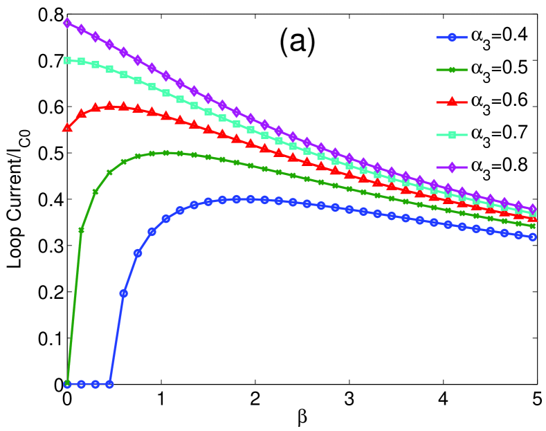
Figure 5(a) shows the magnitude of the loop current $I_{q}$ in the potential minima as a function of $\beta$, where different curves correspond to different $\alpha_{3}$. When $\alpha_{3}<0.5$ and $\beta$ is small enough, the bias flux cannot drive a persistent current in the loop, and a zero-current point ${{\mathbb{P}}}_{0}=(0,0,\pi)\mod 2\pi$ achieves the potential minimum $-\alpha_{1}-\alpha_{2}+\alpha_{3}$. As $\beta$ increases, the loop begins to support a non-zero current. If $\alpha_{3}$ is smaller than a critical value $\bar{\alpha}_{3}=\sqrt{2}/2$, which is obtained by $I_{q}|_{\beta=0}=\alpha_{3}I_{C0}$, the increase of $\beta$ enlarges the loop current to achieve the value $I_{C3}=\alpha_{3}I_{C0}$, the maximum current the loop can afford. In other conditions, a larger inductance always suppresses the loop current. As $\beta$ is large enough, e.g. $\beta=5$, the inductance aggressively erases the differences caused by $\alpha_{3}$ and damps $I_{q}$ into zero quickly, indicating the domination of the inductance $\beta$ in this regime. A simple calculation shows that the phase of every junction tends to be $0$ mod $2\pi$ and, therefore, the $\pi$-phase with which we bias the circuit comes to drop on the loop inductance itself; for example, when $\beta=5$ and $\alpha_{3}=0.8$, the inductance phase $\bar{\phi}$ reaches $0.60\pi$. Actually, when $\beta$ is large enough, a tiny but non-zero current approximately on $O(\Phi_{0}/2L)$ can make the inductance possess almost the external $\pi$-phase bias and force the circuit to approach a possible global potential minimum $-\sum_{k=1}^{3}\alpha_{k}$.

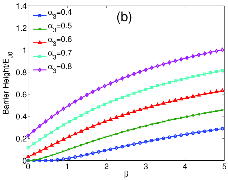
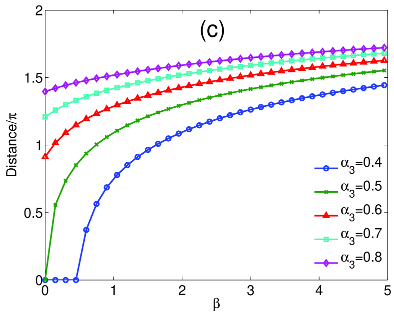
When the circuit begins to support a finite non-zero current in the potential minima, its direction degeneracy yields that the potential minima such as ${{\mathbb{P}}}_{+}=(\bar{\phi}^{+}_{1},\bar{\phi}^{+}_{2},\bar{\phi}^{+}_{3})$, and ${{\mathbb{P}}}_{-}=(-\bar{\phi}^{+}_{1},-\bar{\phi}^{+}_{2},2\pi-\bar{\phi}^{+}_{3})$, where $\bar{\phi}^{+}_{1,2,3}$ belong to the interval of $(0,\pi)$, depart from each other in pair while the zero-current point ${{\mathbb{P}}}_{0}$ pins in the phase space as a saddle point of the barrier, thus forming a double-well potential structure. In this condition, Fig. 5(b) and (c) demonstrate the barrier height defined by the potential difference between ${{\mathbb{P}}}_{+}$ and ${{\mathbb{P}}}_{0}$ and the distance between ${{\mathbb{P}}}_{+}$ and ${{\mathbb{P}}}_{-}$, respectively. It is found that a larger $\beta$ enhances the potential barrier and separates further the well bottoms. Those numerical data verify an intuition that such a non-negligible inductance suppresses the speed of switching the directions of the loop current. Consequently, in the quantum regime, these properties also correspondingly weaken the interactions between the two persistent-current states. See Ref. Robertson2006, for a detailed discussion on the three-phase system as well as its numerical method we utilized.

To study the quantum behaviors of the flux qubit system, the tight-binding model can be utilized in the first step,TJL1999 ; YAM2002 ; Ya2006 and the Hamiltonian of the three-phase flux qubit with proper parameters can be expanded approximately in its two flux states locating in two neighboring potential minima respectively as

$$\hat{H} = {\delta\Phi_{X}{I}_{p}}\sigma_{z}-\Delta\sigma_{x},$$ (146)

where $\sigma_{x}$ and $\sigma_{z}$ are Pauli matrices, $\delta\Phi_{X}$ is the flux deviation from the degeneracy point $\Phi_{X}=0.5\Phi_{0}$, $\Delta>0$ is the tunneling energy between two flux states and ${I}_{p}$ is the magnitude of the characteristic current possessed by the flux states. Define the matrix element $i_{mn}$ of the current operator $\hat{I}_{\phi}$ as $i_{mn}=\langle{m}|\hat{I}_{\phi}|{n}\rangle$ for the $m$th and $n$th eigenstates $|m\rangle$ and $|n\rangle$ with eigenvalues $\varepsilon_{m}$ and $\varepsilon_{n}$, respectively. At $f=0.5$, it yields $2\Delta=\varepsilon_{1}-\varepsilon_{0}$ and $I_{p}$ can be calculated as the magnitude of $i_{10}$. For comparison, the effective theory also gives the corresponding results such as $2\tilde{\Delta}=\tilde{\varepsilon}_{1}-\tilde{\varepsilon}_{0}$, $\tilde{i}_{mn}^{(2)}$, $\tilde{i}_{mn}^{(4)}$, $\tilde{I}_{p}^{(2)}=|\tilde{i}_{01}^{(2)}|_{f=0.5}$ and $\tilde{I}_{p}^{(4)}=|\tilde{i}_{01}^{(4)}|_{f=0.5}$, which we utilize the tilde sign to symbolize in this section. The symbols $\tilde{i}_{mn}^{(2)}$ represent the matrix elements of the effective but non-optimal current operator $\tilde{I}_{\phi}^{(2)}$ and $\tilde{i}_{mn}^{(4)}$ are achieved by the optimal effective current operator $\tilde{I}_{\phi}^{(4)}$. The numerical comparisons are given as follows.

Figure 6: (Color online) Tunnel splitting of the flux qubit, in units of $E_{J0}$, vs. the reduced inductance $\beta$. Parameter $\alpha_{3}$ is selected to be equal to two typical values $0.6$ and $0.8$ while others are $\alpha_{1}=1$, $\alpha_{2}=1$, $g=80$ and $f=0.5$. The inset with the same symbols re-scales the range of $\beta$ and draws the percent changes of the numerical results to the corresponding values on $\beta=0$.

Figure 7: (Color online) Current factors $I_{p}$, ${\tilde{I}_{p}^{(2)}}$ and $\tilde{I}_{p}^{(4)}$ in units of $I_{C0}$ as functions of the reduced inductance $\beta$. The inset plots the deviations of the currents from the corresponding values $I_{p}|_{\beta=0}$ on different $\alpha_{3}$ in per thousand. The parameter $\alpha_{3}$ is also chosen equal to $0.6$ and $0.8$ while the others are $\alpha_{1}=1$, $\alpha_{2}=1$, $g=80$ and $f=0.5$.

Figure 8: (Color online) Relative Errors $\frac{|\tilde{\Delta}-\Delta|}{|\Delta|_{\beta=0}}$ and $\frac{|\tilde{I}^{(4)}_{p}-{I}_{p}|}{|{I}_{p}|_{\beta=0}}$ as functions of the reduced inductance $\beta$.

Figure 9: (Color online) Magnitudes of the current matrix elements $i_{mn}$ for the three lowest levels, in units of $I_{C0}$, vs. the reduced bias flux $f$. Two cases $\beta$=0 and $\beta$=0.5 are selected, and other parameters are $\alpha_{1,2}=1$,$\alpha_{3}=0.8$ and $g=80$.

Figure 10: (Color online) Normalized $|i_{mn}|$, $|\tilde{i}_{mn}^{(2)}|$ and $|\tilde{i}_{mn}^{(4)}|$ as functions of the reduced inductance $\beta$ when $f=0.499$. The data $|{i}_{mn}|$, $|\tilde{i}_{mn}^{(2)}|$ and $|\tilde{i}_{mn}^{(4)}|$ have been divided by the corresponding values $|{i}_{mn}|_{\beta=0}$, and other parameters are $\alpha_{1,2}=1$,$\alpha_{3}=0.8$ and $g=80$. The inset demonstrates a typical error analysis.

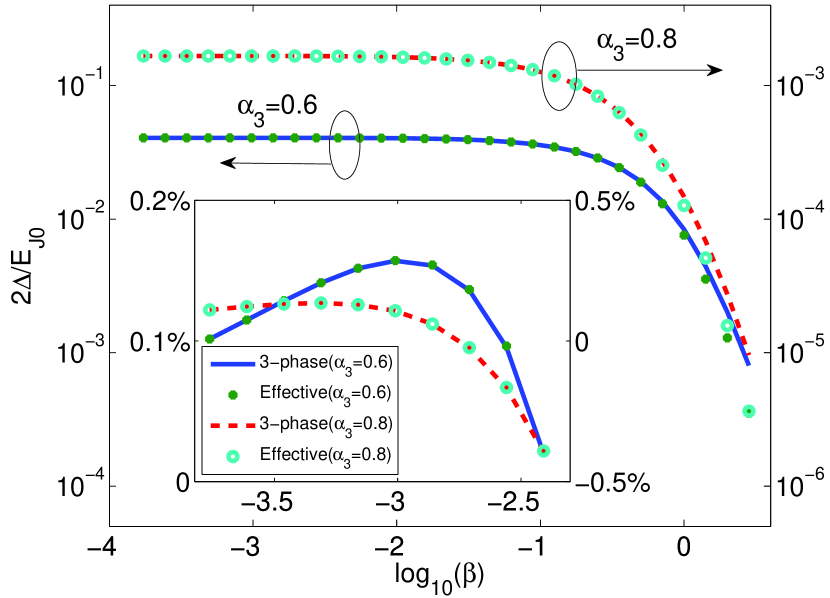
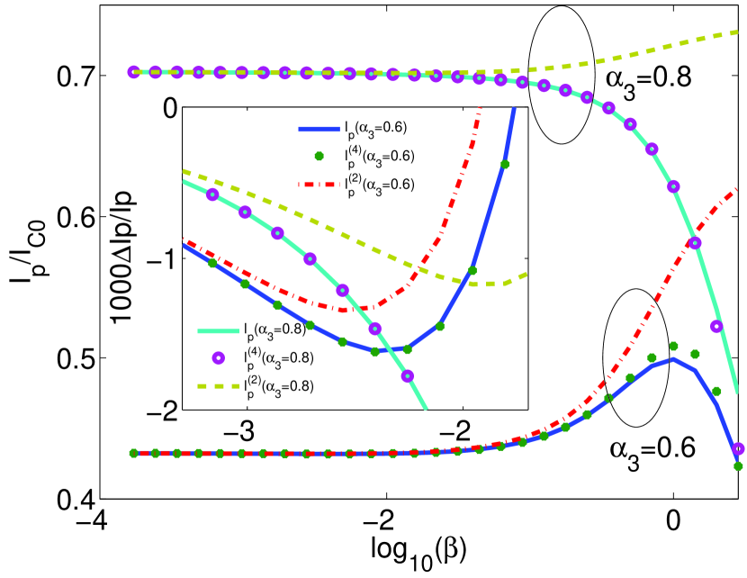
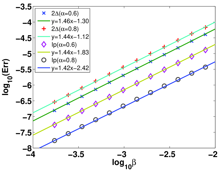
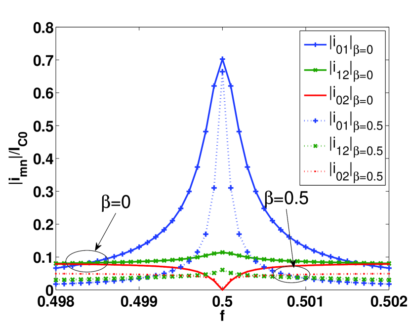
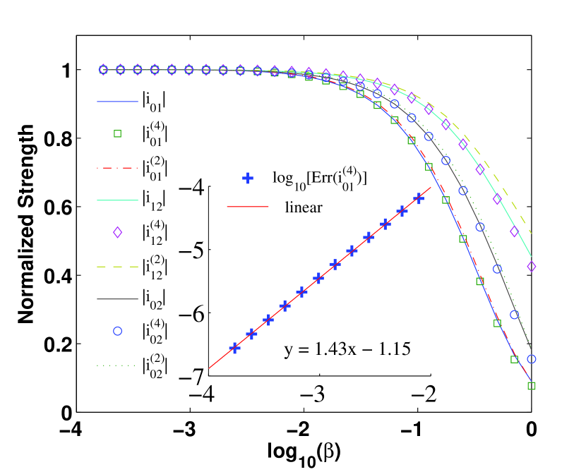
Figure 6 plots $2\Delta$ and $2\tilde{\Delta}$ as functions of $\beta$ based on $\alpha_{3}=0.6$ and $0.8$. When $\beta$ is small enough, e.g., $\beta<0.1$, $2\Delta$ only deviates slightly from its inductance-free value. Furthermore, when $\beta$ is re-scaled (see the inset), it is found that $\Delta$ does not decrease monotonically but reaches its maximum value at $\beta\simeq 10^{-3}$. As mentioned above in the effective theory, the vacuum fluctuations on $O(\beta^{1/2})$ brought by the LC-oscillator actually reduce the effective sizes of the Josephson junctions, thus suppressing the barriers and enhancing the interactions between these two flux states. On the other hand, the self-biased inductive effects like $-LI^{2}/2$ on $O(\beta)$ increase the barriers and slow down the current direction switching speed. As a numerical $order$ prediction, we have those two characteristic factors equal as $\gamma_{1}^{2}\simeq\beta$ and get a critical value $\beta\sim 10^{-3}$ agreeing with the data of the inset. As $\beta$ becomes larger, a clear tunnel rate damping means that the self-biased effects grow up to a non-negligible level. When $\beta>1$, $2\Delta$ is more than one order of magnitude smaller than its inductance-free value, and the effective result $2\tilde{\Delta}$ decays more excessively than $2\Delta$ does; in this situation, a small $\Delta$ means that two flux states of the flux qubit interact with each other weakly and slowly, rendering that the whole system fails to act as a useful qubit in a larger $\alpha_{3}$ such as $\alpha_{3}=0.8$, but $\alpha_{3}=0.6$ only makes the flux qubit slow down which may benefit the design on it with a large loop inductance. It is a pleasure that when the effective Hamiltonian on $O(\beta)$ fails to calculate the inductive effects that involve higher excited levels of the oscillator, the three-phase system with a set of traditional design parameters may no longer perform as a good qubit.

To show the performances of the optimal effective current operator $\tilde{I}_{\phi}^{(4)}$, Fig. 7 depicts the numerical data of ${\tilde{I}_{p}^{(2)}}$, ${\tilde{I}_{p}^{(4)}}$ and $I_{p}$ vs. $\beta$ on the cases of $\alpha_{3}=0.6$ and $\alpha_{3}=0.8$. There is no doubt that $\tilde{I}_{\phi}^{(4)}$ perfectly achieves the results in a high precision regardless of $\alpha_{3}$; even when the inductance has a non-negligible size ($\beta\simeq 1$), it can also correctly predict the profiles of the $I_{p}-\beta$ curves. These curves resemble their classical counterparts $I_{q}$ in Fig. 5(a), which infers us that the shifts of the classical potential minima introduced by a large inductance also take significant roles in the quantum regime. Compared to $I_{p}$ and ${\tilde{I}_{p}^{(4)}}$, $\tilde{I}_{p}^{(2)}$ without full $O(\beta)$ corrections fails to describe $I_{p}$ when the influences imposed by the inductance become notable, e.g. $\beta>0.01$, which also emphasizes that the $O(\beta)$ effects dominate in this region. In fact, the inductive energy term on $O(\beta)$ in $\tilde{H}^{(1)}_{eff}$ tends to make itself minimized averagely in a relatively large $\beta$ region which forces ${\tilde{I}_{p}^{(2)}}$ to rise too pronouncedly to approximate the real value $I_{p}$. As mentioned above, the vacuum fluctuations of the LC oscillator bring in the $O(\beta^{1/2})$ effects and, thus, reduce the effective sizes of the junctions. Therefore, the currents are expected to decline when $\beta$ is small enough to make the $O(\beta)$ effects negligible, which is also confirmed by the inset of Fig. 7. When $\alpha_{3}=0.8$, since the net $O(\beta)$ effects also depress the currents ( see $I_{p}$ when $\beta>0.01$ ), $I_{p}$ and ${\tilde{I}_{p}^{(4)}}$ both monotonously decrease in the whole region. On the other hand, lacking full $O(\beta)$ effects, ${\tilde{I}_{p}^{(2)}}|_{\alpha_{3}=0.8}$ increases in the large $\beta$ region, so there exists a minimum at $\beta\simeq 0.01$ in the corresponding curve when the $O(\beta^{1/2})$ and $O(\beta)$ effects strike a balance. For $\alpha_{3}=0.6$, minima are also found to show the balances between the opposite $O(\beta^{1/2})$ and $O(\beta)$ effects. Both of those two types of minima support our previous conclusion that $\beta\simeq 10^{-3}\sim 10^{-2}$ is the watershed to distinguish the region dominated by the vacuum fluctuations. Figure 8 demonstrates the $\beta$-dependence of the errors which $\tilde{\Delta}$ and $\tilde{I}_{p}^{(4)}$ bear. The linear fitting indicating that these errors are approximately on $O(\beta^{1.5})$ sufficiently verifies our analytic conclusions.

When a small magnitude of time-dependent flux is applied to drive the circuit, the matrix elements $i_{mn}$ contribute to the strengths of the photon-assisted transition rates, significant for the control of the circuit.YJL2005 We consider its three lowest levels and plot the magnitudes of the matrix elements $i_{01,02,12}$ vs. the reduced flux bias $f$ in Fig. 9. When $\beta$ increases to $\beta=0.5$, the $|i_{mn}|$-$f$ curves keep the same shapes approximately except for that their line-widths are much narrower, meaning that it is more difficult to control the circuit. The magnitudes shown in Fig. 10, as $f$ deviates slightly from $f=0.5$, are consistent with our previous conclusion on the weakened interactions, and also indicate that the effective current operator can accurately predict the results even when $\beta$ reaches one. The inset of Fig. 10 also supports our order analysis.

To sum up, the optimal effective current operator describes the loop inductive effects in good agreement with the three-phase full quantum predictions even when the size of the inductance $L$ is comparable with the effective ones’ of the junctions ($\beta\sim 1$) and, consequently, the circuit may perform as a less useful qubit.

VII conclusion

In summary, an optimal effective two-phase current operator for 3jj flux qubit has been obtained if considering the inductance of the circuit loop. In our classical analysis, we have utilized a source transformation to achieve the current form for the inductance-free two-phase system. Then after constructing the Hamiltonian for the three-phase system in the original phase space $(\phi_{1},\phi_{2},\phi_{3})$, we choose a reasonable linear transformation to reformat the Hamiltonian in new variables, where the small inductance phase $\phi$ is separated as a single coordinate, and find that the system can be treated as the inductance-free flux qubit interacting with a high frequency LC-oscillator. Under the condition that the energy of the slow two-phase flux qubit system is small enough comparing to the LC-oscillator’s, an effective theory has been developed for physical variable operators from the photon transition path method based on the BW expansion, which is also suitable for other superconducting circuit types. As an application for the relatively simple results which are still of high accuracy, the effective Hamiltonian is expanded to order $\beta$ and only give an error on $O(\beta^{3/2})$. Besides the direct expansion, enlightened by the classical view on the circuit, we have also presented another simpler method in the effective theory to achieve the explicit form of the optimal current operator $\tilde{I}_{\phi}^{(4)}$ whose corresponding error is merely on the order of $\beta^{3/2}$. Finally, we have verified that the optimal effective operators perfectly describe the numerical properties of the three-phase system.

Appendix A order analysis

For $\hat{H}_{int}$ in Eq. (51), we define its expansion as

$$\langle\Omega_{m}|\hat{H}_{int}|\Omega_{n}\rangle = \sum_{k\geq 1}\hat{\mathcal{V}}_{m,n}^{(k)}\beta^{k/4},$$ (147)

where $\hat{\mathcal{V}}_{m,n}^{(k)}$ are independent of $\beta$. According to the optical selection rules, we have a $\beta^{1/2}$ (instead of $\beta^{1/4}$) series expansion on $\hat{H}_{s,s_{1}}$ as

$$\hat{H}_{s,s_{1}} = \beta^{|s-s_{1}|/4}\sum_{k\geq 0}\hat{\mathcal{V}}_{s,s_{1}}^{(|s-s_{1}|+2k)}\beta^{k/2}\sim{O}(\beta^{|s-s_{1}|/4}),$$ (148)

where the operator $\hat{\mathcal{V}}_{s,s}^{(0)}$ is an alias for the Hamiltonian $\hat{H}_{0}$, and “$\sim{O}(\beta^{|s-s_{1}|/4})$” denotes that the dominant terms in the corresponding operator $\hat{H}_{s,s_{1}}$ are on ${O}(\beta^{|s-s_{1}|/4})$. The operator $\hat{H}_{s,s_{1}}$ combines the effects in proportion to $\beta^{|s-s_{1}|/4}$, $\beta^{|s-s_{1}|/4+1/2}$, $\beta^{|s-s_{1}|/4+1}$ and etc. Generally, the product $\prod_{k=1}^{n}\hat{H}_{s_{k},s_{k-1}}$ $\sim$ $O(\beta^{(\sum_{k=1}^{n}|s_{k}-s_{k-1}|)/4})$ can also be expanded in a $\beta^{1/2}$-series, where $n$ and $s_{k}$ are integers.

Operators $\hat{\mathcal{H}}_{s,s_{1}}$ introduced do not complicate the order analysis on both $\tilde{H}(\varepsilon)$ and $\hat{\mathcal{G}}_{s}(\varepsilon)$. The denominator $s\hbar\omega_{LC}$ is a scale factor in proportion to $\beta^{-1/2}$, and $\varepsilon$ in $\hat{\mathcal{H}}_{s,s}(\varepsilon)$ is dominated by $\varepsilon^{(0)}$ independent of $\beta$. Therefore, one can obtain a typical term $\tilde{H}_{typ}(\varepsilon)$ in $\tilde{H}(\varepsilon)$ as

$$\tilde{H}_{typ}(\varepsilon) = \hat{H}_{0,s_{0}}\hat{\mathcal{H}}_{s_{0},s_{0}}^{i_{0}}(\varepsilon)\hat{\mathcal{H}}_{s_{0},s_{1}}\hat{\mathcal{H}}_{s_{1},s_{1}}^{i_{1}}(\varepsilon)\hat{\mathcal{H}}_{s_{1},s_{2}}...\hat{\mathcal{H}}_{s_{n},s_{n}}^{i_{n}}(\varepsilon)\hat{\mathcal{H}}_{s_{n},0}$$

$$\sim O(\beta^{\frac{n+1}{2}+\frac{1}{2}\Sigma_{k=0}^{n}i_{k}+\frac{1}{4}\Sigma_{k=1}^{n}|s_{k}-s_{k-1}|+\frac{s_{0}}{4}+\frac{s_{n}}{4}}),$$

where $n$, $s_{0}$, $\dots$, $s_{n}$, $i_{0}$, $\dots$ and $i_{n}$ are integers, and $s_{k}\neq s_{k+1}$ for $k$ as an integer. The $\varepsilon$-$\tilde{H}(\varepsilon)$ substitution can change $\tilde{H}(\varepsilon)$ into a $\varepsilon$-independent one on a specific order via using the first few largest $\varepsilon$-less terms like $\hat{H}_{0}$ to replace $\varepsilon$. Mathematically, with $n$ being an integer and $r=n/2$, we can respectively expand the non-Hermitian Hamiltonian $\tilde{H}^{(r)}_{nh}$ to order $\beta^{r}$ and the operator $\hat{\mathcal{G}}_{s}^{(r)}$ to order $\beta^{s/4+r}$ as

$$\tilde{H}^{(r)}_{nh} = \tilde{H}^{(r)}_{nh}|_{\beta^{0}}+\tilde{H}^{(r)}_{nh}|_{\beta^{1/2}}+\tilde{H}^{(r)}_{nh}|_{\beta}+\dots+\tilde{H}^{(r)}_{nh}|_{\beta^{r}}+{\mathit{O}}(\beta^{r+\frac{1}{2}}),$$ (150)

$$\hat{\mathcal{G}}_{s}^{(r)} = \hat{\mathcal{G}}_{s}^{(r)}|_{\beta^{\frac{s}{4}+\frac{1}{2}}}+\hat{\mathcal{G}}_{s}^{(r)}|_{\beta^{\frac{s}{4}+\frac{2}{2}}}+\hat{\mathcal{G}}_{s}^{(r)}|_{\beta^{\frac{s}{4}+\frac{3}{2}}}+\dots$$

$$+\hat{\mathcal{G}}_{s}^{(r)}|_{\beta^{\frac{s}{4}+r}}+O(\beta^{\frac{s}{4}+\frac{1}{2}+r}),$$

where $\tilde{H}^{(r)}_{nh}|_{\beta^{k/2}}\propto\beta^{k/2}$ and $\hat{\mathcal{G}}_{s}^{(r)}|_{\beta^{s/4+k/2}}\propto\beta^{s/4+k/2}$ for the integer $k$. With Eqs. (150) and (A), it can be verified correct that the operator $\hat{\mathcal{G}}_{||}$ in Eq. (84) does not hold any term in proportion to $\beta^{\frac{2k+1}{4}}$ for $k$ as an integer. Therefore, the statement on $\tilde{H}_{eff}$ in Eq. (90) can be justified without any doubt. Since the effective states and their eigenenergy are determined by the effective Hamiltonian $\tilde{H}_{eff}$, we also have $\varepsilon^{(2k+1)}\equiv 0$ and $|\varphi_{0}^{(2k+1)}\rangle\equiv 0$ for $k$ as an integer in Eqs. (53) and (54), respectively.

Appendix B details of operator expansions

In the following sections, $I_{C0}$ is utilized as the current unit, $\hbar=1$ and $e=1/2$. First of all, the operator $\hat{H}_{s,s_{1}}$ ( here $s$ may equate to $s_{1}$ ) in Eq. (61) is

$$\hat{H}_{s,s_{1}} = \hat{H}_{0}\delta_{s,s_{1}}+\langle\Omega_{s}|\left[\sum_{k=1}^{3}\alpha_{k}\cos\theta_{k}-\alpha_{k}\cos\left(\theta_{k}+\frac{\alpha_{ser}}{\alpha_{k}}\phi\right)\right]|\Omega_{s_{1}}\rangle$$

$$= \hat{H}_{0}\delta_{s,s_{1}}+\sum_{k=1}^{3}\alpha_{k}\cos\theta_{k}\delta_{s,s_{1}}-\frac{1}{2}\sum_{k=1}^{3}\left(\alpha_{k}e^{-\frac{\gamma_{k}^{2}}{2}+i\theta_{k}}\sum_{t=0}^{\min(s,s_{1})}\frac{\sqrt{s!s_{1}!}(i\gamma_{k})^{s+s_{1}-2t}}{t!(s-t)!(s_{1}-t)!}+c.c.\right),$$

where $\gamma_{k}=\frac{\alpha_{ser}}{\alpha_{k}}\sqrt[4]{\frac{2\beta}{g\alpha_{ser}}},k=1,2,3$, have been defined in Eq. (99); especially, we have

$$\hat{H}_{0,1} = \sum_{k=1}^{3}\alpha_{k}\gamma_{k}e^{-\frac{\gamma_{k}^{2}}{2}}\sin\theta_{k},$$ (153)

$$\hat{H}_{0,2} = \frac{\sqrt{2}}{2}\sum_{k=1}^{3}\alpha_{k}\gamma_{k}^{2}e^{-\frac{\gamma_{k}^{2}}{2}}\cos\theta_{k}.$$ (154)

Equation (B) as an explicit expression is consistent with the ones in our former order analysis such as Eq. (148). For $s=s_{1}$, the operator $\hat{H}_{s,s}$ holds its dominant term $\hat{H}_{0}$ independent of $\beta$. Since $e^{-\frac{\gamma_{k}^{2}}{2}}=1+O(\beta^{1/2})$ and the largest term among $(i\gamma_{k})^{s+s_{1}-2t}$ in the sum is on $O(\beta^{|s-s_{1}|/4})$ when $t$ equates to $\min(s,s_{1})$, we have the dominant term of $\hat{H}_{s,s_{1}}$ on $O(\beta^{|s-s_{1}|/4})$ for $s\neq s_{1}$. It is due to the optical selection rules that the fluctuation factors $e^{-\frac{\gamma_{k}^{2}}{2}}$ as well as the sums about $(i\gamma_{k})^{s+s_{1}-2t}$ can be expanded in a $\beta^{1/2}$-series. Thus, the operator $\hat{H}_{s,s_{1}}$ is capable to be expanded in the same way. Equation (B) also yields

$$\hat{H}_{0,0}=\hat{H}_{s,s}+O(\beta^{1/2}),$$ (155)

where $s\neq 0$, and the terms in proportion to $\beta^{1/4}$ miss due to the optical selection rules.

We expand $\hat{\mathcal{G}}_{1,2,3}(\varepsilon)$ as follows,

$$\hat{\mathcal{G}}_{1}(\varepsilon) = \hat{\mathcal{H}}_{1,0}+\hat{\mathcal{H}}_{1,1}(\varepsilon)\hat{\mathcal{H}}_{1,0}+\hat{\mathcal{H}}_{1,1}^{2}(\varepsilon)\hat{\mathcal{H}}_{1,0}+\hat{\mathcal{H}}_{1,2}\hat{\mathcal{H}}_{2,0}+O(\beta^{9/4})$$

$$= -\frac{\hat{H}_{1,0}}{\hbar\omega_{LC}}+\frac{(\hat{H}_{1,1}-\varepsilon)\hat{H}_{1,0}}{(\hbar\omega_{LC})^{2}}-\frac{(\hat{H}_{1,1}-\varepsilon)^{2}\hat{H}_{1,0}}{(\hbar\omega_{LC})^{3}}+\frac{\hat{H}_{1,2}\hat{H}_{2,0}}{2(\hbar\omega_{LC})^{2}}+O(\beta^{9/4})$$

$$= -\frac{\hat{H}_{1,0}}{\hbar\omega_{LC}}+\frac{\hat{H}_{1,1}\hat{H}_{1,0}-\hat{H}_{1,0}\hat{H}_{0,0}}{(\hbar\omega_{LC})^{2}}-\frac{\left[\hat{H}_{0},\left[\hat{H}_{0},\hat{H}_{1,0}\right]\right]}{(\hbar\omega_{LC})^{3}}$$

$$+\frac{\hat{H}_{1,2}\hat{H}_{2,0}}{2(\hbar\omega_{LC})^{2}}+O(\beta^{9/4}),$$

$$\hat{\mathcal{G}}_{2}(\varepsilon) = \hat{\mathcal{H}}_{2,0}+\hat{\mathcal{H}}_{2,2}(\varepsilon)\hat{\mathcal{H}}_{2,0}+\hat{\mathcal{H}}_{2,1}\hat{\mathcal{H}}_{1,0}+O(\beta^{8/4})$$

$$= -\frac{\hat{H}_{2,0}}{2\hbar\omega_{LC}}+\frac{(\hat{H}_{2,2}-\varepsilon)\hat{H}_{2,0}}{4(\hbar\omega_{LC})^{2}}+\frac{\hat{H}_{2,1}\hat{H}_{1,0}}{2(\hbar\omega_{LC})^{2}}+O(\beta^{8/4})$$

$$= -\frac{\hat{H}_{2,0}}{2\hbar\omega_{LC}}+\frac{\left[\hat{H}_{0},\hat{H}_{2,0}\right]}{4(\hbar\omega_{LC})^{2}}+\frac{\hat{H}_{2,1}\hat{H}_{1,0}}{2(\hbar\omega_{LC})^{2}}+O(\beta^{8/4}),$$

$$\hat{\mathcal{G}}_{3}(\varepsilon) = \hat{\mathcal{H}}_{3,0}+O(\beta^{7/4})=-\frac{\hat{H}_{3,0}}{3\hbar\omega_{LC}}+O(\beta^{7/4}),$$ (158)

where since from the effective Hamiltonian we know that

$$\tilde{H}(\varepsilon)=\hat{H}_{0}+O(\beta^{1/2})=\hat{H}_{0,0}+O(\beta),$$ (159)

we utilize the $\varepsilon$-$\tilde{H}(\varepsilon)$ substitutions on specific orders of $\beta$ as follows:

$$\frac{\varepsilon\hat{H}_{1,0}}{(\hbar\omega_{LC})^{2}}|\varphi_{0}\rangle = \frac{\hat{H}_{1,0}\tilde{H}(\varepsilon)}{(\hbar\omega_{LC})^{2}}|\varphi_{0}\rangle=\frac{\hat{H}_{1,0}\hat{H}_{0,0}}{(\hbar\omega_{LC})^{2}}|\varphi_{0}\rangle+O(\beta^{9/4}),$$ (160)

$$\frac{(\hat{H}_{1,1}-\varepsilon)^{2}\hat{H}_{1,0}}{(\hbar\omega_{LC})^{3}}|\varphi_{0}\rangle = \frac{(\hat{H}_{1,1}^{2}+\varepsilon^{2}-2\hat{H}_{1,1}\varepsilon)\hat{H}_{1,0}}{(\hbar\omega_{LC})^{3}}|\varphi_{0}\rangle$$

$$= \frac{\hat{H}_{1,1}^{2}\hat{H}_{1,0}+\hat{H}_{1,0}\tilde{H}(\varepsilon)^{2}-2\hat{H}_{1,1}\hat{H}_{1,0}\tilde{H}(\varepsilon)}{(\hbar\omega_{LC})^{3}}|\varphi_{0}\rangle$$

$$= \frac{\left[\hat{H}_{0},\left[\hat{H}_{0},\hat{H}_{1,0}\right]\right]}{(\hbar\omega_{LC})^{3}}|\varphi_{0}\rangle+O(\beta^{9/4}),$$

$$\frac{\varepsilon\hat{H}_{2,0}}{4(\hbar\omega_{LC})^{2}}|\varphi_{0}\rangle = \frac{\hat{H}_{2,0}\tilde{H}(\varepsilon)}{4(\hbar\omega_{LC})^{2}}|\varphi_{0}\rangle=\frac{\hat{H}_{2,0}\hat{H}_{0}}{4(\hbar\omega_{LC})^{2}}|\varphi_{0}\rangle+O(\beta^{8/4}).$$ (162)

Appendix C solution of generalized eigen-problem

For the generalized eigen-problem, due to the perturbations, the positive and Hermitian operator $\hat{R}$ suggests that Eq. (77) can be converted to an eigen-problem as

$$\hat{R}^{-\frac{1}{2}}\tilde{H}^{(3/2)}_{L}\hat{R}^{-\frac{1}{2}}\left(\hat{R}^{\frac{1}{2}}|\varphi_{0}\rangle\right) = \varepsilon\left(\hat{R}^{\frac{1}{2}}|\varphi_{0}\rangle\right)+O(\beta^{2}),$$ (163)

where the initial “$+O(\beta^{7/4})$” has been improved to “$+O(\beta^{2})$” due to the previous discussions on the optical selection rules. Expanding $\hat{R}$ to order $\beta^{3/2}$ in Eq. (163) yields

$$\tilde{H}^{(3/2)}_{eff}|\varphi_{eff}^{(3/2)}\rangle = \varepsilon|\varphi_{eff}^{(3/2)}\rangle+O(\beta^{2}),$$ (164)

where an effective Hamiltonian $\tilde{H}^{(3/2)}_{eff}$ independent of $\varepsilon$ reads

$$\tilde{H}^{(3/2)}_{eff} = \hat{H}_{0,0}-\frac{\hat{H}_{0,1}\hat{H}_{1,0}}{\hbar\omega_{LC}}-\frac{\hat{H}_{0,2}\hat{H}_{2,0}}{2\hbar\omega_{LC}}+\frac{\hat{H}_{0,1}\hat{H}_{1,1}\hat{H}_{1,0}}{(\hbar\omega_{LC})^{2}}$$

$$-\frac{1}{2}\frac{\hat{H}_{0,1}\hat{H}_{1,0}\hat{H}_{0,0}+\hat{H}_{0,0}\hat{H}_{0,1}\hat{H}_{1,0}}{(\hbar\omega_{LC})^{2}},$$

and the effective eigenstate $|\varphi_{eff}^{(3/2)}\rangle$ is

$$|\varphi_{eff}^{(3/2)}\rangle = \left(1+\frac{1}{2}\frac{\hat{H}_{0,1}\hat{H}_{1,0}}{(\hbar\omega_{LC})^{2}}\right)|\varphi_{0}\rangle.$$ (166)

The effective Hamiltonian $\tilde{H}^{(3/2)}_{eff}$ is Hermitian since the transformation $\left(\hat{R}^{-\frac{1}{2}}\cdot\hat{R}^{-\frac{1}{2}}\right)$ does not alter the Hermiticity of $\tilde{H}^{(3/2)}_{L}$. One remarkable thing is that $|\varphi_{eff}^{(3/2)}\rangle$ is naturally normalized on $O(\beta^{3/2})$. Since the eigenstate $|\varphi\rangle$ is normalized as $\langle\varphi|\varphi\rangle=1$, we expand it to order $\beta^{3/2}$ and have

$$1=\langle\varphi|\varphi\rangle=\langle\varphi_{eff}^{(3/2)}|\varphi_{eff}^{(3/2)}\rangle+O(\beta^{2}).$$ (167)

In sum, Eq. (164) is consistent with Eq. (94) as an eigen-problem which covers the eigenstates in the manifold $\mathcal{M}_{0}$ for the whole three-phase system on $O(\beta^{3/2})$.

Appendix D proofs of Hermiticity of $\tilde{H}_{eff}$

First, let us calculate the value of the operator $\hat{D}$

$$\hat{D}=\hat{\mathcal{G}}_{||}^{2}\tilde{H}_{nh}-\tilde{H}_{nh}^{{\dagger}}\hat{\mathcal{G}}_{||}^{2},$$ (168)

According to Eqs. (82) and (85), applying $\langle\psi_{0}|\cdot|\varphi_{0}\rangle$ to Eq. (168) yields

$$\langle\psi_{0}|\hat{D}|\varphi_{0}\rangle = \langle\psi_{0}|\hat{\mathcal{G}}_{||}^{2}\tilde{H}_{nh}|\varphi_{0}\rangle-\langle\psi_{0}|\tilde{H}_{nh}^{{\dagger}}\hat{\mathcal{G}}_{||}^{2}|\varphi_{0}\rangle$$

$$= (\varepsilon_{\varphi}-\varepsilon_{\psi})\delta_{\psi,\varphi}$$

$$\equiv 0.$$

Assuming the dominant term $\hat{D}^{(k)}$ of $\hat{D}$ is proportional to $\beta^{k/4}$ with $k$ being an integer, we can expand Eq. (D) to order $\beta^{k/4}$ as

$$\langle\psi_{0}^{(0)}|\hat{D}^{(k)}|\varphi_{0}^{(0)}\rangle\equiv 0.$$ (170)

As the projected components $|\psi_{0}^{(0)}\rangle$ and $|\varphi_{0}^{(0)}\rangle$ are arbitrary eigenstates of the unperturbed Hamiltonian $\hat{H}_{0}$, it yields

$$\hat{D}^{(k)}\equiv 0,$$ (171)

and, thus,

$$\hat{D}\equiv 0,$$ (172)

for $k$ being arbitrary. It follows that

$$\hat{\mathcal{G}}_{||}^{2}\tilde{H}_{nh}=\tilde{H}_{nh}^{{\dagger}}\hat{\mathcal{G}}_{||}^{2}.$$ (173)

Finally, we achieve that

$$\tilde{H}_{eff} = \hat{\mathcal{G}}_{||}\tilde{H}_{nh}\hat{\mathcal{G}}_{||}^{-1}$$

$$= \hat{\mathcal{G}}_{||}^{-1}\tilde{H}_{nh}^{{\dagger}}\hat{\mathcal{G}}_{||}$$

$$= \tilde{H}_{eff}^{{\dagger}}.$$

Appendix E calculations on effective operators

For the charge operator

$$\hat{Q}_{\phi} = i\sqrt[4]{\frac{\alpha_{ser}g}{2\beta}}\frac{\hat{a}^{{\dagger}}-\hat{a}}{2},$$ (175)

we have its effective operator on $O(\beta)$ as

$$\tilde{Q}_{\phi} = i\sqrt[4]{\frac{\alpha_{ser}g}{2\beta}}\frac{\hat{\mathcal{G}}_{1}^{{\dagger}}-\hat{\mathcal{G}}_{1}}{2}+O(\beta^{3/2})$$

$$= \frac{i\beta\alpha_{ser}g}{8}{\left[\tilde{I}_{\phi}^{(2)},\hat{H}_{0}\right]}+O(\beta^{3/2}).$$

With $|\varphi\rangle$, $|\psi\rangle$, $\varepsilon_{\varphi}$ and $\varepsilon_{\psi}$ being defined in Sec. IV.4, we apply $\langle\psi|\cdot|\varphi\rangle$ to $\dot{Q}_{\phi}$ and expand it on $O(\beta)$ as

$$\langle\psi|\dot{Q}_{\phi}|\varphi\rangle = \langle\psi|\left[\hat{H}_{tr},i\hat{Q}_{\phi}\right]|\varphi\rangle$$

$$= i(\varepsilon_{\psi}-\varepsilon_{\varphi})\langle\psi|\hat{Q}_{\phi}|\varphi\rangle$$

$$= \frac{-\beta\alpha_{ser}g(\varepsilon_{\psi}-\varepsilon_{\varphi})}{8}\langle\psi_{0}|{\left[\tilde{I}_{\phi}^{(2)},\hat{H}_{0}\right]}|\varphi_{0}\rangle+O(\beta^{3/2})$$

$$= \left(\frac{\varepsilon_{\psi}-\varepsilon_{\varphi}}{\hbar\omega_{LC}}\right)^{2}\langle\psi_{0}|\tilde{I}_{\phi}^{(2)}|\varphi_{0}\rangle+O(\beta^{3/2})$$

$$= \langle\psi_{0}|\left(\frac{\varepsilon_{\psi}^{2}\tilde{I}_{\phi}^{(2)}+\tilde{I}_{\phi}^{(2)}\varepsilon_{\varphi}^{2}-2\varepsilon_{\psi}\tilde{I}_{\phi}^{(2)}\varepsilon_{\varphi}}{\left(\hbar\omega_{LC}\right)^{2}}\right)|\varphi_{0}\rangle+O(\beta^{3/2})$$

$$= \langle\psi_{0}|\left(\frac{\hat{H}_{0}^{2}\tilde{I}_{\phi}^{(2)}+\tilde{I}_{\phi}^{(2)}\hat{H}_{0}^{2}-2\hat{H}_{0}\tilde{I}_{\phi}^{(2)}\hat{H}_{0}}{\left(\hbar\omega_{LC}\right)^{2}}\right)|\varphi_{0}\rangle+O(\beta^{3/2}),$$

where we utilize

$$\hat{H}_{0}|\varphi_{0}\rangle=\varepsilon_{\varphi}|\varphi_{0}\rangle+O(\beta^{1/2}),$$ (178)

$$\hat{H}_{0}|\psi_{0}\rangle=\varepsilon_{\psi}|\psi_{0}\rangle+O(\beta^{1/2}).$$ (179)

Therefore, we have

$$\dot{Q}_{\phi}^{eff} = \frac{\hat{H}_{0}^{2}\tilde{I}_{\phi}^{(2)}+\tilde{I}_{\phi}^{(2)}\hat{H}_{0}^{2}-2\hat{H}_{0}\tilde{I}_{\phi}^{(2)}\hat{H}_{0}}{\left(\hbar\omega_{LC}\right)^{2}}+O(\beta^{3/2}),$$ (180)

which is the same as Eq. (144).

References

- (1) Y. Makhlin, G. Schön, and A. Shnirman, Rev. Mod. Phys. 73, 357 (2001).
- (2) M. H. Devoret, A. Wallraff, and J. M. Martinis, cond-mat/0411174.
- (3) G. Wendin and V. Shumeiko, cond-mat/0508729.
- (4) T. P. Orlando, J. E. Mooij, L. Tian, C. H. van der Wal, L. Levitov, S. Lloyd, and J. J. Mazo, Phys. Rev. B 60, 15398 (1999).
- (5) J. E. Mooij, T. P. Orlando, L. Levitov, Lin Tian, Caspar H. van der Wal, and S. Lloyd, Science 285, 1036 (1999).
- (6) C. H. van der Wal, A. C. J. ter Haar, F. K. Wilhelm, R. N. Schouten, C. J. P. M. Harmans, T. P. Orlando, S. Lloyd, and J. E. Mooij, Science 290, 773 (2000).
- (7) I. Chiorescu, Y. Nakamura, C. J. P. M. Harmans, and J. E. Mooij, Science 299, 1869 (2003).
- (8) I. Chiorescu, P. Bertet, K. Semba, Y. Nakamura, C. J. P. M. Harmans, and J. E. Mooij, Nature 431, 159 (2004).
- (9) W. D. Oliver, Y. Yu, J. C. Lee, K. K. Berggren, L. S. Levitov, and T. P. Orlando, Science 310, 1653 (2005).
- (10) J. H. Plantenberg, P. C. de Groot, C. J. P. M. Harmans and J. E. Mooij, Nature 447, 836 (2007).
- (11) D. M. Berns, M. S. Rudner, S. O. Valenzuela, K. K. Berggren, W. D. Oliver, L. S. Levitov and T. P. Orlando, Nature 455, 51 (2008).
- (12) J. B. Majer, F. G. Paauw, A.C.J. ter Haar, C. J. P.M. Harmans and J. E. Mooij, Phys. Rev. Lett. 94, 090501 (2005).
- (13) J. Q. You, Y. Nakamura, and F. Nori, Phys. Rev. B 71, 024532 (2005).
- (14) A. Maassen van den Brink, Phys. Rev. B 71, 064503 (2005).
- (15) M. Grajcar, A. Izmalkov, S. H. W. van der Ploeg, S. Linzen, T. Plecenik, T. Wagner, U. Hbner, E. Il’ichev, H. G. Meyer, A.Y. Smirnov,P. J. Love, A. Maassen van den Brink, M. H. S. Amin, S. Uchaikin, and A. M. Zagoskin, Phys. Rev. Lett 96, 047006 (2006).
- (16) Y. X. Liu, C. P. Sun and F. Nori, Phys. Rev. A 74, 052321 (2006).
- (17) Y. X. Liu, L. F. Wei, J. R. Johansson, J. S. Tsai, and F. Nori, Phys. Rev. B 76, 144518 (2007).
- (18) G. Burkard, R. H. Koch, and D. P. DiVincenzo, Phys. Rev. B 69, 064503 (2004).
- (19) G. Burkard, D. P. DiVincenzo, P. Bertet, I. Chiorescu, and J. E. Mooij, Phys. Rev. B 71, 134504 (2005).
- (20) D. S. Crankshaw and T. P. Orlando, IEEE Trans. Appl. Supercond. 11, 1006 (2001).
- (21) Y. S. Greenberg, cond-mat/0601493.
- (22) T. L. Robertson, B. L. T. Plourde, P. A. Reichardt, T. Hime, C.-E. Wu, and John Clarke, Phys. Rev. B 73, 174526 (2006).
- (23) L. Tian, A Superconducting Flux Qubit: Measurement, Noise, and Control, Doctoral Thesis. (Massachusetts Institute of Technology, 2002).
- (24) Y. X. Liu, J. Q. You, L. F. Wei, C. P. Sun, and F. Nori, Phys. Rev. Lett. 95, 087001 (2005).
- (25) Y. Yu, W. D. Oliver, J. C. Lee, K. K. Berggren, L. S. Levitov, and T. P. Orlando, cond-mat/0508587.
- (26) J.J. Boyle, and M.S. Pindzola, Many-body atomic physics : lectures on the application of many-body theory to atomic physics. (Cambridge University Press, New York, 1998).
- (27) Tao Wu, Zheng Li, and Jianshe Liu, Jpn. J. Appl. Phys. 45, L180 (2006).
- (28) C. Cohen-Tannoudji, J. Dupont-Roc, and G. Grynberg, Atom-Photon Interactions. (John Wiley & Sons, New York, 1992).
- (29) D. J. Klein, J. Chem. Phys. 61, 786 (1973).
- (30) C. K. Duan, and M. F. Reid, J. Chem. Phys. 115, 8279 (2001).
- (31) A. L. Chernyshev, D. Galanakis, P. Phillips, A. V. Rozhkov, and A.-M. S. Tremblay, Phys. Rev. B 70, 235111 (2004).
- (32) Y. S. Greenberg, A. Izmalkov, M. Grajcar, E. Il’ichev, W. Krech, H. G. Meyer, M. H. S. Amin, and A. Maassen van den Brink, Phys. Rev. B 66, 214525 (2002).