Chemical reactions in the presence of surface modulation and stirring

Abstract

We study the dynamics of simple reactions where the chemical species are confined on a general, time-modulated surface, and subjected to externally-imposed stirring. The study of these inhomogeneous effects requires a model based on a reaction-advection-diffusion equation, which we derive. We use homogenization methods to show that up to second order in a small scaling parameter, the modulation effects on the concentration field are asymptotically equivalent for systems with or without stirring. This justifies our consideration of the simpler reaction-diffusion model, where we find that by modulating the substrate, we can modify the reaction rate, the total yield from the reaction, and the speed of front propagation. These observations are confirmed in three numerical case studies involving the autocatalytic and bistable reactions on the torus and a sinusoidally-modulated substrate. EES classification: 100.000, 110.000

1 Introduction

We investigate the dynamics of the logistic and bistable reactions on a generalized, time-varying substrate with stirring. Such spatially-inhomogeneous problems call for the solution of a reaction-advection-diffusion equation, and much chemical and biological activity in fluid flow can be modelled by such equations. In particular, problems concerning autocatalytic chemical reactions Strogatz1994 and population dynamics Skellam1951 ; Murray1993 possess a logistic growth function as a reaction term, and thus satisfy a Fisher-KPP type of equation. Other, more complicated growth functions can be used to model a variety of phenomena, including the spread of insect populations, or the propagation of electro-chemical waves in organisms Murray1993 . The original motivation of this study was to understand the effects of wave modulation on the population dynamics of plankton, although the language and techniques we use are quite general.

Before deriving and analyzing our model, we place our work in context by examining several streams of work that are relevant. It is known that a growing domain can modify biological pattern formation, as evidenced by the work of Newman and Frisch Newman1979 . This has given impetus to the study of reaction-diffusion equations on growing domains Kondo1995 ; Crampin1999 in one dimension. Logically, this has led to the study of such problems on manifolds embedded in three dimensions. In multiple dimensions, one considers either the effect of curvature Gomatam1997 ; Varea1999 ; Chaplain2001 , or the twin effects of domain growth and curvature Plaza2004 ; Gjorgjieva2007 . The paper of Plaza et al. Plaza2004 is particularly relevant to the present work. In it, the authors derive the reaction-diffusion equation for a class of manifolds, and then study pattern formation on growing domains. We re-work their derivation to include the most general two-dimensional (differentiable) manifold possible, and then shift the focus from pattern formation to reactions in the presence of stirring. The geometric formalism of Aris Aris1962 is central to our derivation. These references Plaza2004 ; Gjorgjieva2007 consider the ‘geometric sink’, that is, the notion that a growing domain can act as a sink for the chemical reaction. We extend this idea to growing and modulating domain sizes and examine the effects of the sink through numerical simulation.

The notion of flow-driven reactions is not new. In Neufeld2001 , the effects of chaotic advection on the Fitz Hugh–Nagumo model are considered. The flow is found to produce a coherent global excitation of the system, for a certain range of stirring rates. The effects of flow can also induce distinctive spatial structure in the chemical concentration; this is studied in Neufeld1999 . The same authors examine the single-component logistic or Fisher-KPP model in Neufeld2001 . There the focus is on regime-change, namely how the rate of chaotic advection affects the spatial structure of the concentration. For slow stirring / fast reactions, a spatially inhomogeneous perturbation decays rapidly, and the equilibrium state is reached rapidly. On the other hand, for fast stirring / slow reactions, the perturbation persists, and a filament structure propagates throughout the domain. Nevertheless, the asymptotic state is still a stable homogeneous one. This system is simplified and the the transition treated as a bifurcation problem in Menon2005 . The focus of these papers is on local temporal and spatial structure. It is therefore salutary to examine the paper of Birch et al. Birch2007 , where the authors examine the averaged effect of a non-constant growth rate on the dynamics of the stirred Fisher-KPP equation. The authors use the theory of estimates to obtain bounds on the reaction yield, as a function of the stirring and the non-constant growth rate. When the mean growth rate is negative, the previously-unstable zero state of the Fisher-KPP equation can become stable; then the catalyst fails to propagate the reaction. In the Birch paper, the inhomogeneous growth rate is the consequence of an inhomogeneous distribution of nutrient in a plankton population. It could, however, be the result of placing the population or chemical species on a modulating surface, which is the subject of our report. Indeed, our results demonstrate the possibility of increasing the reaction yield by surface modulation.

If the flow field or the modulation have small length scales compared to the domain size, then homogenization theory naturally presents itself as a tool for understanding the effects of flow and modulation in an averaged sense Pavliotis2008 . The small scales are bundled up into an effective diffusion constant, and the model reduces to a more manageable equation involving a diffusion operator. Such an approach has been used in the linear advection-diffusion equation McLaughlin1985 ; McCarty1988 ; Rosencrans1997 , for linear reaction-advection-diffusion equations Papanicolaou95 , and for non-linear equations Bensoussan1978 . We propose and justify the application of this theory to a linearized, advective Fisher-KPP equation on a time-varying manifold, and compute the effective diffusivity for the torus. The effective diffusivity for a manifold is, in general, a function of position, although in the fortuitous case we consider, this dependence vanishes. As in Neufeld2002 , the asymptotic state of the system is homogeneous, and the purpose of our homogenization calculation is therefore to study the speed at which this state is reached.

This paper is organized as follows. In Sec. 2 we discuss the autocatalytic reaction in the homogeneous case, and then generalize this formalism to consider reactions on time-dependent, spatially-inhomogeneous surfaces. In Sec. 3 we derive conditions on the metric tensor for homogeneous solutions to exist on a general surface. We then outline a separation-of-scales technique that enables us to compute the spatial distribution of concentration as the solution of a diffusion equation. We discuss the case of shear flow on a modulating torus, where the equation for the effective diffusion is remarkably simple. In Sec. 4 we outline three case studies for unstirred mixtures. We demonstrate that modulating the surface can increase the reaction yield. We verify that this result is independent of the reaction type by obtaining a similar result for the bistable reaction function. Finally, in Sec. 5 we present our conclusions.

2 Theoretical formulation

In this section we describe the mathematical formulation for the autocatalytic reaction. We derive the rate equation for homogeneous concentrations, and then generalize this result to spatially-varying concentrations on generalized two-dimensional surfaces. We pay close attention to understanding the effect on the reaction rate when the surface itself varies with time.

In the homogeneous case, the evolution of $n$ chemical species whose concentrations are given by the vector $\bm{C}=(c_{1}(t),c_{2}(t),...,c_{n}(t))$ can be placed in the following canonical form:

$$\frac{d\bm{C}}{dt}=\bm{F}\left(\bm{C}\right),$$ (2.1)

where the $n$-vector of functions $\bm{F}$ is the reaction term describing the interactions between the different species. We are interested in particular in the autocatalytic reaction $c_{1}+c_{2}\longrightarrow 2c_{2}$; the dynamical system for such a reaction is given by the equation pair

$$\frac{dc_{1}}{dt}=-\beta c_{1}c_{2},\;\frac{dc_{2}}{dt}=\beta c_{1}c_{2},$$ (2.2)

where $\beta>0$ is the reaction rate. The implied equation $d(c_{1}+c_{2})/{dt}=0$ is a statement of molecular conservation. This system is reduced to a single equation by defining a new variable $c=c_{2}/\left(c_{1}+c_{2}\right)$, giving rise to the logistic growth law

$$\frac{dc}{dt}=\sigma c(1-c),$$ (2.3)

where $F(c)=\sigma c(1-c)$ is the reaction function and $\sigma\equiv\beta(c_{1}+c_{2})>0$ is the associated rate. The evolution of this relative concentration is a contest between linear creation and quadratic destruction, which manifests itself through the sigmoid solution $c=c(0)e^{\sigma t}/\left[1+c(0)(e^{\sigma t}-1)\right]$, where $c(0)>0$ is the initial concentration.

The two critical points satisfying ${dc}/{dt}=0$ are the states $c=0$ and $c=1$, respectively indicating when species $c_{2}$ is extinct and when the whole space of concentrations is equal to that of the product $c_{2}$; i.e. $c_{1}$ is extinct. Since ${\partial F}/{\partial c}=\sigma(1-2c)$, $c=0$ is unstable and $c=1$ is stable. The phase portrait of the one-dimensional dynamical system is easily envisioned: there is a quadratically-increasing reaction away from the repeller $c=0$, towards larger values of $c$. When the product is half of the whole concentration mix $c=1/2$; the reaction rate is maximal, and thereafter it decreasess quadratically towards the attractor at $c=1$. Hence, if we start with a soup composed of only $c_{1}$-molecules, the addition of any amount of the second species (no matter how small) leads to the annihilation of the first, while in the reversed scenario it is what is added, in this case the $c_{1}$-molecules, that will be destroyed. Any mixture of the two tends towards a homogeneous soup wholly composed of the species $c_{2}$.

We can generalize the mass-action law to the inhomogeneous case by using the following assumptions:

• There is diffusion of concentration, arising from thermodynamic fluctuations;

• There is a large-scale imposed stirring, modelled as an advecting velocity;

• The substrate $\mathcal{M}$ on which the substance is placed is modulated as a function of time.

We write down a continuity equation that takes account of these features. The approach we take was discussed by Aris Aris1962 , although the application to reaction-diffusion systems is new. We examine the mass balance for the chemical concentration with respect to a control area $S\left(t\right)$. We work with a general two-dimensional manifold $\mathcal{M}$. At time $t=0$ the manifold is endowed with co-ordinates $\bm{a}_{0}$, such that

$$\mathcal{M}\left(0\right)=\{\bm{x}\in\mathbb{R}^{3}|\bm{x}=\bm{x}\left(a_{0}^{1},a_{0}^{2}\right)\},$$

These co-ordinates can be used to label the fluid particles at time $t=0$. As time evolves, the fluid particles are advected by an imposed flow $\bm{U}$, and the particle labels develop time-dependence, $\bm{a}\left(t\right)$. We introduce another set of co-ordinates denoted by $\bm{q}\left(t\right)$. These are fixed in the sense that a point in $\mathbb{R}^{3}$, if located by the co-ordinates $\bm{q}\left(t\right)$, has an instantaneous velocity wholly normal to the surface $\mathcal{M}\left(t\right)$. Since the manifold varies smoothly in time, there is a set of transformations connecting these co-ordinate systems:

$$\bm{q}=\bm{q}\left(\bm{a},t\right),\qquad\bm{a}=\bm{a}\left(\bm{q},t\right),\qquad\bm{a}_{0}=\bm{a}\left(\bm{q}\left(0\right),0\right).$$ (2.4)

A particle that is advected from an initial point $\bm{a}_{0}$ by the imposed stirring $\bm{U}$ therefore has a velocity

$$\bm{U}\left(\bm{q},t\right)=\left(\frac{\partial\bm{q}}{\partial t}\right)_{\bm{a}}\equiv\frac{d\bm{q}}{dt},$$

where, by Eq. (2.4), the time derivative is taken at fixed particle label $\bm{a}$. The last piece of formalism needed is the prescription of a metric tensor:

$$g_{ij}\left(\bm{q},t\right)=\frac{\partial\bm{x}}{\partial q^{i}}\cdot\frac{\partial\bm{x}}{\partial q^{i}}=\bm{g}_{(i)}\cdot\bm{g}_{(j)},\qquad g=\mathrm{det}\left(g_{ij}\right),$$ (2.5)

and the fixedness of the co-ordinate system $\bm{q}$ is thus made manifest:

$$\bm{g}_{(i)}\cdot\left(\frac{\partial\bm{x}}{\partial t}\right)_{\bm{q}}\equiv\,\,\bm{g}_{(i)}\cdot\frac{\partial\bm{x}}{\partial t}=0,\qquad i=1,2.$$

Using the transformations (2.4) and the metric tensor (2.5), we obtain a convenient definition of area, either as an integral over a fixed domain, or a time-varying one:

$$\int_{S\left(t\right)}dS=\int_{S\left(t\right)}\sqrt{|g|}dq^{1}dq^{2}=\int_{S\left(0\right)}\sqrt{|g|}Jda^{1}da^{2},$$

where $S\left(0\right)$ is the pre-advected domain and

$$J=\frac{\partial\left(q^{1},q^{2}\right)}{\partial\left(a^{1},a^{2}\right)}$$

is the Jacobian of the transformation. This formalism facilitates the derivation of an analog of the Reynolds transport theorem for a concentration field $c\left(\bm{q}\left(t\right),t\right)$ Aris1962 ; Bicak1999 ; Hu2007 :

$$\frac{d}{dt}\int_{S\left(t\right)}c\,dS = \int_{S\left(t\right)}\left[\left(\frac{\partial c}{\partial t}\right)_{\bm{a}}+c\left(\frac{\partial}{\partial t}\log\sqrt{|g|}\right)_{\bm{a}}\right]dS,$$ (2.6)

$$= \int_{S\left(t\right)}\left[\left(\frac{\partial c}{\partial t}\right)_{\bm{q}}+\mathrm{div}\left(\bm{U}c\right)+c\left(\frac{\partial}{\partial t}\log\sqrt{|g|}\right)_{\bm{q}}\right]dS.$$

This change in the amount of concentration in the control patch must be matched by the diffusive flux through the boundary of the patch, and by the amount

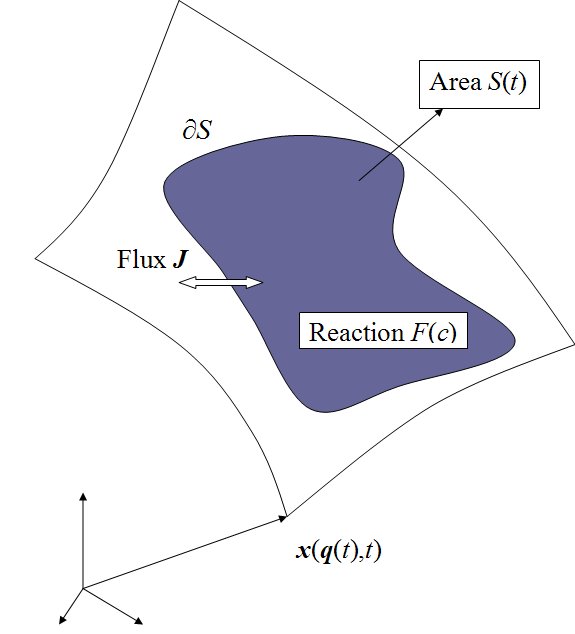
Figure 1: A schematic diagram showing the flux of matter into, and out of a patch of area $S$. This flux comprises advective and diffusive parts, and is given by $\bm{J}=\bm{U}c-\kappa\,\mathrm{grad}c$, and $d\bm{\ell}$ is a line element on the curve formed by the boundary of the area $S$.

of matter created or destroyed by the reaction (shown schematically in Fig. 1), that is,

$$\frac{d}{dt}\int_{S\left(t\right)}c\left(\bm{q},t\right)dS=-\int_{\partial S\left(t\right)}\kappa\,\mathrm{grad}\,c\cdot d\bm{\ell}+\int_{S\left(t\right)}F\left(c\right)dS,$$

where $\kappa$ is the (constant) diffusion coefficient and $\partial S$ is the boundary of $S$. A simple application of Gauss’s law then gives

$$\frac{d}{dt}\int_{S\left(t\right)}c\left(\bm{q},t\right)dS=\int_{S\left(t\right)}\kappa\Delta cdS+\int_{S\left(t\right)}F\left(c\right)dS,\qquad\Delta=\mathrm{div}\,\mathrm{grad}.$$ (2.7)

Combining Eqs. (2.6) and (2.7) gives the following local conservation law:

$$\frac{\partial c}{\partial t}+\mathrm{div}\left(\bm{U}c\right)=\kappa\Delta c+F\left(c\right)-c\frac{\partial\sqrt{|g|}}{\partial t}.$$ (2.8)

The divergence term $\mathrm{div}\left(\bm{U}c\right)$ can be re-written as $U^{i}\partial_{q_{i}}c=\bm{U}\cdot\nabla_{q}c$ for incompressible flows. We call the term $-c\left(\partial\log\sqrt{g}/\partial t\right)$ the geometric sink: its inclusion is necessary to conserve the total number of particles on a time-varying substrate. Note that in previous applications Gjorgjieva2007 ; Plaza2004 the scale function was taken to be a growing function of time, and hence this extra term was indeed a sink; here we consider a general growth function, and thus this term can also act as a source. The geometric source / sink has the following interpretation: given a concentration equation for the number of particles per unit volume, a local source can be introduced in two ways. The first and more obvious way is to inject particles into the system. Here, instead of increasing or decreasing the local number of particles, we stretch or squeeze the local area element, so that the local concentration changes. This effect vanishes upon integration, so that the total number of particles is conserved in a global sense, although locally, the number of particles per unit volume changes because the volume itself changes.

We non-dimensionalize Eq. (2.8) to understand the relative importance of stirring, diffusion and reaction kinetics on the dynamics. Given a characteristic length scale $L$, and a characteristic speed $U$ of an incompressible velocity field $\bm{U}$, Eq. (2.8) is parametrised by the Péclet number $Pe={LU}/{\kappa}$ and the Damköhler number $Da={\sigma L}/{U}$, such that

$$\frac{\partial c}{\partial t}+\mathrm{div}\left(\bm{U}c\right)=Pe^{-1}\Delta c+Da\;c(1-c)-c\frac{\partial\mathrm{log}\sqrt{|g|}}{\partial t};$$ (2.9)

these groups respectively describe the ratio of the advective/diffusive and chemical/advective timescales. For any stirring variation, the group $DaPe=\sigma L^{2}/\kappa=Const.$ is unchanged. Hece for a fixed diffusion coefficient $\kappa$, the chemical timescale $1/\sigma$ is the only free parameter controlling the dynamics. Thus, by keeping the other parameters fixed, the chemical timescale sufficiently represents the dynamical timescale of the reaction-advection-diffusion equation Neufeld2001 . Accordingly, the case of a homogeneous concentration field discussed above (2.3) is equivalent to having a very fast reaction rate with respect to a fixed diffusion of order $O(Pe)=1$ and no advection, i.e. $Da\gg 1$. From now on we shall fix the diffusion rate at order unity and describe the dynamics in similar terminology, such that the reaction takes place at a rate measured against the diffusion rate.

3 Scale separation with stirring and surface modulation

The macroscopic behaviour of a system with phenomena occurring at various length and time scales can be described by homogenization theory. The PDE (and its boundary conditions) that describes the system, is analyzed as having rapidly oscillating differential operators corresponding to the different scales of the phenomena. Taking the appropriate limit of infinite scale separation, the solution of the homogenized PDE (known as the cell problem) describes the large-scale behavior induced by the small-scale dynamics. In this section, we use this approach to calculate the effective diffusivity for the reaction-advection-diffusion equation, for a certain class of substrates. The type of substrate modulation we specify is rather restrictive, although our results will demonstrate the qualitative effects of substrate modulation.

3.1 The uniform solution

If the metric tensor in the reaction-advection-diffusion equation (2.9) satisfies certain restrictions, a homogeneous concentration field $c_{0}(t)$ exists. To see this, we set the operators $\mathrm{div}$ and $\Delta$ to zero in the equation, which gives rise to the following form:

$$\frac{dc_{0}}{dt}=Da\;c_{0}\left(1-c_{0}\right)-c_{0}\frac{\partial\log\sqrt{g}}{\partial t}.$$ (3.1)

If, either

• $\sqrt{|g|}=\rho\left(t\right)G\left(\bm{q}\right)$, or more restrictively,

• $g_{ij}=\rho\left(t\right)G_{ij}\left(\bm{q}\right)$,

then we call the metric tensor separable or fully separable respectively. We call the time-dependant separable term $\rho(t)$ the scale function. Note the following observation:

$$\mathrm{det}({g}_{ij})=\rho G\text{ does not imply that }{g}_{ij}=\rho{G}_{ij}.$$

One example of such non-equality is furnished by the metric of the torus in Eq. (3.14). By choosing an appropriate modulation of the inner and outer toroidal radii, the metric of the torus can, however, be made fully separable. Thus, using a separable metric, we have the equality

$$\frac{\partial\log\sqrt{g}\left(\bm{q},t\right)}{\partial t}=\frac{1}{\rho(t)}\frac{d\rho(t)}{dt}$$ (3.2)

and hence the differential equation for the uniform concentration is itself uniform, and this approach is self-consistent. Restricting to this class of substrate modulation, the homogeneous concentration field has an explicit solution as the solution of a Bernoulli equation Polyanin_odes :

$$c_{0}\left(t\right)=\frac{e^{\int_{0}^{t}(Da-\frac{d\log{\rho}}{dt^{\prime}})dt^{\prime}}}{\frac{1}{c_{0}(0)}+Da\;\int_{0}^{t}\{e^{\int_{0}^{t^{\prime}}(Da-\frac{d\log{\rho}}{dt^{\prime\prime}})dt^{\prime\prime}}\}dt^{\prime}}.$$ (3.3)

In the following applications, we shall make use of the growth function

$$\gamma\left(t\right)=Da\left[t-2\int_{0}^{t}c_{0}\left(s\right)ds\right],$$

which satisfies the following important result:

Proposition 1 (The growth function $\gamma\left(t\right)$ is bounded in time.)

This result holds when the scale function $\rho\left(t\right)$ is bounded below, $0<\rho_{\mathrm{min}}\leq\rho\left(t\right)$. We re-write $c_{0}\left(t\right)$ as a perfect derivative, using the notation $f(t)\mathrel{\raisebox{0.29707pt}{:}\!\!=}\rho^{-1}(t)e^{Da\;t}$

$$c_{0}(t)=\frac{1}{Da}\frac{d\log{(\frac{1}{c_{0}(0)}+Da\int_{0}^{t}f(s)ds)}}{dt},$$

so that its integral is simply

$$\int_{0}^{t}c_{0}(s)ds = \frac{1}{Da}\bigg{\{}\log\left[\frac{1}{c_{0}(0)}+Da\int_{0}^{t}f(s)ds\right]-\log\left(\frac{1}{c_{0}(0)}\right)\bigg{\}},$$

$$= \frac{1}{Da}\log\left[1+Dac_{0}\left(0\right)\int_{0}^{t}f(s)ds\right].$$

Thus,

$$\gamma\left(t\right) = Da\,t-2\log\left[1+Dac_{0}\left(0\right)\int_{0}^{t}f(s)ds\right],$$

$$= 2\bigg{\{}\log\left(e^{{Da\,t}/2}\right)-\log\left[1+Dac_{0}\left(0\right)\int_{0}^{t}f(s)ds\right]\bigg{\}},$$

$$= 2\log\left[\frac{e^{{Da\,t}/2}}{1+Dac_{0}\left(0\right)\int_{0}^{t}f(s)ds}\right],$$

$$\leq 2\log\left[\frac{e^{{Da\,t}/2}}{1+\frac{Dac_{0}\left(0\right)}{\rho_{\mathrm{min}}}\int_{0}^{t}e^{Das}ds}\right],$$

and this last quantity has a $t$-independent upper bound, $\gamma_{0}$.

3.2 The homogenized solution

We homogenize the advection-reaction-diffusion equation on a manifold $\mathcal{M}$. For this approach to work, we must specialize to a manifolds with certain special properties. Because homogenization theory is, in general, applicable only to periodic domains, the surface $\mathcal{M}$ must either be a periodic surface embedded in $\mathbb{R}^{3}$, or the torus $\mathbb{T}^{2}$, with an appropriate modulation of the radii. We make the further restriction that the metric tensor of the manifold $\mathcal{M}$ be fully separable, and that the modulation of the manifold is periodic in time. The separability condition means that the co-ordinates $\bm{q}$ are independent of time. Then, the advection-reaction-diffusion equation, written in co-ordinate form $\bm{q}=\left(q^{1},q^{2}\right)$, is the following:

$$\frac{\partial c}{\partial t}+\frac{1}{\sqrt{|G|}}\frac{\partial}{\partial q^{i}}\left(\sqrt{|G|}U^{i}c\right)=\frac{Pe^{-1}}{\rho\left(t\right)\sqrt{|G|}}\frac{\partial}{\partial q^{i}}\left(\sqrt{|G|}G^{ij}\frac{\partial c}{\partial q^{j}}\right)+F\left(c\right)-c\frac{\partial\log\rho}{\partial t}.$$

Thus, we have isolated the modulation terms, and the equation can be expressed in a form where the differential operators are independent of time:

$$\frac{\partial c}{\partial t}+\mathrm{div}_{0}\left(\bm{U}\left(\bm{x},t\right)c\right)=\frac{\rho\left(0\right)}{\rho\left(t\right)}Pe^{-1}\Delta_{0}c+F\left(c\right)-c\frac{\partial\log\rho}{\partial t},$$ (3.4)

where $\Delta_{0}\phi=\rho\left(0\right)^{-1}|G|^{-1/2}\partial_{q_{i}}\left(|G|^{1/2}G^{ij}\partial_{q_{j}}\phi\right)$. For ease of notation, we absorb the prefactor $\rho\left(0\right)$ into the inverse Péclet number.

Solving the full logistic model (3.4) is problematic, as it is a non-linear equation. Fortunately, it is possible to understand the distribution of spatial variations in detail simply by studying the linearized form

$$c(\bm{q},t)=c_{0}(t)+\delta\psi(\bm{q},t),$$ (3.5)

where $\delta\ll 1$ and the advection only affects the second term, $\psi\left(\bm{q},t\right)$. Then, the reaction-advection-diffusion equation becomes

$$\left(\frac{\partial}{\partial{t}}-Da\left[1-2c_{0}\left(t\right)\right]+\frac{\partial\log\rho}{\partial t}\right)\psi=-\mathrm{div}_{0}\left(\bm{U}\psi\right)+\frac{Pe^{-1}}{\rho\left(t\right)}\Delta_{0}\psi.\qquad$$ (3.6)

This evolution equation provides a uniform bound on $\|\psi\|_{2}^{2}$, and hence the decomposition (3.5) is valid for all times.

Proposition 2 (The quantity $\|\psi\|_{2}$ is uniformly bounded.)

To see this, multiply Eq. (3.6) by $\psi\sqrt{|g|}dq^{1}dq^{2}$ and integrate. Using the incompressibility condition, this gives the equation

$$\frac{d}{dt}\|\psi\|_{2}^{2}=-\frac{Pe^{-1}}{\rho\left(t\right)}\|\mathrm{grad}\psi\|_{2}^{2}+\underbrace{Da\left(1-2c_{0}\left(t\right)\right)}_{=d\gamma\left(t\right)/dt}\|\psi\|_{2}^{2},$$

where

$$\|\psi\|_{2}^{2}=\int_{\Omega_{q}}|\psi|^{2}\sqrt{|g|}dq^{1}dq^{2}.$$

Then,

$$\frac{d}{dt}\left(\|\psi\|_{2}^{2}e^{-\gamma(t)}\right)=-\frac{Pe^{-1}}{\rho\left(t\right)}e^{-\gamma(t)}\|\mathrm{grad}\psi\|_{2}^{2}.$$

Integrating,

$$\rho_{\mathrm{min}}\int|\psi|^{2}\sqrt{|G|}dq^{1}dq^{2}\leq\|\psi\|_{2}^{2}\left(t\right)\leq\|\psi\|_{2}^{2}\left(0\right)e^{\gamma\left(t\right)}\leq\|\psi\|_{2}^{2}\left(0\right)e^{\gamma_{0}},$$

since the growth function $\gamma\left(t\right)$ is bounded. This gives the required result.

Before outlining the homogenization method, we re-work Eq. (3.6) such that we are left with the simplest possible equation. First, by re-defining time, $\tau=\int dt\rho\left(t\right)^{-1}$, the equation to homogenize has time-dependence only in the velocity and reaction terms:

$$\left[\frac{\partial c}{\partial\tau}-s\left(\tau\right)\right]\psi=\left[-\bm{V}\left(\bm{q},\tau\right)\cdot\nabla_{q}+Pe^{-1}\Delta_{0}\right]\psi,$$

where

$$s\left(\tau\right)=Da\rho\left(\tau\right)\left(1-2c_{0}\left(\tau\right)\right)-\frac{d\log\rho}{d\tau},\qquad{V}^{i}=U^{i}\left(\bm{q},\tau\right)\rho\left(\tau\right).$$

The time-dependent source term can be eliminated altogether through the use of the equation

$$\frac{\partial\Psi}{\partial\tau}=\left[-\bm{V}\left(\bm{q},\tau\right)\cdot\nabla_{q}+Pe^{-1}\Delta_{0}\right]\Psi,$$ (3.7)

where

$$\psi=\Psi\left(\bm{q},\tau\right)e^{\int s\left(\tau\right)d\tau}.$$

Note that the transformation $\tau=\int^{t}ds/\rho\left(s\right)$ is well-defined because it is invertible, $d\tau/dt=\rho\left(t\right)^{-1}\geq 0$. We now focus on homogenizing Eq. (3.7)). To do this, we must distinguish the time- and length scales in the problem. We work with a velocity field ${\bm{V}}\left(\bm{q},t\right)$ that varies rapidly in space and time, on scales $\varepsilon$ and $\varepsilon^{2}$, respectively. The parameter $\varepsilon$ is obtained from the ratio $\varepsilon=\ell/L$, where $\varepsilon$ is the correlation length of the velocity field, and $L$ is the domain size. We have chosen the timescale of variation to be $\varepsilon^{2}$ for definiteness, although other, slower and faster, scales are possible. We assume that $\rho\left(t\right)$ is periodic in time and varies on the scale $\varepsilon^{2}$ while and $G_{ij}\left(\bm{q}\right)$ varies only on the small length scale $\varepsilon$, or on the box-size scale, but not on both scales.

The metric has small-scale variations:

We introduce the auxiliary function $\Psi_{\varepsilon}=\Psi\left(\bm{q}/\varepsilon,\tau/\varepsilon^{2}\right)$, which satisfies the equation

$$\frac{\partial\Psi_{\varepsilon}}{\partial\tau}=\left[-\varepsilon^{-1}\bm{V}\left(\bm{q},\tau\right)\cdot\nabla_{q}+Pe^{-1}\Delta_{0}\right]\Psi_{\varepsilon}.$$ (3.8)

Next, we introduce auxiliary independent variables $\bm{Q}=\bm{q}/\varepsilon$ and $\sigma=\tau/\varepsilon^{2}$, such that

$$\nabla = \nabla_{\bm{q}}+\varepsilon^{-1}\nabla_{\bm{Q}}$$

$$\Delta = \Delta_{\bm{q}}+2\varepsilon^{-1}\mathrm{div}_{\bm{Q}}\mathrm{grad}_{\bm{q}}+\varepsilon^{-2}\Delta_{\bm{Q}},$$

while the time derivative now also has two components:

$$\frac{\partial}{\partial\tau}+\varepsilon^{-2}\frac{\partial}{\partial\sigma}.$$

The PDE now reads,

$$\left(\frac{\partial}{\partial\tau}+\varepsilon^{-2}\frac{\partial}{\partial\sigma}\right)\Psi_{\varepsilon}=\left(\varepsilon^{-2}\mathcal{L}_{0}+\varepsilon^{-1}\mathcal{L}_{1}+\mathcal{L}_{2}\right)\Psi_{\varepsilon},$$

where

$$\mathcal{L}_{0} = -V^{i}\left(\bm{Q},\sigma\right)\frac{\partial}{\partial Q^{i}}+Pe^{-1}\Delta_{\bm{Q}},$$

$$\mathcal{L}_{1} = -V^{i}\left(\bm{Q},\sigma\right)\frac{\partial}{\partial q^{i}}+2Pe^{-1}\mathrm{div}_{\bm{Q}}\mathrm{grad}_{\bm{q}},$$

$$\mathcal{L}_{2} = Pe^{-1}\Delta_{\bm{q}}.$$

We expand the function $\Psi_{\varepsilon}$ in powers of $\varepsilon$, as

$$\Psi_{\varepsilon}(\bm{Q},\bm{q},\tau,\sigma)=\Psi_{0}(\bm{Q},\bm{q},\tau,\sigma)+\epsilon\Psi_{1}(\bm{Q},\bm{q},\tau,\sigma)+\epsilon^{2}\Psi_{2}(\bm{Q},\bm{q},\tau,\sigma)+....$$

Equating powers of $\varepsilon$ in the expansion of the equation (3.8), we obtain the following triad of problems:

$$\frac{\partial\Psi_{0}}{\partial\sigma}-\mathcal{L}_{0}\Psi_{0} = 0,$$ (3.9)

$$\frac{\partial\Psi_{1}}{\partial\sigma}-\mathcal{L}_{0}\Psi_{1} = \mathcal{L}_{1}\Psi_{0},$$ (3.10)

$$\frac{\partial\Psi_{2}}{\partial\sigma}+\frac{\partial\Psi_{0}}{\partial\tau}-\mathcal{L}_{0}\Psi_{2} = \left(\mathcal{L}_{1}\Psi_{1}+\mathcal{L}_{2}\Psi_{0}\right).$$ (3.11)

By multiplying Eq. (3.9) by $\sqrt{|G|}\left(\bm{Q}\right)\Psi_{0}\left(\bm{Q},\sigma\right)$ and integrating, we obtain

$$\|\Psi_{0}\|_{2}^{2}\left(\sigma_{0}\right)-\|\Psi_{0}\|_{2}^{2}\left(0\right)=-\int_{0}^{\sigma_{0}}\|\mathrm{grad}_{Q}\Psi_{0}\|_{2}^{2}d\sigma.$$

Thus, if $\Psi_{0}$ is $\sigma_{0}$ periodic, then $\Psi_{0}$ is independent of $\bm{Q}$, and hence, is independent of $\sigma$. In symbols,

$$\Psi_{0}=\Psi_{0}\left(\bm{q},\tau\right).$$

Using this solution, the second equation (3.10) becomes

$$\frac{\partial\Psi_{1}}{\partial\sigma}-\mathcal{L}_{0}\Psi_{1}=-V^{i}\left(\bm{Q},\sigma\right)\frac{\partial\Psi_{0}\left(\bm{q},\tau\right)}{\partial q^{i}}.$$

This is solved by the ansatz

$$\Psi_{1}=\theta^{i}\left(\bm{Q},\sigma\right)\frac{\partial\Psi_{0}}{\partial q^{i}},$$

where $\theta^{i}\left(\bm{Q},\sigma\right)$ solves the cell problem

$$\frac{\partial\theta^{i}}{\partial\sigma}-\mathcal{L}_{0}\theta^{i}=-V^{i},\qquad\int_{0}^{\sigma_{0}}d\sigma\int_{\Omega_{Q}}\theta^{i}\left(\bm{Q},\sigma\right)\sqrt{|G|}dQ^{1}dQ^{2}=0,$$

and where $\theta^{i}\left(\bm{Q},\sigma\right)$ is periodic in $\bm{Q}$ and $\sigma$, with periods $1$ and $\sigma_{0}$. Finally, Eq. (3.11) has a solution provided

$$\int_{0}^{\sigma_{0}}\int_{\Omega_{Q}}\left[-\frac{\partial\Psi_{0}}{\partial\tau}+\mathcal{L}_{1}\Psi_{1}+\mathcal{L}_{2}\Psi_{0}\right]\sqrt{|G|}dQ^{1}dQ^{2}=0,$$

that is, if

$$\frac{\partial\Psi_{0}}{\partial\tau}\left(\tau,\bm{q}\right)=Pe^{-1}\Delta_{q}\Psi_{0}\left(\tau,\bm{q}\right)+\frac{1}{|\Omega_{Q}|\sigma_{0}}\int_{0}^{\sigma_{0}}d\sigma\int_{\Omega_{Q}}\mathcal{L}_{1}\Psi_{1}\sqrt{|G|}dQ^{1}dQ^{2}.$$

The second term can be re-arranged as

$$\frac{1}{|\Omega_{Q}|\sigma_{0}}\int_{0}^{\sigma_{0}}d\sigma\int_{\Omega_{Q}}\sqrt{|G|}\left(\bm{Q}\right)dQ^{1}dQ^{2}\left[-V^{i}\theta^{j}+\frac{2Pe^{-1}}{\sqrt{|G|}}\left(\frac{\partial}{\partial Q^{k}}\left(\sqrt{|G|}G^{ki}\theta^{j}\right)\right)\right]\frac{\partial}{\partial q^{i}}\frac{\partial}{\partial q^{k}}\Psi_{0}\left(\bm{q},\sigma\right)\\ =\frac{1}{|\Omega_{Q}|\sigma_{0}}\int_{0}^{\sigma_{0}}d\sigma\int_{\Omega_{Q}}\sqrt{|G|}\left(\bm{Q}\right)dQ^{1}dQ^{2}\left[-V^{i}\theta^{j}\right]\frac{\partial}{\partial q^{i}}\frac{\partial}{\partial q^{k}}\Psi_{0}\left(\bm{q},\sigma\right)\\ =\mathcal{J}^{ij}\frac{\partial}{\partial q^{i}}\frac{\partial}{\partial q^{j}}\Psi_{0}\left(\bm{q},\tau\right),$$

where the result on the second line is a consequence of incompressibility and the periodic boundary conditions. The homogenization matrix

$$\mathcal{J}^{ij}=\frac{1}{|\Omega_{Q}|\sigma_{0}}\int_{0}^{\sigma_{0}}d\sigma\int_{\Omega_{Q}}\sqrt{|G|}dQ^{1}dQ^{2}\left[-V^{i}\theta^{j}\right]$$

is constant because $\sqrt{|G|}=\sqrt{|G|}\left(\bm{Q}\right)$. At lowest order, the equation for $\Psi_{0}\left(\bm{q},\tau\right)$ is

$$\frac{\partial\Psi_{0}}{\partial\tau} = \left(Pe^{-1}\Delta_{q}+\mathcal{M}^{ij}\frac{\partial}{\partial q^{i}}\frac{\partial}{\partial q^{j}}\right)\Psi_{0},$$ (3.12)

$$= \mathcal{K}\Psi_{0},$$

and thus the full solution (to Eq. (3.6)) $\psi$ has a slowly-varying spatial component, multiplied by a rapidly-varying temporal envelope:

$$\psi\left(\bm{Q},\sigma,\tau\right)=\Psi_{0}\left(\bm{Q},\sigma\right)e^{\int s\left(\tau\right)d\tau}.$$

We note the following result:

Proposition 3 (Regularity of the solution $\Psi_{0}\left(\bm{q},\tau\right)$)

The operator $\mathcal{K}$ is negative in the following sense:

$$\int_{\Omega_{q}}dq^{1}dq^{2}\psi\mathcal{K}\psi\leq 0,$$

for any square-integrable function $\psi$, and hence, the solution $\Psi_{0}$ to the equation (3.12) is uniformly bounded in space and time.

The proof of this statement follows from a straightforward computation based on the $\mathcal{J}$-operator:

$$\int_{\Omega_{q}}dq^{1}dq^{2}\psi\underbrace{\mathcal{J}^{ij}\frac{\partial}{\partial q^{i}}\frac{\partial}{\partial q^{j}}}_{=\mathcal{J}}\psi\\ =-\int_{0}^{\sigma_{0}}\int_{\Omega_{Q}}dQ^{1}dQ^{2}\int_{\Omega_{q}}dq^{1}dq^{2}\sqrt{|G|}\left(\bm{Q}\right)U^{i}\left(\bm{Q}\right)\theta^{j}\left(\bm{Q}\right)\psi\left(\bm{q}\right)\frac{\partial}{\partial q^{i}}\frac{\partial}{\partial q^{j}}\psi\left(\bm{q}\right)\\ =\int_{0}^{\sigma_{0}}\int_{\Omega_{Q}}dQ^{1}dQ^{2}\int_{\Omega_{q}}dq^{1}dq^{2}\sqrt{|G|}\left(\bm{Q}\right)U^{i}\left(\bm{Q}\right)\theta^{j}\left(\bm{Q}\right)w_{i}\left(\bm{q}\right)w_{j}\left(\bm{q}\right),\\ =\int_{0}^{\sigma_{0}}\int_{\Omega_{Q}}dQ^{1}dQ^{2}\int_{\Omega_{q}}dq^{1}dq^{2}\sqrt{|G|}\left(\bm{Q}\right)\left(\bm{U}\cdot\bm{w}\right)\left(\bm{\theta}\cdot\bm{w}\right),$$

where $w_{i}=\partial\psi/\partial q^{i}$. We introduce the quantity $\theta_{w}=\bm{w}\cdot\bm{\theta}$, which satisfies $\left(\partial_{\sigma}-\mathcal{L}_{0}\right)\theta_{w}=-\bm{U}\cdot\bm{w}$. Then,

$$\int_{\Omega_{q}}dq^{1}dq^{2}\psi\mathcal{J}\psi = -\int_{0}^{\sigma_{0}}d\sigma\int_{\Omega_{q}}dq^{1}dq^{2}\int_{\Omega_{Q}}dQ^{1}dQ^{2}\sqrt{|G|}\left(\bm{Q}\right)\left[\frac{\partial}{\partial\sigma}\theta_{w}^{2}-\theta_{w}\mathcal{L}_{0}\theta_{w}\right],$$

$$= -\int_{0}^{\sigma}d\sigma\int_{\Omega_{q}}dq^{1}dq^{2}\|\mathrm{grad}_{Q}\theta_{w}\|_{2}^{2}\leq 0.$$

Since $\Psi_{0}$ is uniformly bounded in space and time ($\tau$), our homogenized solution is bounded, and thus consistent with the boundedness result of Prop. 2, provided

$$e^{\int s\left(\tau\right)d\tau}=e^{\int\left[s\left(t\right)/\rho\left(t\right)\right]dt}$$

is bounded in time. This is certainly the case, since the growth function $\gamma\left(t\right)$ is bounded (Prop. 1).

The metric has domain-scale variations:

As before, the PDE to homogeninze reads:

$$\left(\frac{\partial}{\partial\tau}+\varepsilon^{-2}\frac{\partial}{\partial\sigma}\right)\Psi_{\varepsilon}=\left(\varepsilon^{-2}\mathcal{L}_{0}+\varepsilon^{-1}\mathcal{L}_{1}+\mathcal{L}_{2}\right)\Psi_{\varepsilon},$$

where

$$\mathcal{L}_{0}\phi = -\mathrm{div}_{Q}\left(\bm{V}\left(\bm{Q},\sigma\right)\phi\right)+Pe^{-1}\Delta_{\bm{Q}}\phi,$$

$$\mathcal{L}_{1}\phi = -\mathrm{div}_{q}\left(\bm{V}\left(\bm{Q},\sigma\right)\phi\right)+2Pe^{-1}\mathrm{div}_{\bm{Q}}\mathrm{grad}_{\bm{q}}\phi,$$

$$\mathcal{L}_{2}\phi = Pe^{-1}\Delta_{\bm{q}}\phi.$$

The difference is that now $|G|=|G|\left(\bm{q}\right)$, where $\bm{q}$ is the macroscopic scale. This forces the velocity field $V^{i}$ to have the behaviour $V^{i}\left(\bm{Q},\bm{q},\sigma\right)=\tilde{V}^{i}\left(\bm{Q},\sigma\right)/\sqrt{|G|}\left(\bm{q}\right)$, by incompressibility. The triad of problems (3.9)–(3.11) is unchanged, and the solution to Eq. (3.9) is again a function only of the macroscopic scales:

$$\Psi_{0}=\Psi_{0}\left(\bm{q},\tau\right).$$

Using this solution, the second equation (3.10) becomes

$$\frac{\partial\Psi_{1}}{\partial\sigma}-\mathcal{L}_{0}\Psi_{1} = -\mathrm{div}_{q}\left(\bm{V}\left(\bm{Q},\bm{q},\sigma\right)\Psi_{0}\left(\bm{q},\tau\right)\right)$$

$$= -\frac{\Psi_{0}}{\sqrt{|G|}}\frac{\partial}{\partial q^{i}}\left(\sqrt{|G|}V^{i}\right)-V^{i}\frac{\partial\Psi_{0}}{\partial q^{i}}$$

$$= -\frac{\Psi_{0}}{\sqrt{|G|}}\frac{\partial}{\partial q^{i}}\left(\tilde{V}^{i}\left(\bm{Q},\sigma\right)\right)-\frac{\tilde{V}^{i}}{\sqrt{|G|}}\frac{\partial\Psi_{0}}{\partial q^{i}},$$

$$= -\frac{\tilde{V}^{i}}{\sqrt{|G|}\left(\bm{q}\right)}\frac{\partial\Psi_{0}}{\partial q^{i}}.$$

This is solved by the ansatz

$$\Psi_{1}=\frac{\tilde{\theta^{i}}\left(\bm{Q},\bm{q},\sigma\right)}{\sqrt{|G|}}\frac{\partial\Psi_{0}}{\partial q^{i}},$$

where $\theta^{i}\left(\bm{Q},\bm{q},\sigma\right)$ solves the cell problem

$$\frac{\partial\tilde{\theta}^{i}}{\partial\sigma}-\mathcal{L}_{0}\tilde{\theta}^{i}=-\tilde{V}^{i},\qquad\int_{0}^{\sigma_{0}}d\sigma\int_{\Omega_{Q}}\tilde{\theta}^{i}\left(\bm{Q},\bm{q},\sigma\right)dQ^{1}dQ^{2}=0,$$

that is,

$$\frac{\partial\tilde{\theta}^{i}}{\partial\sigma}+\frac{\tilde{V}^{j}}{\sqrt{|G|}}\frac{\partial\tilde{\theta}^{i}}{\partial Q^{j}}-Pe^{-1}\Delta_{Q}\tilde{\theta}^{i}=-\tilde{V}^{i},\qquad$$

The solution $\tilde{\theta}^{i}$ must also satisfy the periodicity condition in $\bm{Q}$ and $\sigma$, with periods $1$ and $\sigma_{0}$, respectively. Note that the macroscopic variable $\bm{q}$ appears parametrically in the equation for $\tilde{\theta}^{i}$. Finally, Eq. (3.11) has a solution provided

$$\int_{0}^{\sigma_{0}}\int_{\Omega_{Q}}\left[-\frac{\partial\Psi_{0}}{\partial\tau}+\mathcal{L}_{1}\Psi_{1}+\mathcal{L}_{2}\Psi_{0}\right]dQ^{1}dQ^{2}=0,$$

that is, if

$$\frac{\partial\Psi_{0}}{\partial\tau}\left(\tau,\bm{q}\right)=Pe^{-1}\Delta_{q}\Psi_{0}\left(\tau,\bm{q}\right)+\frac{1}{|\Omega_{Q}|\sigma_{0}}\int_{0}^{\sigma_{0}}d\sigma\int_{\Omega_{Q}}\mathcal{L}_{1}\Psi_{1}\left(\bm{q},Qv\right)dQ^{1}dQ^{2}.$$

The second term can be re-arranged as

$$\frac{1}{|\Omega_{Q}|\sigma_{0}}\int_{0}^{\sigma_{0}}d\sigma\int_{\Omega_{Q}}dQ^{1}dQ^{2}\left[-\frac{\tilde{V}^{i}\tilde{\theta}^{j}}{\sqrt{|G|}\left(\bm{q}\right)}\frac{\partial}{\partial q^{i}}\frac{1}{\sqrt{|G|}\left(\bm{q}\right)}\frac{\partial}{\partial q^{j}}\Psi_{0}\left(\bm{q},\sigma\right)-\frac{\tilde{V}^{i}}{\sqrt{|G|}\sqrt{|G|}}\frac{\partial\Psi_{0}}{\partial q^{j}}\frac{\partial\tilde{\theta}^{j}}{\partial q^{i}}\right]\\ +\frac{2Pe^{-1}}{|\Omega_{Q}|\sigma_{0}}\int_{0}^{\sigma_{0}}d\sigma\int_{\Omega_{Q}}dQ^{1}dQ^{2}\frac{\partial}{\partial Q^{i}}G^{ij}\frac{\partial}{\partial q^{j}}\left[\frac{\tilde{\theta}^{\ell}}{\sqrt{|G|}}\frac{\partial\Psi_{0}}{\partial q^{\ell}}\right]\\ =\left[\frac{1}{|\Omega_{Q}|\sigma_{0}}\int_{0}^{\sigma_{0}}d\sigma\int_{\Omega_{Q}}dQ^{1}dQ^{2}\left(-\tilde{V}^{i}\tilde{\theta}^{j}\right)\right]\frac{1}{\sqrt{|G|}\left(\bm{q}\right)}\frac{\partial}{\partial q^{j}}\frac{1}{\sqrt{|G|}\left(\bm{q}\right)}\frac{\partial}{\partial q^{j}}\Psi_{0}\left(\bm{q},\sigma\right)\\ -\frac{1}{|G|}\left[\frac{1}{|\Omega_{Q}|\sigma_{0}}\int_{0}^{\sigma_{0}}d\sigma\int_{\Omega_{Q}}dQ^{1}dQ^{2}\left(\tilde{V}^{i}\frac{\partial\tilde{\theta}^{j}}{\partial q^{i}}\right)\right]\frac{\partial\Psi_{0}}{\partial q^{j}}\\ =\frac{1}{\sqrt{|G|}}\frac{\partial}{\partial q^{i}}\frac{\mathcal{J}^{ij}}{\sqrt{|G|}}\frac{\partial}{\partial q^{j}}\Psi_{0}\left(\bm{q},\sigma\right)$$

where the vanishing of the term on the second line is a consequence of the periodic boundary conditions in $\bm{Q}$. Thus, we have obtained the homogenized matrix

$$\mathcal{J}^{ij}\left(\bm{q}\right)=\frac{1}{|\Omega_{Q}|\sigma_{0}}\int_{0}^{\sigma_{0}}d\sigma\int_{\Omega_{Q}}dQ^{1}dQ^{2}\left[-\tilde{V}^{i}\tilde{\theta}^{j}\left(\bm{Q},\bm{q},\sigma\right)\right],$$

which determines the equation for $\Psi_{0}\left(\bm{q},\tau\right)$:

$$\frac{\partial\Psi_{0}}{\partial\tau} = \left(Pe^{-1}\Delta_{q}+\frac{1}{\sqrt{|G|}}\frac{\partial}{\partial q^{j}}\frac{\mathcal{J}^{ij}}{\sqrt{|G|}}\frac{\partial}{\partial q^{j}}\right)\Psi_{0},$$ (3.13)

$$= \mathcal{K}\Psi_{0}.$$

As before, the full solution (to Eq. (3.6)) $\psi$ has a slowly-varying spatial component, multiplied by a rapidly-varying temporal envelope:

$$\psi\left(\bm{q},\sigma,\tau\right)=\Psi_{0}\left(\bm{q},\tau\right)e^{\int s\left(\tau\right)d\tau},$$

where the temporal envelope can depend on $\sigma$ and $\tau$. The diffusion operator is negative because

$$\int_{\Omega_{q}}\sqrt{|G|}dq^{1}dq^{2}\psi\mathcal{K}\psi\leq 0,$$

for any square-integrable function $\psi$. This can be easily verified by examination of the operator

$$\mathcal{J}=\frac{1}{\sqrt{|G|}}\frac{\partial}{\partial q^{i}}\frac{\mathcal{J}^{ij}}{\sqrt{|G|}}\frac{\partial}{\partial q^{j}},$$

which satisfies the relation

$$\int\sqrt{|G|}dq^{1}dq^{2}\frac{1}{\sqrt{|G|}}\psi\frac{\partial}{\partial q^{i}}\frac{\mathcal{J}^{ij}}{\sqrt{|G|}}\frac{\partial\psi}{\partial q^{j}} = \int dq^{1}dq^{2}\psi\frac{\partial}{\partial q^{i}}\frac{\mathcal{J}^{ij}}{\sqrt{|G|}}\frac{\partial\psi}{\partial q^{j}},$$

$$= -\int dq^{1}dq^{2}\frac{\mathcal{J}^{ij}}{\sqrt{|G|}}\frac{\partial\psi}{\partial q^{j}}\frac{\partial\psi}{\partial q^{j}}.$$

Using the trick demonstrated in Prop. 3, the negativity of $\mathcal{J}$, and hence $\mathcal{K}$ is established, and thus $\Psi_{0}$ is uniformly bounded in space and time ($\tau$ and $t$), consistent with Prop. 2.

In conclusion, we have obtained effective diffusion operators for the concentration $\Psi$ in limits when the substrate variation is either large or small in spatial extent (Eqs. (3.12) and (3.13)). A result for a metric that varies on both scales is also obtainable from a combination of these two approaches, provided the metric is separable, $|G|=G_{1}\left(\bm{q}/\varepsilon\right)G_{2}\left(\bm{q}\right)$. We now turn to the calculation of the diffusion constant for a given manifold.

3.3 Shear flow on a modulating torus

We choose an isotropically time-varying torus as our manifold $\mathcal{M}=\mathbb{T}^{2}$, where both the outer and inner radii vary with time according to the constraint $\frac{R(t)}{r(t)}=a>1$. The strict inequality is to preserve the topological character of the torus as a ring torus, thus preventing any degeneration into a horn- or spindle-like surface. Isotropic motion means that neither one of the toroidal angle coordinates is time-dependant. Moreover, either or both of the toroidal radii can be regarded as controlling the scale function $\rho(t)$. We introduce orthogonal co-ordinates $\vartheta-\varphi$, such that $\bm{x}\cdot\hat{\bm{z}}=r\sin\varphi$, where $\bm{x}$ is the position vector and $\hat{\bm{z}}$ is the constant unit vector in the $z$-direction. Thus, the co-ordinate $\varphi$ describes changes in angle around the minor circle. The line element is then

$$ds^{2}=r^{2}d\vartheta^{2}+\left(R+r\cos\vartheta\right)^{2}d\varphi^{2},$$

and thus the metric is diagonal:

$$g_{ij}=\begin{pmatrix}1&&0&&0\\ 0&&r^{2}&&0\\ 0&&0&&(R+r\cos\vartheta)^{2}\end{pmatrix}.$$ (3.14)

Hence, $\sqrt{g}=r(R+r\cos\vartheta)=r^{2}(a+\cos\vartheta)$. We introduce the scale function:

$$\rho(t):=r(t)^{2}=\frac{R(t)^{2}}{a^{2}}$$ (3.15)

which is determined by the time variation of either radius. Now the Laplacian on a torus takes the form

$$\Delta=\frac{1}{r^{2}}\frac{\partial^{2}}{\partial\vartheta^{2}}+\frac{1}{\left(R+r\cos\vartheta\right)^{2}}\frac{\partial^{2}}{\partial\varphi^{2}}-\frac{\sin\vartheta}{r\left(R+r\cos\vartheta\right)}\frac{\partial}{\partial\vartheta},$$

which after utilizing the relation (3.15) can be simply written as

$$\Delta=\frac{1}{\rho}\Delta_{0}=\frac{1}{\rho}\left[\frac{\partial^{2}}{\partial\vartheta^{2}}+\frac{1}{\left(a+\cos\vartheta\right)^{2}}\frac{\partial^{2}}{\partial\varphi^{2}}-\frac{\sin\vartheta}{a+\cos\vartheta}\frac{\partial}{\partial\vartheta}\right].$$ (3.16)

We choose a simple shear flow that varies on the fast scale $\bm{Q}=\left(\varepsilon\vartheta,\varepsilon\varphi\right)$. Specifically,

$$\bm{V}=\frac{1}{\sqrt{|G|}}\left(0,b\left(Q^{1}\right)\right).$$

The cell problem to solve is thus

$$\frac{\partial\theta^{1}}{\partial\sigma}+\frac{b}{\sqrt{|G|}}\frac{\partial\theta^{1}}{\partial Q^{2}}-Pe^{-1}\Delta_{Q}\theta^{1} = 0,$$

$$\frac{\partial\theta^{2}}{\partial\sigma}+\frac{b}{\sqrt{|G|}}\frac{\partial\theta^{2}}{\partial Q^{2}}-Pe^{-1}\Delta_{Q}\theta^{2} = -b\left(Q^{1}\right).$$

The solution is $\bm{\theta}=\left(0,\theta^{2}\left(Q^{1}\right)\right)$, where

$$-D\frac{d^{2}\theta^{2}}{d\left(Q^{1}\right)^{2}}=b\left(Q^{1}\right).$$

Thus, the matrix $\mathcal{J}^{ij}$ is constant and is equal to

$$\mathcal{J}=\left(\begin{array}[]{cc}0&0\\ 0&\mathcal{J}^{22}\end{array}\right),\qquad\mathcal{J}^{22}=\int_{0}^{1}\left|\frac{d\theta^{2}}{dQ^{1}}\right|^{2}dQ^{1}=Pe\int_{0}^{1}\left|\frac{db}{dQ^{1}}\right|^{2}dQ^{1}$$

Note that only the trivial solution is possible if $b$ is replaced with $\rho\left(\sigma\right)b\left(Q^{2}\right)$: in this case, the time-periodicity forces us to choose the zero-solution, and $\mathcal{J}=0$. For the non-trivial case, the homogenized diffusion equation is

$$\frac{\partial\Psi_{0}}{\partial\tau}=Pe^{-1}\left[\frac{\partial^{2}}{\partial\vartheta^{2}}+\frac{1+Pe\mathcal{J}^{22}}{\left(a+\cos\vartheta\right)^{2}}\frac{\partial^{2}}{\partial\varphi^{2}}-\frac{\sin\vartheta}{a+\cos\vartheta}\frac{\partial}{\partial\vartheta}\right]\Psi_{0},$$

which can be solved using standard techniques for self-adjoint operators on bounded domains.

3.4 The extinction of the catalyst

The reduction of the advection term provides a method for understanding the extinction problem. We want to know under what circumstances a small initial concentration $c\left(\bm{q},0\right)=\delta\psi\left(\bm{q},0\right)$, $\delta\ll 1$ will go extinct. The linearized homogenization theory just developed is appropriate here. The homogenized solution is

$$\psi\left(\bm{q},t\right)=e^{Da\,t}\Psi_{0}\left(\bm{q},t\right),$$

where $\Psi_{0}$ satisfies a diffusion equation

$$\rho\left(t\right)\frac{\partial\Psi_{0}}{\partial t}=Pe^{-1}\mathcal{K}\Psi_{0}.$$

Since $\mathcal{K}$ is negative and the manifold $\mathcal{M}$ is smooth, there is a complete set of eigenfunctions $\{A_{\kappa}\left(\bm{q}\right)\}_{\kappa=0}^{\infty}$, with corresponding eigenvalues $\{-\lambda_{\kappa}^{2}\}_{\kappa=0}^{\infty}$. Thus, the solution is given by the superposition

$$\psi\left(\bm{q},t\right)=\frac{\rho\left(0\right)}{\rho\left(t\right)}\sum_{\kappa=0}^{\infty}C_{\kappa}A_{\kappa}\left(\bm{q}\right)e^{Da\,t-\lambda_{\kappa}^{2}Pe^{-1}\int_{0}^{t}\frac{ds}{\rho\left(s\right)}},$$

where the $C_{\kappa}$’s are constant. For a periodic modulation $\rho_{\mathrm{min}}\leq\rho\left(t\right)\leq\rho_{\mathrm{max}}$, the amplitude decays to zero if

$$\mathrm{min}_{\kappa}\lambda^{2}_{\kappa}>Da\,Pe\left(\frac{\rho_{\mathrm{max}}}{\rho\left(0\right)}\right).$$

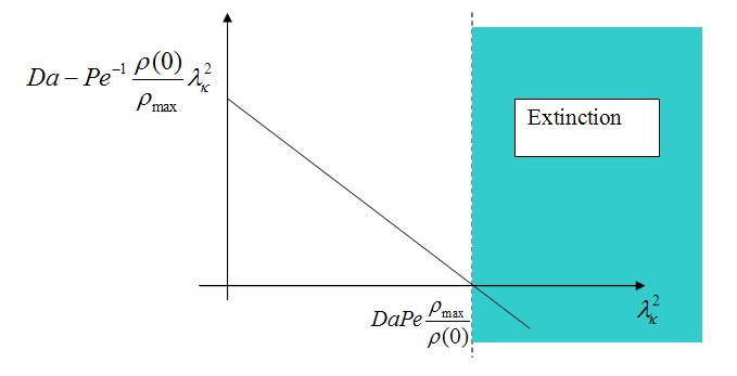
Figure 2: A schematic diagram showing the possibility for the extinction of the catalyst, when $\mathrm{min}_{\kappa}\lambda_{\kappa}^{2}>Da\,Pe\left[\rho_{\mathrm{max}}/\rho\left(0\right)\right]$. The time-varying scale factor $\rho_{\mathrm{max}}\geq\rho\left(0\right)$ shifts the parameter range of extinction to the right, making extinction less likely. On the other hand, the effective diffusion typically shifts the magnitude of the eigenvalues to larger values, thus moving the system further into, or closer to the domain of extinction.

The parameter range of extinction is modified in two ways:

• The factor $\rho_{\mathrm{max}}\geq\rho\left(0\right)$ shifts the extinction threshold to a higher value, as shown in Fig. 2;

• The contribution of the effective diffusion in Eqs. (3.12) and (3.13) is negative in sign, and thus typically increases the magnitude of the eigenvalues $\lambda_{\kappa}^{2}$ relative to the unstirred value. The minimum eigenvalue is then shifted rightward, thus promoting extinction.

Having demonstrated how the full problem can be reduced to a diffusion-type problem in a variety of different situations, we turn our attention to the numerical simulation of reaction-diffusion equations on various surfaces.

4 Numerical case studies

In this section we examine three cases in which substrate modulation affects the reaction propagation. We focus on a modulating torus in three dimensions, where the determinant of the metric tensor is separable, and on a standing-wave substrate in two dimensions, in which case the determinant of the metric tensor is not separable. We also examine the bistable reaction on the torus, in order to verify that our conclusion, namely that appropriate substrate modulation enhances the reaction yield, is independent of the details of the reaction kinetics.

We use both analytical and numerical techniques. Our numerical scheme is a a semi-implicit spectral method in two dimensions. In both situations, the PDE to solve can be written as

$$\frac{\partial c}{\partial t}=\Delta c+\mu,\qquad\mu=\mu\left(\frac{\partial^{2}c}{\partial y^{2}},\frac{\partial c}{\partial x},\frac{\partial c}{\partial y},c,|g|\right).$$ (4.1)

For the torus, we make the identification $x=\theta$, $y=\varphi$, while for the substrate the variables $x$ and $y$ have their usual meaning. We have also scaled all lengths in the problem according to an appropriate length scale $L$, and the time scale is taken to be $L^{2}/D$. For the toroidal case, $L=r_{0}$, a characteristic radius, while for the substrate, $L$ is the periodic box size. Given a time-periodic modulation, there are three non-dimensional frequencies (timescales) in the problem: the diffusive frequency, here normalized to unity, the modulation freqeuncy $\omega$, and the reaction frequency $\tilde{\sigma}=L^{2}\sigma/D$. We are interested in cases where the effects of the chemical reaction and the modulation greatly exceed the diffusive effects, and we therefore take $\omega\approx\tilde{\sigma}\gg 1$. Following standard practice, we henceforth omit ornamentation over non-dimensional quantities. We Fourier-transform the PDE (4.1), which takes the semi-implicit form

$$\frac{\partial c_{\bm{k}}}{\partial t}\left(t_{n}\right)=-\bm{k}^{2}c_{\bm{k}}\left(t_{n+1}\right)+\mu_{\bm{k}}\left(t_{n}\right),\qquad\mu_{\bm{k}}\left(t_{n}\right)=\int_{\left[0,L\right]^{2}}d^{2}\bm{x}e^{-i\bm{k}\cdot\bm{x}}\mu\left[\frac{\partial^{2}c}{\partial y^{2}}\left(\bm{x},t_{n}\right),...\right],$$

which can be integrated forward in time using standard techniques (a similar approach has been used in solving the Cahn–Hilliard equation; see Zhu1999 .) This method relieves the severe constraint on the timestep arising from a fully explicit treatment of the diffusion, and promotes numerical stability. Following standard practice, the discretization in space and time is refined until convergence is achieved.

4.1 A separable modulation on the torus

We use the toroidal co-ordinate system outlined in Sec. 3.3, with the following radial modulation:

$$R(t) = \frac{ar_{0}}{1+\varepsilon\sin\left(\omega t\right)}\qquad 0\leq\varepsilon<1,$$

$$r\left(t\right) = \frac{R\left(t\right)}{a},\qquad a>1,$$ (4.2)

with a magnitude $\varepsilon$ and constant angular frequency $\omega$, which gives the pulsation protocol

$$\rho(t)=\frac{r_{0}^{2}}{\left[1+\varepsilon\sin\left(\omega t\right)\right]^{2}}.$$ (4.3)

It should be noted that the torus, like the sphere, is special in the sense that the scale function, which completely determines the geometric sink, presents itself neatly in the form of the radius. Thus, this case can easily be translated to a time-varying sphere. The protocol (4.3) modifies the yield of the reaction in the homogeneous case. The yield or production is the time-average of the number of molecules created in the reaction, and is defined by writing down the differential number of molecules in a a patch of area

$$dN\left(t\right)=c_{0}\left(t\right)dA\left(t\right).$$

The integral of this quantity is the instantaneous yield:

$$N\left(t\right)=4\pi^{2}a\rho\left(t\right)c_{0}\left(t\right),$$

while the time-average of this quantity is the mean yield:

$$\langle N\rangle=\lim_{t\rightarrow\infty}\frac{1}{T}\int_{0}^{T}N\left(t\right)dt.$$

This mean yield is readily computable in the small-$\varepsilon$ limit. To do this, we use the pulsation relation (4.2), together with the homogeneous solution (3.3), to obtain the asymptotic relation

$$\rho\left(t\right)c_{0}\left(t\right)\sim\\ \frac{r_{0}^{2}}{1+\frac{2\sigma\omega\varepsilon}{\sigma^{2}+\omega^{2}}\left[\frac{\sigma}{\omega}\sin\left(\omega t\right)-\cos\left(\omega t\right)\right]+\tfrac{1}{2}\frac{\varepsilon^{2}}{\sigma^{2}+4\omega^{2}}\left[\sigma^{2}+4\omega^{2}-\sigma^{2}\cos\left(2\omega t\right)-2\omega\sigma\sin\left(2\omega t\right)\right]},\\ \text{as }t\rightarrow\infty.$$ (4.4)

This gives rise to the long-time average

$$\langle N\rangle=4\pi^{2}r_{0}^{2}a\;\lim_{T\rightarrow\infty}\frac{1}{T}\int_{0}^{T}\,N(t)dt,\\ ={4\pi^{2}r_{0}^{2}a}\lim_{T\rightarrow\infty}\frac{1}{T}\int_{0}^{T}\frac{dt}{1+\frac{2\varepsilon\sigma\omega}{\sigma^{2}+\omega^{2}}\left(\frac{\sigma}{\omega}\sin\left(\omega{t}\right)-\cos\left(\omega{t}\right)\right)+\tfrac{1}{2}{\varepsilon^{2}}\left[1-\frac{\sigma^{2}\cos\left(2\omega{t}\right)+2\omega\sigma\sin\left(2\omega{t}\right)}{\sigma^{2}+4\omega^{2}}\right]},\\ =4\pi^{2}r_{0}^{2}a\left[1+\tfrac{1}{2}\varepsilon^{2}\frac{3\sigma^{2}-\omega^{2}}{\sigma^{2}+\omega^{2}}\right]+O\left(\varepsilon^{3}\right),\qquad\omega>0.$$ (4.5)

Thus, the amount of product created can either be raised or lowered, depending on the reaction rate and the pulsation frequency; for large pulsations, the yield is lowered. The exact form of the yield $\langle N\rangle\left(\omega\right)$ is plotted in Fig. 4. Note from this result that $\langle N\rangle\left(\omega\right)$ is not continuous at $\omega=0$. Setting $\omega$ to zero and then averaging gives $\langle N\rangle=4\pi^{2}r_{0}^{2}a$, which is the case of no pulsation. On the other hand, for very slow pulsation (compared to the reaction rate), Eq. (4.5) becomes

$$\langle N\rangle={4\pi^{2}r_{0}^{2}a}\lim_{T\rightarrow\infty}\frac{1}{T}\int_{0}^{T}\frac{dt}{1+2\varepsilon\sin\left(\omega t\right)+\varepsilon^{2}\sin^{2}\left(\omega{t}\right)}={4\pi^{2}r_{0}^{2}a}\left[\frac{\sqrt{1-\varepsilon^{2}}+2\varepsilon^{2}}{1-\varepsilon^{2}}\right].$$ (4.6)

Equation (4.6) is obtained by setting setting the terms in Eq. (4.5) to zero where $\omega$ appears as a factor.

The problem of front propagation on two-dimensional static manifolds has been addressed by Gridndrod and Gomatam Grindrod1987 , and thus some qualitative details of front propagation are available. Such analysis involves the reduction of an equation in the Laplace–Beltrami operator to an associated equation describing front propagation on the line. Since the line is infinite in extent, while the manifold in question is compact, this analysis is valid only for intermediate times, after the front has been established, but before the frontal region experiences the finite extent of the manifold. We apply this technique to the torus by considering an initial disturbance $c\left(\vartheta,\varphi,t=0\right)=c_{0}\left(\vartheta\right)$ centred on $\vartheta=\pi$. This disturbance spreads only in the $\vartheta$ direction. Thus $c\approx 1$ at $\vartheta\approx\pi$, while for early times, the reaction has not propagated around the torus, and $c\approx 0$ at $\vartheta\approx 0$. We denote the location of the front by $\vartheta_{\mathrm{f}}\left(t\right)$, and introduce a moving coordinate $\eta\left(\vartheta,t\right)=\vartheta-\vartheta_{\mathrm{f}}\left(t\right)$, where the function $\vartheta_{\mathrm{f}}\left(t\right)$ is to be determined. The profile of the front is given by a one-dimensional function: $c\left(\vartheta,t\right)=f\left(\eta\right)$, and

$$\frac{\partial{c}}{\partial t}=-f^{\prime}\left(\eta\right)\frac{d\vartheta_{\mathrm{f}}}{dt}.$$

Now for $\eta<0$, $f\approx 1$, while for $\eta>0$, $f\approx 0$. Thus, we are interested in a region $\eta\approx 0$ where the profile of the function $f$ changes rapidly. We therefore write down the Laplacian in the neighbourhood of this point:

$$\Delta c = \frac{\partial^{2}c}{\partial\vartheta^{2}}-\frac{\sin\vartheta}{a+\cos\vartheta}\frac{\partial c}{\partial\vartheta},\qquad a=R/r$$

$$\approx f^{\prime\prime}\left(\eta\right)-\frac{\sin\vartheta_{\mathrm{f}}}{a+\cos\vartheta_{\mathrm{f}}}f^{\prime}\left(\eta\right)+O\left(\eta\right).$$

Putting the reaction-diffusion equation together, we have

$$f^{\prime\prime}\left(\eta\right)+f^{\prime}\left(\eta\right)\left[\frac{d\vartheta_{\mathrm{f}}}{dt}-\frac{\sin\vartheta_{\mathrm{f}}}{a+\cos\vartheta_{\mathrm{f}}}\right]+\sigma f\left(1-f\right)=0.$$

If we stipulate the constant frontal velocity

$$k=\frac{d\vartheta_{\mathrm{f}}}{dt}-\frac{\sin\vartheta_{\mathrm{f}}}{a+\cos\vartheta_{\mathrm{f}}}=\text{Const.},$$ (4.7)

then we are reduced to the reaction-diffusion equation on the line, for the variable $\eta$:

$$f_{\eta\eta}+kf_{\eta}+\sigma f\left(1-f\right)=0.$$

Eq. (4.7) implies that that the velocity of the front is non-constant, and evolves according to the differential equation

$$\frac{d\vartheta_{\mathrm{f}}}{dt}=k+\frac{\sin\vartheta_{\mathrm{f}}}{a+\cos\vartheta_{\mathrm{f}}}.$$ (4.8)

In addition to the constant term $k$, Eq. (4.8) possesses a curvature-related term that can speed up or slow down the front propagation. In particular, there is the possibility of a stationary front when

$$k+\frac{\sin\vartheta_{\mathrm{f}}}{a+\cos\vartheta_{\mathrm{f}}}=0.$$

There is no analogue of the steady-state front in reaction-diffusion on the line. Here it corresponds to a balance between the tendency of the reaction to propagate, and the curvature of the torus, which inhibits the reaction propagation. For moderate to large $\sigma$-values $\sigma=10$–$1000$, the curvature term, being a diffusive contribution, is unimportant relative to the reaction term, and the dynamical equation for $\theta_{\mathrm{f}}$ gives approximately linear growth in time (this is verified by numerical simulation below). Moreover, in this parameter range, it is possible to understand the modulated solution by reference to a flat-space model. Switching on the pulsation clearly will modify the front solution, since the geometric sink $-c\left(\partial\log\sqrt{g}/\partial t\right)=-c\rho^{\prime}\left(t\right)/\rho\left(t\right)$ in the concentration equation breaks the Galilean invariance. However, some quantitative understanding of the front propagation is still possible by studying the small-$\varepsilon$ equation

$$\frac{\partial c}{\partial t}=\left[1+\varepsilon d\left(t\right)\right]^{2}\Delta c+\sigma c\left(1-c\right)-\frac{2\varepsilon cd^{\prime}\left(t\right)}{\left[1+\varepsilon d\left(t\right)\right]^{2}},$$ (4.9)

where

$$\rho=\left[1+\varepsilon d\left(t\right)\right]^{-2},\qquad d\left(t\right)=\sin\left(\omega t\right),$$

and

$$\Delta=\delta^{ij}\frac{\partial}{\partial x^{i}}\frac{\partial}{\partial x^{j}}.$$

Using regular perturbation theory, it can be shown (Appendix A) that the location of the front in this case is given by the formula

$$\vartheta_{\mathrm{f}}\left(t\right)=kt+\varepsilon\left[A\cos\left(\omega t\right)+B\sin\left(\omega t\right)\right]+O\left(\varepsilon^{2}\right),$$

where $A$ and $B$ are amplitudes that are determined from the zeroth and first-order solutions of the equation (4.9), and $kt$ is the reaction front when $\varepsilon=0$. Note that Mendez Mendez2003 tackles a similar problem, but with slowly-varying inhomogeneities and in flat space; the application we have in mind has rapidly-varying temporal co-efficients. Thus, the time-evolution for a periodic geometric sink is a secular drift, coupled with a local-in-time back-and-forth oscillation as the function $\rho\left(t\right)$ is modulated. We can therefore give a qualitative description of the front propagation on the modulating torus: there is a secular drift, which is raised or lowered over the flat case due to curvature effects, while there is a back-and-forth oscillation in the frontal position due to the modulation of the toroidal area. We turn to numerical simulations to check this prediction.

A numerical approach enables us to describe front propagation in the presence of pulsation, and to verify the yield equation (4.5). We work with the pulsation protocol (4.3) and choose a ring-shaped disturbance as an initial condition:

$$c\left(\vartheta,\varphi,t=0\right)=e^{-\left(\vartheta-\pi\right)^{2}/2w^{2}},\qquad w=0.2.$$

Figure 3 shows the front propagation on the pulsating torus. The catalyst is initially centred on $\vartheta=\pi$ and propagates in both directions towards $\vartheta=0$. The concentration of catalyst tends to a uniform amount; however, as the toroidal radii pulsate, the concentration level fluctuates.

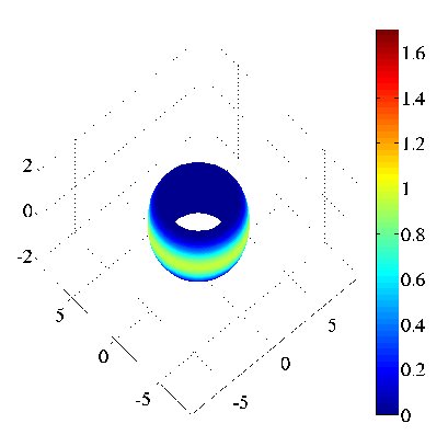
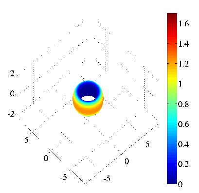
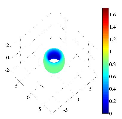
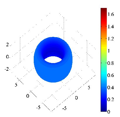
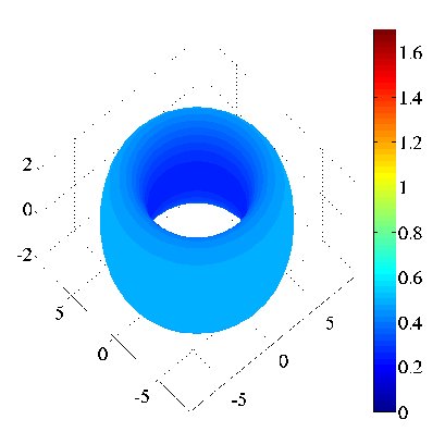
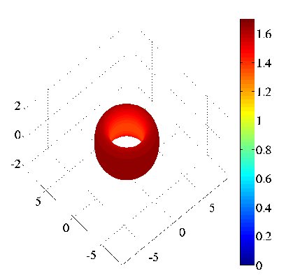
Figure 3: Front propagation on the torus at times $t=0$, $\tfrac{1}{5}T$, $\tfrac{2}{5}T$, $\tfrac{3}{5}T$, $\tfrac{4}{5}T$, $T$, where $T=2\pi/\omega$ is the period of the pulsation. The catalyst is initially centred on $\vartheta=\pi$ and propagates in both directions towards $\vartheta=0$. The concentration of catalyst tends to a uniform amount; however, as the torus radii pulsate, the concentration level fluctuates, as shown in subfigures (d)–(f). We have taken $\omega=\sigma=10$, and $\varepsilon=0.5$.

The most striking effect of the pulsating substrate is seen when the yield of the reaction is studied, as in Fig. 4. The yield fluctuates over time. The maximum yield exceeds the yield in the non-pulsating case, while the minium yield lies below this steady value. Fig. 4 (b) shows the time-average yield as a function of pulsation frequency. There is a discontinuity at $\omega=0$, as discussed in the context of Eqs. (4.5) and (4.6). At slow modulation frequencies, the average yield exceeds that of the non-pulsating case, while for faster modulation frequencies, the average yield decreases relative to this steady value. Fig. 4 (b) also provides a verification of the yield formula Eq. (4.5) and demonstrates the concention that surface modulation can enhance the yield.

Figure 4: (a) The instantaneous yield $\langle N\rangle\left(t\right)$ for $\omega=10=\sigma$, and $\varepsilon=0.5$. The system settles down to a periodic state wherein the concentration fluctuates homogeneously. The dashed line indicates the yield in the absence of pulsation; (b) The time-averaged yield as a function of the pulsation frequency. The graph attains its maximum as $\omega\rightarrow 0$. However, there is a discontinuity at $\omega=0$, and the yield at zero frequency differs from that for very slow pulsations $\omega\rightarrow 0$. This can be seen from Eqs. (4.5) and (4.6) At large values of $\omega$, the yield asymptotes to a constant value. There is excellent agreement between the yield values provided by this graph and the numerical solution of the PDE, and thus, the latter are not shown.

In the absence of pulsation, the speed of the front propagation satisfies Eq. (4.8), as confirmed in Fig. 5 (a). When the pulsation is switched on, there is still a net drift in the location of the front,

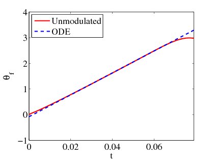
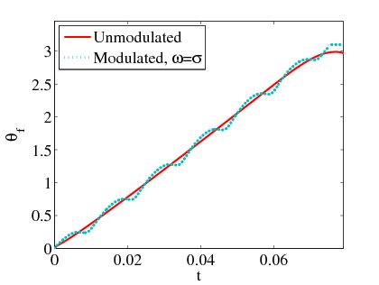
Figure 5: Front propagation on the torus, with $\sigma=500$. Figure (a) shows front propagation on an unmodulated torus, and a comparison with the the front-tracking formula $d\vartheta/dt=k+\left[\sin\vartheta/(a+\cos\vartheta)\right]$, with $k=43$. For large times, the comparison is spoiled since the front wraps around the torus. Subfigure (b) shows the modulated front. The front drifts with the same velocity as in the unmodulated case, while there is a backwards-and-forwards motion as the toroidal area varies periodically.

although locally in time, the front moves forwards and backwards as the surface is modulated. This confirmation of our earlier prediction is shown in Fig. 5 (b). Next, we turn to the study of a qualitatively different case, that of a standing-wave modulation on a substrate, in which case the determinant

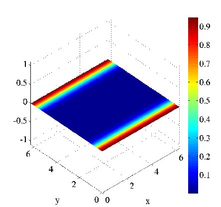
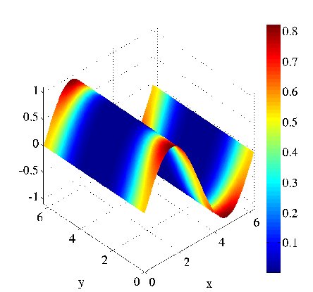
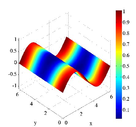
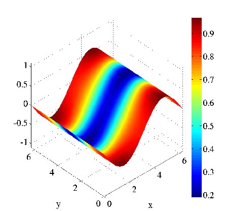
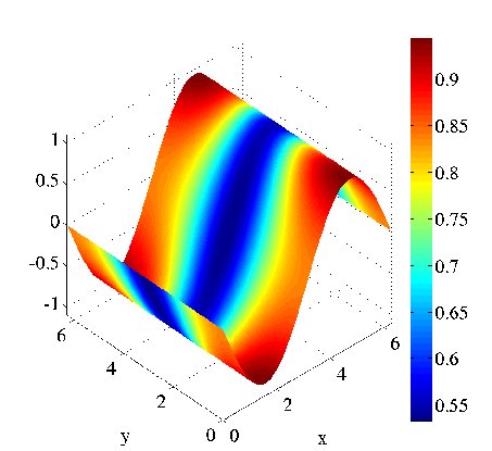
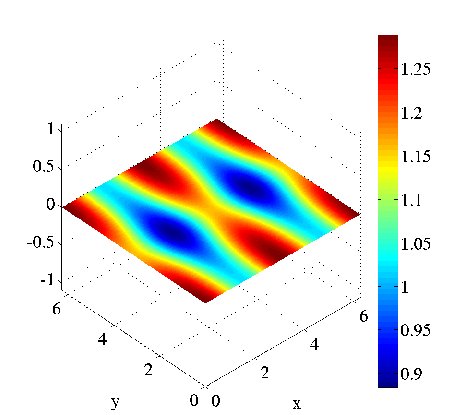
Figure 6: Front propagation on the substrate at times $t=0$, $\tfrac{1}{5}T$, $\tfrac{2}{5}T$, $\tfrac{3}{5}T$, $\tfrac{4}{5}T$, $T$, where $T=2\pi/\omega$ is the period of the pulsation, and $\omega=\sigma=10$. The catalyst is initially centred on $y=0$ and initially in the $y$-direction until a time-periodic state is reached. In reaching this state, the direction of the variation changes, as evidenced by subfigures (e) and (f).

$|g|\left(x,y,t\right)$ is non-separable, and thus the geometric sink depends on space and time.

4.2 A non-seprable modulation: standing wave on a substrate

In this section we work with a general periodic surface embedded in $\mathbb{R}^{3}$ with Cartesian coordinates $\left(x,y,z\right)$. The position vector $\bm{x}$ of a point $P\left(\bm{x}\right)$ on the substrate is given in the Monge parametrization as

$$\bm{x}=\left(x,y,f\left(x,y,t\right)\right),$$

where $f$ is a differentiable function of the planar coordinates $\left(x^{1}=x,x^{2}=y\right)$ and time. The metric tensor is thus

$$\left(g_{ij}\right)=\left(\begin{array}[]{cc}1+f_{x}^{2}&f_{x}f_{y}\\ f_{x}f_{y}&1+f_{y}^{2}\end{array}\right),$$

with inverse

$$\left(g^{ij}\right)=\left(\begin{array}[]{cc}1+f_{y}^{2}&-f_{x}f_{y}\\ -f_{x}f_{y}&1+f_{x}^{2}\end{array}\right).$$

Both of these matrices have determinant

$$|g|=1+f_{x}^{2}+f_{y}^{2}:=1+\left(\nabla_{\perp}f\right)^{2}.$$

For a standing-wave surface

$$f\left(x,y,t\right)=\varepsilon\sin\left(kx\right)\sin\left(\omega t\right),$$

where $k$ and $\omega$ are constants, the Laplacian is

$$\Delta=\frac{\partial^{2}}{\partial{x}^{2}}+\left(1+f_{x}^{2}\right)\frac{\partial^{2}}{\partial{y}^{2}}+\frac{f_{x}f_{xx}}{1+f_{x}^{2}}\frac{\partial}{\partial{x}},$$

that is,

$$\Delta=\frac{\partial^{2}}{\partial{x}^{2}}+\left[1+\varepsilon^{2}k^{2}\cos\left(kx\right)\sin\left(\omega{t}\right)\right]\frac{\partial^{2}}{\partial{y}^{2}}-\frac{\varepsilon^{2}k^{3}\sin\left(kx\right)\cos\left(kx\right)\sin^{2}\left(\omega{t}\right)}{1+\varepsilon^{2}k^{2}\cos^{2}\left(kx\right)\sin^{2}\left(\omega{t}\right)}\frac{\partial}{\partial{x}}.$$

The chemical equation is thus given by

$$\frac{\partial c}{\partial t}=\frac{\partial^{2}c}{\partial{x}^{2}}+\left(1+f_{x}^{2}\right)\frac{\partial^{2}c}{\partial{y}^{2}}+\frac{f_{x}f_{xx}}{1+f_{x}^{2}}\frac{\partial{c}}{\partial{x}}+\sigma\left(c-c^{2}\right)-\frac{2f_{t}f_{xt}}{1+f_{x}^{2}}c$$ (4.10)

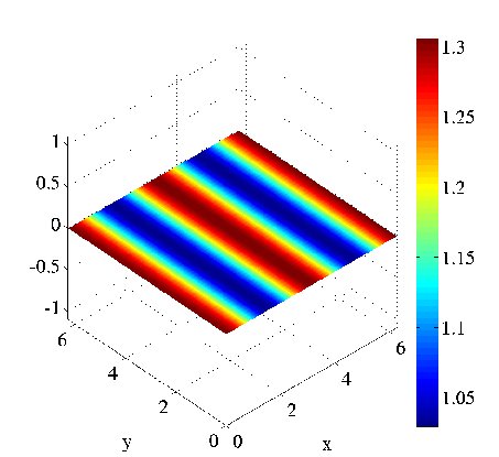
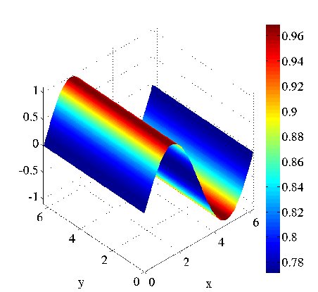
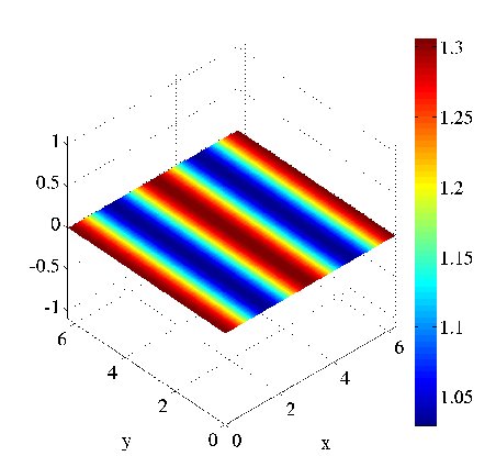
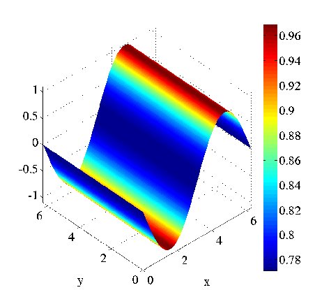
Figure 7: Front propagation on the substrate at times $t=3T$, $\tfrac{13}{4}T$, and $\tfrac{14}{4}T$, and $\tfrac{15}{4}T$, where $T=2\pi/\omega$ is the period of the pulsation, $\omega=\sigma=10$, $k=2\pi/L$, and $\varepsilon=1$. The concentration has reached a time-periodic state where all spatial variations are in the same direction as the direction of the substrate modulation.

Figure 6 shows the case of front propagation for an initial concentration level (Gaussian), with a wavenumber perpendicular to that of the substrate modulation.

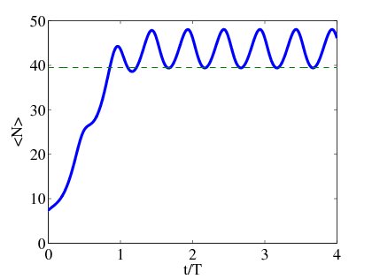
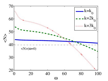
Figure 8: (a) The instantaneous yield $\langle N\rangle\left(t\right)$ for $\omega=10=\sigma$, $k=2\pi/\omega$, and $\varepsilon=1$. This quantity is given by the integral $\int dx\int dy\sqrt{1+f_{x}^{2}}c\left(x,y,t\right)$. The system settles down to a periodic state wherein the concentration flucuates inhomogeneously. The dashed line indicates the yield in the absence of pulsation; (b) The average yield as a function of $\omega$ and wavenumber $k$, where $k_{0}=2\pi/L$ is the fundamental wavenumber. In general, for low pulsation frequencies, the yield is raised relative to the non-modulated case, while for fast frequencies, the yield is lowered. The higher the wavenumber, the stronger the effect.

The front propagates into regions of zero concentration, in an inhomogeneous fashion (since there is spatial modulation in both directions). After about one period of substrate modulation, the spatial variation of the concentration field switches from being in the $y$-direction, to being in the $x$-direction, aligned with the substrate modulation. Eventually, the system attains a time-periodic state, shown in Fig. 7, where the dynamics are driven entirely by the determinantal function $|g|\left(x,t\right)$. On the other hand, for front propagation for an initial disturbance whose wavenumber is parallel to that of the substrate modulation, the f propagates into regions of zero concentration in a homogeneous fashion, and the system rapidly reaches the time-periodic state shown in Fig. 7.

The mean yield is always that associated with with the time-periodic state, since any initial configuration tends asymptotically to this state. The yield function is

$$\langle N\rangle\left(\omega,\varepsilon,k\right)=\bigg{\langle}\int dx\int dy\sqrt{1+f_{x}^{2}}c\left(x,y,t\right)\bigg{\rangle}.$$

We obtain the yield function as a function of the parameters $\omega$, $k$, and $\varepsilon$ by solving Eq. (4.10) numerically in one dimension ($\partial_{y}=0$). The results are shown in Fig. 8. As before, the mean yield as a function of time varies in phase with the substrate modulation, and the maximum mean yield exceeds the stationary case. The time-averaged mean yield depends on the frequency of modulation: the slower the modulation, the greater the yield. Increasing the wavenumber of the modulation enhances this effect, as seen in Fig. 8 (b). In contrast with the toroidal case, the late-time state is not homogeneous, rather it varies periodically in space and time, according to the one-dimensional equation

$$\frac{\partial c}{\partial t}=\frac{\partial^{2}c}{\partial{x}^{2}}+\frac{f_{x}f_{x}^{2}}{1+f_{x}^{2}}\frac{\partial{c}}{\partial{x}}+\sigma\left(c-c^{2}\right)-\frac{2f_{t}f_{xt}}{1+f_{x}^{2}}c.$$

An inhomogeneous final state is undesirable in applications where a pure state involving only the product $B$ is required, and thus a pulsation protocol similar to that on the torus is preferable over the substrate modulation presented here.

4.3 The bistable reaction on the torus

We demonstrate numerically that the reaction yield can be enhanced for other, more complicated mass-action laws, such as the bistable reaction. Here, there are two stable states $c=0$, and $c=1$, and an intermediate, unstable state $c=\alpha_{0}$, where $0<\alpha_{0}<1$. We study this reaction on the pulsating torus; the relevant equation is

$$\frac{\partial c}{\partial t}=\Delta c+\sigma c\left(c-1\right)\left(\alpha_{0}-c\right)-c\frac{\partial\log\sqrt{g}}{\partial t},\qquad\Delta=\frac{1}{\rho}\left[\frac{\partial^{2}}{\partial\vartheta^{2}}+\frac{1}{\left(a+\cos\vartheta\right)^{2}}\frac{\partial^{2}}{\partial\varphi^{2}}-\frac{\sin\vartheta}{a+\cos\vartheta}\frac{\partial}{\partial\vartheta}\right],$$ (4.11)

where $\rho=r\left(t\right)^{2}$; for our pulsation protocol this is $\rho^{-1}=\left[1+\varepsilon\sin\left(\omega t\right)\right]^{2}$.

Using a full two-dimensional numerical simulation, we have verified that an arbitrary initial state tends either to the state $c=0$, or a uniform oscillatory state. The preferred state depends on the pulsation parameters and the unstable level $\alpha_{0}$. To see the relation between these parameters, we studied the uniform equation, obtained by setting $\partial_{\vartheta}=\partial_{\varphi}=0$ in Eq. (4.11). We fixed $\varepsilon=0.5$ and $\sigma=10$ and investigated the state selection as a function of $\omega$ and $\alpha_{0}$. For each value of $\alpha_{0}$ there is a critical frequency such that above that frequency, the zero state is preferred, while below that frequency, an oscillatory state is selected. This relationship is shown in Fig. 9 (a). For large values of $\alpha_{0}$, close to $\alpha_{0}=1$, the critical frequency is shifted downward, indicating that the zero state is preferred for all but the slowest of modulation frequencies. We have investigated the time-averaged mean yield as a function of $\omega$ and fixed $\alpha_{0}$. Fig. 9 (b) shows this relationship for $\alpha_{0}=0.4$. For $\omega<\omega_{\mathrm{c}}\left(\alpha_{0}=0.4\right)$, the time-averaged mean yield exceeds the stationary value (where $\omega=0$), while for $\omega>\omega_{\mathrm{c}}$ the mean yield is zero. This result demonstrates that while more parameter-tuning is required, it is still possible to obtain a yield above the stationary yield simply by an appropriate modulation of the substrate.

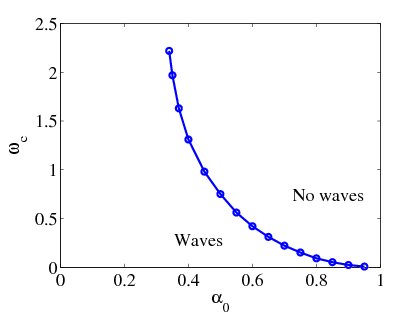
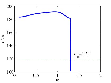
Figure 9: Characterization of the bistable reaction. Subfigure (a) gives the parameter regimes in which either the zero state $c=0$, or the oscillatory state, is selected as the asymptotic state. The oscillatory state is preferred at small frequencies, and the critical frequency is reduced at large $\alpha_{0}$-values. Subfigure (b) gives the time-averaged yield as a function of $\omega$ for $\alpha_{0}=0.4$. The time-averaged yield exceeds the stationary ($\omega=0$; dotted line) yield for $\omega<\omega_{\mathrm{c}}$, while for $\omega>\omega_{\mathrm{c}}$, the yield is zero.

5 Conclusions

We developed a mass-balance law for flow-driven chemical reactions on arbitary, time-varying surfaces. The derivation is quite general, and takes into account situations where the surface co-ordinates are themselves functions of time. Our mass-balance law possesses a geometric source / sink, which modifies the reaction. For isotropic surfaces, where the space- and time-dependence of the metric tensor are separable, this geometric term is a function of time alone, and a homogeneous solution is possible. This solution is explicit for the logistic reaction function, and the dependence of the concentration level on the scale function of the metric tensor is thus made manifest.

In many situations Plaza2004 , the surface of modulation is isotropic, and this case therefore merits close attention. We developed a theory for describing the effects of flow for this class of manifold, and for flow fields with small-scale spatial variations. In such a scenario, homogenization theory permits one to calculate the distribution of concentration through an effective-diffusion equation. Through surface modulation, the effective diffusion coefficient depends on space, although this dependence is eliminated for a class of simple shear flows on the torus; similar results for other surfaces are easily envisioned.

Having demonstrated a method for taking account of flow through the use of an effective diffusivity, we focused on numerical simulations of reaction-diffusion equations. By numerically simulating logistic growth and diffusion on the torus, we demonstrated the existence of reaction fronts that drift at a constant velocity, but periodically advance and recede, due to surface modulation. We also demonstrated that the time-averaged yield of the reaction could be increased by surface modulation. A similar result was found for the bistable growth law, although careful tuning of the modulation frequency in relation to the bistable parameter is necessary for selection of the required asymptotic state. For non-isotropic surfaces, the yield was increased, although a spatially homogeneous state was impossible to attain. In summary, our PDE model and its simplifications provide an insight into the simultaneous processes of chemical reactions, stirring, and surface modulation, and should prove helpful in optimizing the outcome of chemical reactions on variable domains.

Acknowledgements

The authors would like to thank G. Pavliotis for helpful suggestions.

APPENDIX A

In this section we calculate the perturbed speed of front propagation for the following equation in flat space:

$$\frac{\partial c}{\partial t}=\left[1+\varepsilon d\left(t\right)\right]^{2}\Delta c+\sigma c\left(1-c\right)-\frac{2\varepsilon cd^{\prime}\left(t\right)}{\left[1+\varepsilon d\left(t\right)\right]^{2}},$$ (A-1)

where

$$\rho=\left[1+\varepsilon d\left(t\right)\right]^{-2},\qquad d\left(t\right)=\sin\left(\omega t\right),$$

and

$$\Delta=\delta^{ij}\frac{\partial}{\partial x^{i}}\frac{\partial}{\partial x^{j}}.$$

The amplitude $\varepsilon$ is assumed to be small, $\varepsilon\ll 1$. We define the front as the locus of points $x_{\mathrm{f}}\left(t\right)$ in the uni-directional solution $c\left(x,t\right)$, for which

$$c\left(x_{\mathrm{f}}\left(t\right),t\right)=\text{some constant}=C_{0}.$$ (A-2)

When $\varepsilon=0$, the front is located at $x=x_{\mathrm{f}}^{(0)}\left(t\right)=kt$, where $k$ is the constant velocity, which enters into the equation for the front profile:

$$\frac{d^{2}\phi_{0}}{d\eta^{2}}+k\frac{d\phi_{0}}{d\eta}+\sigma\phi_{0}\left(1-\phi_{0}\right),\qquad\eta=x-kt,$$

where $\phi\left(-\infty\right)=0$ and $\phi\left(\infty\right)=1$. We expand the solution to the perturbed problem in powers of $\varepsilon$:

$$c=\underbrace{c_{0}\left(x,t\right)}_{=\phi_{0}\left(\eta\right)}+\varepsilon c_{1}\left(x,t\right)+O\left(\varepsilon^{2}\right).$$

The location of the front must change in order for the constraint (A-2) still to be satisfied:

$$c\left(x_{\mathrm{f}}^{(0)}+\varepsilon x_{\mathrm{f}}^{(1)},t\right)=C_{0}.$$

By Taylor expansion,

$$x_{\mathrm{f}}^{(1)}=-\frac{c_{1}\left(x_{\mathrm{f}}^{(0)},t\right)}{\frac{\partial c_{0}}{\partial x}|_{x_{\mathrm{f}}^{(0)}}}.$$ (A-3)

The first-order equation is

$$\frac{\partial c_{1}}{\partial t}=\Delta c_{1}+\frac{\partial F}{\partial c}\bigg{|}_{c_{0}}c_{1}-2\left[d\left(t\right)\Delta c_{0}+d^{\prime}\left(t\right)c_{0}\right].$$

We introduce new variables $c_{1}=\phi_{1}\left(\eta,t\right)$. Thus,

$$\frac{\partial\phi_{1}}{\partial t} = \mathcal{L}_{\eta}\phi_{1}-2\left[d\left(t\right)\frac{d^{2}\phi_{0}}{d\eta^{2}}+d^{\prime}\left(t\right)\phi_{0}\left(\eta\right)\right],$$

$$= \mathcal{L}_{\eta}\phi_{1}-d\left(t\right)b_{1}\left(\eta\right)-d^{\prime}\left(t\right)b_{2}\left(\eta\right),$$

where

$$\mathcal{L}_{\eta}=\frac{\partial^{2}}{\partial\eta^{2}}+v\frac{\partial}{\partial\eta}+\frac{\partial F}{\partial c}\bigg{|}_{c_{0}\left(\eta\right)}.$$

Since $d$ is periodic, we can write $d=\Re\left(\delta_{0}e^{-i\omega t}\right)$ without loss of generality, and thus $\phi_{1}\left(\eta,t\right)=e^{-i\omega t}\phi_{\omega}\left(\eta\right)$, where $\phi_{\omega}\left(\eta\right)$ satisfies the equation

$$\mathcal{L}_{\eta}\phi_{\omega}=-i\omega\phi_{\omega}+\delta_{0}b_{1}\left(\eta\right)-i\omega\delta_{0}b_{2}\left(\eta\right).$$

Thus,

$$c_{1}\left(x_{\mathrm{f}}^{(0)},t\right)=\phi_{\omega}\left(0\right)e^{-i\omega t}$$

and hence Eq. (A-3) becomes

$$x_{\mathrm{f}}^{(1)}=-\frac{\Re\left(\phi_{\omega}\left(0\right)e^{-i\omega t}\right)}{\phi^{\prime}\left(0\right)}.$$

In other words,

$$x_{\mathrm{f}}\left(t\right)=x_{\mathrm{f}}^{(0)}\left(t\right)+\varepsilon\left[A\cos\left(\omega t\right)+B\sin\left(\omega t\right)\right]+O\left(\varepsilon^{2}\right),$$

where $A$ and $B$ are constants, as claimed in Sec. 4.

References

- (1) S. Strogatz. Nonlinear dynamics and chaos. Perseus, Massachussetts, 1994.
- (2) J. G. Skellam. Random dispersal in theoretical populations. Biometrika, 38:196, 1951.
- (3) J. D. Murray. Mathematical Biology. Springer, Berlin, second edition, 1993.
- (4) S. A. Newman and H. L. Frisch. Dynamics of skeletal pattern formation in developing chick limb. Science, 205:4407, 1979.
- (5) S. Kondon and R. Asal. A reaction-diffusion wave on the skin of the marine angelfish Pomacanthus. Nature, 376:765, 1995.
- (6) E. J. Crampin, E. A. Gaffney, and P. K. Maini. Reaction and diffusion on growing domains: Scenarios for robust pattern formation. Bull. of Math. Biol, 61:1093, 1999.
- (7) J. Gomatam and F. Amdjadi. Reaction-diffusion equations on a sphere: Meandering of spiral waves. Phys. Rev. E, 56:3913, 1997.
- (8) C. Varea, J. L. Aragón, and R. A. Barrio. Turing patterns on a sphere. Phys. Rev. E, 60:4588, 1999.
- (9) M. A. J. Chaplain, M. Ganesh, and I. G. Graham. Spatio-temporal pattern formation on spherical surfaces: Numerical simulation and application to tumour growth. J. Math. Biol., 42:387, 2001.
- (10) R. G. Plaza, F. Sánchez-Garduno, P. Padilla, R. A. Barrio, and P. K. Maini. The effect of growth and curvature on pattern formation. Journal of dynamics and differential equations, 16:1093, 2004.
- (11) J. Gjorgjieva and J. Jacobsen. Turing patterns on growing spheres: The exponential case. Journal of Discrete and Continuous Dynamical Systems, Supplement:436, 2007.
- (12) R. Aris. Vectors, Tensors, and the Basic Equations of Fluid Mechanics. Prentice-Hall, New Jersey, 1962.
- (13) Z. Neufeld. Excitable media in a chaotic flow. Phys. Rev. Lett., 87:108301, 2001.
- (14) Z. Neufeld, C. López, and P. H. Haynes. Smooth-filamental transition of active tracer fields stirred by chaotic advection. Phys. Rev. Lett., 82:2606, 1999.
- (15) S. N. Menon and G. A. Gottwald. On bifurcations in reaction-diffusion systems in chaotic flows. Phys. Rev. E, 71:066201, 2005.
- (16) D. A. Birch, Y.-K. Tsang, and W. R. Young. Bounding biomass in the Fisher equation. Phys. Rev. E, 75:066304, 2007.
- (17) G. Pavliotis and A. M. Stuart. Multiscale Methods. Springer, Berlin, 2008.
- (18) D. W. McLaughlin, G. C. Papanicolaou, and O. R. Pironneau. Convection of microstructure and related problems. SIAM J. Appl. Math., 45:780, 1985.
- (19) P. McCarty and W. Horsthemke. Effective diffusion coefficient for steady two-dimensional convective flow. Phys. Rev. A, 37:2112, 1988.
- (20) S. Rosencrans. Taylor dispersion in curved channels. SIAM J. Appl. Math., 57:1216, 1997.
- (21) George C. Papanicolaou. Diffusion in random media. In Surveys in Applied Mathematics, page 205. Plenum Press, 1995.
- (22) A. Bensoussan, J.-L. Lions, and G. Papanicolaou. Asymptotic analysis for periodic structures. North-Holland, Amsterdam, 1978.
- (23) Z. Neufeld, P. H. Haynes, and Tamás Tél. Chaotic mixing induced transitions in reaction-diffusion systems. Chaos, 12:426, 2002.
- (24) J. Bicak and B. G. Schmidt. Self-gravitating fluid shells and their nonspherical oscillations in Newtonian theory. The Astrophysical Journal, 521:708, 1999.
- (25) D. Hu and P. Zhang. Continuum theory of a moving membrane. Phys. Rev. E, 75:041605, 2007.
- (26) A. D. Polyanin. Handbook of exact solutions for ordinary differential equations. CRC Press, Boca Raton, FL, second edition, 2003.
- (27) J. Zhu, L. Q. Shen, J. Shen, V. Tikare, and A. Onuki. Coarsening kinetics from a variable mobility Cahn–Hilliard equation: Application of a semi-implicit Fourier spectral method. Phys. Rev. E, 60:3564–3572, 1999.
- (28) P. Grindrod and J. Gomatam. The geometry and motion of reaction-diffusion waves on closed two-dimensional manifolds. J. Math. Biol., 25:597, 1987.
- (29) V. Méndez, J. Fort, H. G. Rotstein, and S. Fedotov. Speed of reaction-diffusion fronts in spatially heterogeneous media. Phys. Rev. E, 68:041105, 2003.