Can immobile magnetic vortex nucleate a vortex–antivortex pair?

Abstract

It is shown that under the action of rotating magnetic field an immobile vortex, contrary to a general belief, can nucleate a vortex-antivortex pair and switch its polarity. Two different kinds of OOMMF micromagnetic modeling are used: (i) the original vortex is pinned by the highly–anisotropic easy-axes impurity at the disk center, (ii) the vortex is pinned by artificially fixing the magnetization inside the vortex core in the planar vortex distribution. In both types of simulations a dip creation with a consequent vortex-antivortex pair nucleation is observed. Polarity switching occurs in the former case only. Our analytical approach is based on the transformation to the rotating frame of reference, both in the real space and in the magnetization space, and on the observation that the physical reason for the dip creation is softening of the dipole magnon mode due to magnetic field rotation.

Figure 1: (Color online). The modeling of the vortex–antivortex pair formation for the pinned vortex on the impurity in the Py disk ($300$ nm diameter, $20$ nm thickness, $9$ nm is a diameter of impurity with the easy–axis anisotropy $K=17$ MJ/m³). Snapshots describe the magnetization dynamics at different times under the influence of the rotating in–plane magnetic field ($\omega=6$ GHz, $B=20$ mT). The lower row shows the in–plane magnetization dynamics near the disk center. The in-plane magnetization distribution is indicated by streamlines with arrows. Green and yellow solid lines corresponds to the isosurfaces $m_{x}=0$ and $m_{y}=0$, respectively. The out–of–plane magnetization profiles along the line $\xi$ crossing the impurity is shown above the snapshots (right pictures). Left pictures indicate the in–plane magnetization dynamics in the whole disk.

A magnetic vortex forms a ground state of submicron sized magnetic particles, which provides high density storage and high speed magnetic RAM Cowburn (2002). One bit of information corresponds to the upward or downward magnetization of the vortex core (vortex polarity). Exciting the vortex motion by a high-frequency magnetic fields or by a spin polarized currents, one can switch the vortex polarity on a picoseconds time scale. It is known that the switching process is mediated by a vortex-antivortex pair creation Waeyenberge et al. (2006). Typically to observe this switching phenomenon, one has to excite the low frequency gyroscopical mode, which causes the vortex gyromotion. To the best of our knowledge the vortex core switching was always observed experimentally and by simulations only for a moving vortex. Moreover, there is a strong belief that the switching occurs ‘whenever the velocity of vortex-core motion reaches its critical velocity’ $v_{\text{cri}}$ Lee et al. (2008), which is determined only by the exchange constant $A$; for typical soft materials is about $v_{\text{cri}}\sim 300$ m/s Lee et al. (2008); Vansteenkiste et al. (2008).

In the present Letter we predict the switching for the immobile vortex by a rotating magnetic field. The switching picture also involves the mechanism of a dip formation followed by a nucleation of vortex–antivortex pair. We found that the driving force for the dip formation is the in–plane magnetization inhomogeneity, created by a vortex together with the rotating magnetic field; the vortex out–of–plane structure and the vortex velocity are not principle for this mechanism. These conclusions are confirmed by the micromagnetic simulations and by a simple analytical picture.

Recently, we have reported about the vortex core switching by the homogeneous rotating field $\bm{B}(t)=\left(B\cos\omega t,B\sin\omega t,0\right)$ in the ten GHz range Kravchuk et al. (2007), which is much higher than the gyrofrequency and is in the frequency range of the higher azimuthal mode with $|m|=1$ Ivanov and Zaspel (2005); Zaspel et al. (2005); Zivieri and Nizzoli (2008). Opposite to the pumping with the low gyrofrequency, which results in the visible gyroscopic motion of the vortex position, the high frequency field leads to small amplitude (few nm) oscillations of the vortex position, see the trajectories on Fig. 3 of Ref. Kravchuk et al. (2007). Typical velocities when switching occurs are lower than reported in Ref. Lee et al. (2008). There appears a question: is it necessary for vortex to move in order to switch its polarity?

To achieve switching of the immobile vortex we have performed numerically two different kinds of modeling using OOMMF micromagnetic simulations

(i) We have pinned the vortex by the highly–anisotropic easy-axes impurity at the disk center, see Fig. 1. Since the magnetization is always hold perpendicular to the disk plane within the impurity, shifting of the vortex core from the impurity leads to the increasing of magnetostatic energy of the system. Therefore one can use such type of impurity for pinning of a vortex with out-of-plane core structure in conditions of a weak external influence. Initially, the vortex has a positive polarity $p=+1$. By applying the ac field, which rotates against the vortex polarity, $\omega p<0$ [in a clockwise (CW) direction in our case], one can easily resolve the formation of the dip near the pinned vortex, see Fig. 1(a). Under the action of the field the dip deepens, see Fig. 1(b). When the amplitude of the dip reaches its maximum value, a vortex–antivortex pair is created, see Fig. 1(c). The positions of the vortices and the antivortex can be identified by the cross–section of isosurfaces $m_{x}=0$ and $m_{y}=0$ Hertel and Schneider (2006). One can identify from Fig. 1(c) positions of new born vortex and antivortex as well as the position of the initial vortex, which is (as it is seen from the figure) still at origin. The further dynamics is well known Waeyenberge et al. (2006); Hertel and Schneider (2006); Hertel et al. (2007); Gaididei et al. (2008): the new born antivortex annihilates with pinned original vortex, and eventually only the new born vortex with the opposite polarity survives (see Fig. 1(d)).

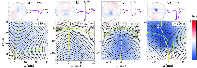
Figure 2: (Color online). The vortex–anivortex pair formation in a Py disk ($150$ nm diameter, $20$ nm thickness) within the fixed core modeling (see the details in the text) under the CW field influence ($\omega=8$ GHz, $B=20$ mT). Notations are the same as on Fig. 1.

(ii) In the second kind of simulations we artificially pinned the vortex core by fixing the magnetization inside the vortex core in the planar vortex distribution, where the normalized magnetization $\bm{m}=\left(\sqrt{1-m_{z}^{2}}\cos\phi;\sqrt{1-m_{z}^{2}}\sin\phi;m_{z}\right)$ takes a form $m_{z}=0$ and $\phi=\chi\pm\pi/2$ with $(r,\chi)$ being the polar coordinates in the disk plane. By this artificially pinned vortex state configuration, the central vortex is a priori immobile, and moreover, without out–of–plane structure. The direction of the dip magnetization is determined only by the direction of the field rotation: if we apply a CCW (CW) field, there appears a dip with $m_{z}>0\,\,(m_{z}<0)$, see Fig. 2. This high frequency field excites also magnon modes. One can resolve the mode with $m=1$ on Figs. 2(a) and (c), and the mode with $m=2$ on Fig. 2(b). During the pumping, the amplitude of the dip increases, and finally, the vortex–antivortex pair is created, see Fig. 2(d). Note that the new–born antivortex can not annihilate with the initial vortex in the fixed core model: it either annihilates with the new born vortex and the scenario repeats again and again, or it stands near the original fixed vortex, while the new born vortex is involved by the field.

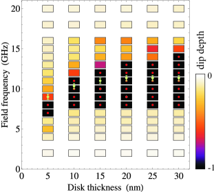
Figure 3: (Color online) Diagram of the frequency range, where the dip formation occurs for a fixed diameter disks ($2R=150$ nm) under the influence of a fixed field amplitude ($B=20$ mT) rotating field. Colors indicate the depth of the dip. The circle over black symbol indicates that the vortex-antivortex pair creation occurs. Light–green symbols indicate frequencies of the azimuthal eigenmode with $m=1$.

The goal of our study is to reveal the mechanism of the dip formation. We follow the simplest model of fixed core planar vortex. Numerically, we found that the dip formation occurs in well defined range of the field parameters $(\omega,B)$, see Fig. 3. When the frequency of the field is less than a critical value $\omega_{c1}$, the dip is not formed. The same happens for the high frequency field ($\omega>\omega_{c2}$). More accurate, out of the borders of the range ($\omega_{c1},\,\omega_{c2}$), the depth of the dip rapidly decreases, what is indicated by colors on Fig. 3. Both critical values $\omega_{c1}$ and $\omega_{c2}$ depend on the disk thickness, which counts in favor of nonlocal magnetostatic nature of this phenomenon. An example of the temporal dependence of the dip depth is plotted on Fig. 4 for a certain disk thickness (15nm), for which $\omega_{c1}$=8GHz and $\omega_{c2}$=12GHz. For $\omega<\omega_{c1}$ just as for $\omega>\omega_{c2}$ the dip depth does not reach its minimal value $m_{z}=-1$, unlike the case $\omega_{c1}<\omega<\omega_{c2}$, when the vortex-antivortex pair is born. The depth of the dip usually makes a number of oscillations while it reaches the limit value. Only for frequencies, which are close to the eigenfrequency of the mode with $|m|=1$, it changes monotonously.

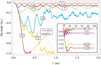
Figure 4: (Color online) Amplitude of $m(t)$ at the minimum (dip center) for the disk($2R=150$ nm, $h=15$ nm) under the influence of rotating field with a fixed amplitude $B=20$ mT and different frequencies. Numbers in rectangle frames denotes frequencies in GHz. The inset contains the time dependence of the dip depth $-\bar{m}(t)$ obtained from the effective Lagrangian (2) for $\omega_{0}=2,\omega_{1}=1,b_{e}=0.1,\eta=0.1,c_{1}=c_{2}=0.25,c_{3}=0.1$. Corresponding frequencies in dimensionless units are shown in oval frames.

The magnetic energy of the system under consideration consists of three terms: $\mathscr{E}=\int\!\mathrm{d}^{3}\bm{r}\left(W_{\text{ex}}+W_{\text{ms}}+W_{\text{f}}\right)$, where $W_{\text{ex}}=\ell^{2}\left(\nabla\bm{m}\right)^{2}$ is the exchange energy density,$W_{\text{ms}}=\frac{1}{8\pi}\int\mathrm{d}^{3}\bm{r}^{\prime}\bigl{(}\bm{m}(\bm{r})\cdot\nabla\bigr{)}\bigl{(}\bm{m}(\bm{r}^{\prime})\cdot\nabla^{\prime}\bigr{)}|\bm{r}-\bm{r}^{\prime}|^{-1}$ is the density of magnetostatic interaction energy. And $W_{\text{f}}=-b\sqrt{1-m_{z}^{2}}\cos(\phi-\omega t)$ is the interaction with a magnetic field $\bm{b}=\left(b\cos\omega t,b\sin\omega t,0\right)$. Here and below normalized quantities are used: $\mathscr{E}=E/(4\pi M_{s}^{2})$, $b=B/(4\pi M_{s})$, $\omega$ and $t$ are measured in units $\Omega$ and $1/\Omega$ respectively, where $\Omega=4\pi\gamma M_{s}$ and $\gamma$ is gyromagnetic ratio. In the no-driving case $b=0$ the magnetic energy $\mathscr{E}$ of cylindrical nanoparticles is invariant under transition into a rotated frame of reference: $\tilde{\chi}=\chi-\alpha$, $\tilde{\phi}(\tilde{\chi})=\phi(\chi)-\alpha$. This means that the quantity $J=M_{z}+L_{z}$ with $M_{z}=\int\!\mathrm{d}^{3}\bm{r}(1-m_{z})$ being the magnetization along the cylindrical axis $z$ and $L_{z}=-\int\!\mathrm{d}^{3}\bm{r}(1-m_{z})\partial_{\chi}\phi$ being the $z$-component of the orbital momentum, is conserved. When the ac field is turned on, the total momentum $J$ is not conserved anymore but its existence allows to obtain that in the rotating frame of reference $\tilde{\chi}=\chi-\omega t$, $\tilde{r}=r$, $\tilde{t}=t$, $\tilde{\phi}(\tilde{\chi})=\phi(\chi=\tilde{\chi}+\omega t)-\omega\tilde{t}$ the magnetic energy is time-independent and has the form

$$\tilde{\mathscr{E}}=\mathscr{E}-\omega J,$$

where the last term represents the rotation energy. The dynamics of the system is governed by the Landau–Lifshitz–Gilbert equations which in the rotating frame of reference have the form

$$\frac{\delta\mathscr{L}}{\delta m_{z}}+\frac{\eta}{1-m_{z}^{2}}\frac{\delta\mathscr{E}}{\delta\tilde{\phi}}=0,\qquad\frac{\delta\mathscr{L}}{\delta\tilde{\phi}}+\eta\,(1-m_{z}^{2})\,\frac{\delta\mathscr{E}}{\delta m_{z}}=0,$$

where $\mathscr{L}=(1+\eta^{2})\int\!\mathrm{d}^{3}x(m_{z}-1)\partial_{t}\tilde{\phi}-\tilde{\mathscr{E}}$ is the Lagrangian and $\eta$ is a damping constant.

To gain some insight how the interaction with the magnetic field (which is static in the rotating frame) together with the rotation provides the dip creation we use the Ansatz

$$\begin{split}m_{z}&=\alpha_{0}(t)f_{0}(r)+\left[\alpha_{1}(t)\cos\chi+\alpha_{-1}(t)\sin\chi\right]f_{1}(r),\\ \phi&=\chi+\frac{\pi}{2}+\beta_{0}(t)g_{0}(r)\\ &+\left[\beta_{1}(t)\cos\chi+\beta_{-1}(t)\sin\chi\right]g_{1}(r),\end{split}$$ (1)

where $\bigl{(}f_{m}(r),g_{m}(r)\bigr{)}e^{im\chi}$ are the magnon eigenfunctions with the eigenfrequencies $\omega_{m}\,(m=0,1)$ on the planar vortex background (see e.g. Ivanov and Zaspel (2002) for general case) and $\alpha_{m},$ and $\beta_{m},$ are time dependent coefficients. Inserting the Ansatz (1) into the Lagrangian $\mathscr{L}$ and carrying out integrations over the spatial coordinates, we get an effective Lagrangian in the form

$$\begin{split}\mathscr{L}^{\text{eff}}&=\sum_{m=0,\pm 1}\Big{(}\alpha_{m}\dot{\beta}_{m}-m\,\omega\,\alpha_{m}\,\beta_{-m}\Big{)}-\mathscr{E}^{\text{eff}},\\ \mathscr{E}^{\text{eff}}&=\frac{1}{2}\sum_{m=0,\pm 1}\,\omega_{|m|}\,\left(\alpha_{m}^{2}+\beta_{m}^{2}\right)-b_{e}\beta_{1}\\ &+c_{0}\,\alpha_{0}^{4}+c_{1}\alpha_{0}\left(\alpha_{1}\beta_{-1}-\alpha_{-1}\beta_{1}\right)+c_{2}\left(\alpha_{1}^{2}+\alpha_{-1}^{2}\right)^{2}\\ &+c_{3}\left(\alpha_{1}^{2}+\alpha_{-1}^{2}\right)\left(\beta_{1}^{2}+\beta_{-1}^{2}\right)+c_{4}\Big{[}\Big{(}\alpha_{1}\beta_{1}+\alpha_{-1}\beta_{-1}\Big{)}^{2}\\ &-\Big{(}\alpha_{-1}\beta_{1}-\alpha_{1}\beta_{-1}\Big{)}^{2}\Big{]}+c_{5}\alpha_{0}^{2}\left(\alpha_{1}^{2}+\alpha_{-1}^{2}\right)\\ &+c_{6}\alpha_{0}^{2}\left(\beta_{1}^{2}+\beta_{-1}^{2}\right)+c_{7}\alpha_{0}\beta_{0}\left(\alpha_{1}\beta_{1}-\alpha_{-1}\beta_{-1}\right)\\ &+c_{8}\beta_{0}^{2}\left(\alpha_{1}^{2}+\alpha_{-1}^{2}\right)+\Big{(}\text{higher order terms}\Big{)}.\end{split}$$ (2)

Here the coefficients $c_{j}$ with $j=\overline{0,\dots,8}$ are due to nonlinear terms in the magnetic energy $\mathscr{E}$ and $b_{e}$ is an effective strength of the magnetic field. Equations of motion for the parameters $\alpha_{m},~{}\beta_{m}$ have the form

$$\dot{\alpha_{m}}=m\,\omega\,\alpha_{-m}-\frac{\partial\mathscr{E}^{\text{eff}}}{\partial\beta_{m}}-\eta\frac{\partial\mathscr{E}^{\text{eff}}}{\partial\alpha_{m}},$$

$$\dot{\beta_{m}}=m\,\omega\,\beta_{-m}+\frac{\partial\mathscr{E}^{\text{eff}}}{\partial\alpha_{m}}-\eta\frac{\partial\mathscr{E}^{\text{eff}}}{\partial\beta_{m}}.$$ (3)

Thus the problem under consideration is reduced to the set of three nonlinearly coupled oscillators. When $\omega\ll\omega_{1}$ the linear terms in Eq. (2) dominate and the out-of-plane component of the magnetization $\bar{m}=\sqrt{\alpha_{0}^{2}+\alpha_{1}^{2}+\alpha_{-1}^{2}}$ is small, see inset in Fig. 4. However, as a result of rotation the magnon frequencies in the rotating frame of reference are shifted, $\tilde{\omega}_{m}=\omega_{m}-m\omega$, and the dipole magnon mode (i.e. the azimuthal mode with $m=1$) becomes soft, which can be identified from Fig. 3. Near the threshold where $\tilde{\omega}_{1}$ is small, the nonlinear terms in the Lagrangian $\mathscr{L}$ become crucial and the system goes to a new regime with the finite value of $\bar{m}$, see the inset in Fig. 4. The appearance of the finite $\bar{m}$ we identify with the dip creation. The dip direction is determined by the product $b_{e}\,\omega$: when $b_{e}\,\omega>0(<0)$ the out–of–plane component of magnetization is negative (positive). This result is in a full agreement with the results of full–scale numerical simulations.

In conclusion, we showed that in the presence of immobile planar vortex the rotating magnetic field produces a vortex-antivortex pair. This process is the most efficient in a finite frequency interval which is determined by the aspect ratio and material properties of the nanoparticle. The physical reason of the dip creation with a consequent vortex-antivortex nucleation is softening the dipole magnon mode and magnetic field induced breaking cylindrical symmetry in the rotating frame of reference. In some respects such softness of modes due to rotation is similar to the problem of instability of BEC under rotation Isoshima and Machida (1999), and to the Zel^′dovich–Starobinsky effect for a rotating black hole Takeuchi et al. (2008). Under the continuous pumping, the soft mode is excited, and the system goes to the nonlinear regime, which results in the dip formation.

The authors thank H. Stoll and B. Van Waeyenberge for helpful discussions. The authors thank the MPI Stuttgart, where part of this work was performed, for kind hospitality and acknowledge the support from Deutsches Zentrum für Luft- und Raumfart e.V., Internationales Büro des BMBF in the frame of a bilateral scientific cooperation between Ukraine and Germany, project No. UKR 08/001.

References

- Cowburn (2002) R. P. Cowburn, J. Magn. Magn. Mater. 242-245, 505 (2002).
- Waeyenberge et al. (2006) V. B. Waeyenberge, A. Puzic, H. Stoll, K. W. Chou, T. Tyliszczak, R. Hertel, M. Fähnle, H. Bruckl, K. Rott, G. Reiss, et al., Nature 444, 461 (2006), ISSN 0028-0836.
- Lee et al. (2008) K.-S. Lee, S.-K. Kim, Y.-S. Yu, Y.-S. Choi, K. Y. Guslienko, H. Jung, and P. Fischer, Phys. Rev. Lett. 101, 267206 (pages 4) (2008).
- Vansteenkiste et al. (2008) A. Vansteenkiste, K. W. Chou, M. Weigand, M. Curcic, V. Sackmann, H. Stoll, T. Tyliszczak, G. Woltersdorf, C. H. Back, G. Schütz, et al., X-ray imaging of the dynamic magnetic vortex core deformation (2008).
- Kravchuk et al. (2007) V. P. Kravchuk, D. D. Sheka, Y. Gaididei, and F. G. Mertens, J. Appl. Phys. 102, 043908 (2007).
- Ivanov and Zaspel (2005) B. A. Ivanov and C. E. Zaspel, Phys. Rev. Lett. 94, 027205 (2005).
- Zaspel et al. (2005) C. E. Zaspel, B. A. Ivanov, J. P. Park, and P. A. Crowell, Phys. Rev. B 72, 024427 (2005).
- Zivieri and Nizzoli (2008) R. Zivieri and F. Nizzoli, Phys. Rev. B 78, 064418 (pages 23) (2008).
- Hertel and Schneider (2006) R. Hertel and C. M. Schneider, Phys. Rev. Lett. 97, 177202 (pages 4) (2006).
- Hertel et al. (2007) R. Hertel, S. Gliga, M. Fähnle, and C. M. Schneider, Phys. Rev. Lett. 98, 117201 (pages 4) (2007).
- Gaididei et al. (2008) Y. B. Gaididei, V. P. Kravchuk, D. D. Sheka, and F. G. Mertens, Low Temperature Physics 34, 528 (2008).
- Ivanov and Zaspel (2002) B. A. Ivanov and C. E. Zaspel, Appl. Phys. Lett. 81, 1261 (2002).
- Isoshima and Machida (1999) T. Isoshima and K. Machida, Phys. Rev. A 60, 3313 (1999).
- Takeuchi et al. (2008) H. Takeuchi, M. Tsubota, and G. Volovik, Journal of Low Temperature Physics 150, 624 (2008).