Open quantum system approach to single-molecule spectroscopy

Abstract

In this paper, single-molecule spectroscopy experiments based on continuous laser excitation are characterized through an open quantum system approach. The evolution of the fluorophore system follows from an effective Hamiltonian microscopic dynamic where its characteristic parameters, i.e., its electric dipole, transition frequency, and Rabi frequency, as well as the quantization of the background electromagnetic field and their mutual interaction, are defined in an extended Hilbert space associated to the different configurational states of the local nano-environment. After tracing out the electromagnetic field and the configurational states, the fluorophore density matrix is written in terms of a Lindblad rate equation. Observables associated to the scattered laser field, like optical spectrum, intensity-intensity correlation, and photon-counting statistics, are obtained from a quantum-electrodynamic calculation also based on the effective microscopic dynamic. In contrast with stochastic models, this approach allows to describe in a unified way both the full quantum nature of the scattered laser field as well as the classical nature of the environment fluctuations. By analyzing different processes such as spectral diffusion, lifetime fluctuations, and light assisted processes, we exemplify the power of the present approach.

I Introduction

In spite that in recent years many different experimental techniques have been established, single molecule spectroscopy (SMS) barkaiChem ; michel ; jung , that is, the study of single nano-objects is predominantly realized by purely optical methods, i.e., by measuring the far-electromagnetic field scattered by the system when it is subjected to laser radiation.

In contrast to standard quantum optical systems breuerbook ; carmichaelbook ; milburn ; scully ; loudon ; yariv , where the reservoir is only defined by the background (free) quantized electromagnetic field, in SMS the supporting nano-environment is highly structured. Its definition and specific properties depend on each experimental setup. In fact, the local environment felt by the fluorophore may involve cryogenic single-molecules tamarat ; donley ; kulzer , molecules at room temperature, either immobilized trautman ; MoernerOrrit or diffusing in solution Elson , the solid state matrix supporting a nanocrystal nirmal ; PMichler ; brokmann ; verberk ; kuno ; potatova ; cichosLaser ; cichos ; vanOrden ; bianco , or single bio-molecules Dickson ; xie ; WEMoerner ; caoYang ; Lu ; SWeiss ; valle . Even more, the proper definition of the background electromagnetic field may be modified because the local surrounding of the system may develop fluctuations in its dielectric properties cichos ; valle .

Each specific environment leads to different underlying physical or chemical processes that in turn modify the emission properties of the fluorophore. In most of the situations, it can be model as a two-level optical transition. The central theoretical problem of SMS is to relate the scattered laser field statistics with the underlying nanoscopic environment dynamic. Due to its complexity, its dynamical influence is usually taken into account by adding random elements to the characteristic parameters of the system barkaiChem ; michel ; jung . For example, spectral diffusion processes are taken into account by adding classical noise fluctuations to the transition frequency of the system, while lifetime fluctuations may be associated to transitions between different conformational (chemical or physical) states of the environment. Stochastic Bloch equations zheng ; he ; FLHBrown ; BarkaiExactMandel , stochastic decay rates wang ; brown , modulated reaction models caoYang ; xieSchenter or stochastic reaction coordinates mukamel are some of the associated theoretical models. On the other hand, radiation patterns whose statistics depend on the external laser power Dickson ; WEMoerner ; hoch ; barbara ; talon ; moerner ; wild ; cichosLaser are modeled by introducing extra states coupled incoherently to the upper level of the system molski .

The previous approaches are well-accepted and standard theoretical tools for modeling SMS experiments. They provide a solid basis for describing different experimental observables, such as those associated to the photon counting statistics. Nevertheless, as the influence of both the background electromagnetic field and the reservoir fluctuations are represented in a unified way by a classical noise, in general it is not clear how to calculate arbitrary observables associated to the scattered laser field. This limitation is evident when considering, for example, the optical or absorption spectrum, which is defined in terms of the scattered field correlations.

The previous drawback or limitation could be surpassed if one is able to describe SMS experiments on the basis of a full open quantum system approach. By an open quantum systems approach we mean: (i) the possibility of describing both the fluorophore system and the reservoir fluctuations through a density matrix operator, whose evolution, i.e., its master equation, can be written and adapted to each specific situation. (ii) Describing the quantum nature of the scattered electromagnetic field through operators and providing a closed solution for their evolution, in such a way that a simple procedure for calculating arbitrary field correlations is established. Then, the calculation of observables like the optical spectrum follows straightforwardly. (iii) Characterizing the photon counting process through a Mandel formula and establishing a manageable analytical tool for the explicit calculation of the photon counting probabilities. The main goal of this paper is to demonstrate that it is possible to build up such kind of powerful and general approach, which not only recovers the predictions of standard approaches, but also allows to characterize, in different situations, arbitrary observables associated to the scattered quantum electromagnetic field.

The scarce application of an open quantum system approach to SMS has a clear origin. Due to the complexity of the underlying nano-environment, a microscopic description, from where to deduce the system density matrix evolution, is lacking. We overcome this difficulty by noting that the noise fluctuations induced by the reservoir barkaiChem ; michel ; jung can be associated to a coarse grained representation of its complex structure vanKampen , allowing us to write microscopic interactions that take into account its leading dynamical effects and at the same time are analytically manageable. From the effective microscopic dynamic the system and reservoir fluctuations result described in terms of a Lindblad rate equation. The theoretical validity of these equations for describing non-Markovian open quantum system dynamics was established in Refs. rate ; breuer . The possibility of establishing a quantum-electrodynamic treatment of SMS experiments also relies on the results of Ref. QRT , where the quantum regression hypothesis was analyzed for Lindblad rate master equations.

We remark that recent author contributions anticipated the possibility of establishing the powerful formalism developed in this paper. In Refs. rapid , it was demonstrated that an anomalous fluorescence blinking phenomenon can be dynamically induced by a complex environment whose action can be described by a direct sum of Markovian sub-reservoirs. In Ref. mandel , for the same situation, observables associated to the photon counting process and a mapping with triplet blinking models barkaiChem ; molski were characterized. In Ref. luzAssisted , we shown that fluorescence blinking patterns whose statistics depend on the external laser power can be model through an underlying tripartite interaction. Both situations lead to quantum master equations that correspond to particular cases of the present general formalism. Since in both cases the calculations relied on specific generalizations of a quantum jump approach plenio , there is not a recipe for calculating the scattered field correlations. The present quantum-electrodynamic treatment also fills up this gap.

The paper is outlined as follows. In Sec. II, the effective Hamiltonian microscopic dynamic that defines the full approach is introduced and the evolution of the fluorophore density matrix is obtained. In Sec. III, observables associated to the scattered laser field are derived from the full microscopic approach. In Sec. IV, the photon counting statistics is characterized through a Mandel formula and a generating function approach cook ; mukamelPRA . In Sec. V, the formalism is exemplified by analyzing different kind of environment fluctuations. Processes like spectral diffusion, lifetime fluctuations, and light assisted processes are explicitly characterized through the scattered field observables. In Sec. VI we give the conclusions.

II Effective Microscopic description and density matrix evolution

The total Hilbert space $\mathcal{H}_{\mathcal{T}}$ associated to a SMS experiment is defined by the external product $\mathcal{H}_{\mathcal{T}}=\mathcal{H}_{\mathcal{S}}\otimes\mathcal{H}_{\mathcal{F}}\otimes\mathcal{H}_{\mathcal{B}},$ where each contribution denotes respectively the Hilbert space of: the fluorophore system, the background electromagnetic field, and the rest of the degrees of freedom that define the local nano-reservoir felt by the system. In general, it is impossible to know the total microscopic dynamic of the reservoir $\mathcal{B}$. In order to bypass this task, following an argument presented by van Kampen vanKampen , we notice that the complexity of the reservoir may admits a simpler general description. Since the nano-reservoir can only be indirectly observed through the fluorophore system, its Hilbert space structure can not be resolved beyond the experimental resolution. Therefore, it is split as $\mathcal{H}_{\mathcal{B}}=\oplus_{R=1}^{R_{\max}}\mathcal{H}_{\mathcal{B}_{R}},$ where each subspace $\mathcal{H}_{\mathcal{B}_{R}}$ is defined by the set of all quantum states that lead to the same system dynamic vanKampen . As the reservoir may be characterized by inordinately dense as well as by discrete manifolds of energy levels, some $\mathcal{H}_{\mathcal{B}_{R}}$ may be of finite dimension.

Clearly, the subspaces $\{\mathcal{H}_{\mathcal{B}_{R}}\}_{R=1}^{R_{max}}$ define the maximal information about the reservoir Hilbert space structure that can be achieved from a SMS experiment. Then, our approach consists in representing the reservoir through a set of coarse grained “configurational macrostates”$\{|R\rangle\}_{R=1}^{R_{\max}}$, $\langle R|R^{\prime}\rangle=\delta_{RR^{\prime}}$, each one being associated to each subspace, and writing the total microscopic dynamic in the effective Hilbert space $\mathcal{H}_{\mathcal{T}}^{eff}=\mathcal{H}_{\mathcal{S}}\otimes\mathcal{H}_{\mathcal{F}}\otimes\mathcal{H}_{\mathcal{U}}.$ The configurational Hilbert space $\mathcal{H}_{\mathcal{U}}$ is expanded by the (unknown) configurational macrostates. The approach is closed after defining both, the field quantization and its interaction with the system in the total effective Hilbert space, and the self-dynamics of the configurational states.

II.1 Electromagnetic field quantization

The classical Maxwell equations landau

$$\mathbf{\bigtriangledown}\cdot\mathbf{D} = 0,\ \ \ \ \ \ \ \mathbf{\bigtriangledown}\times\mathbf{E}=-\frac{1}{c}\frac{\partial\mathbf{B}}{\partial t},$$ (1a)

$$\mathbf{\bigtriangledown}\cdot\mathbf{B} = 0,\ \ \ \ \ \ \ \mathbf{\bigtriangledown}\times\mathbf{H}=+\frac{1}{c}\frac{\partial\mathbf{D}}{\partial t},$$ (1b)

provide the basis for the quantization of the electromagnetic field in a material media loudon ; yariv . The macroscopic field vectors are related by the constitutive relations $$\mathbf{D}=\varepsilon\mathbf{E}, \mathbf{B}=\mu\mathbf{H}, \varepsilon \mu c$$ and where and  are the macroscopic material constants and is the light velocity in free space. For an absorptionless dielectric, the Maxwell equations lead to the classical Hamiltonian field

$$H_{\mathcal{F}}=\frac{1}{8\pi}\int_{V}(\varepsilon|\mathbf{E}|^{2}\mathbf{+}\mu|\mathbf{H}|^{2})dV,$$ (2)

where $V$ is the volume of integration.

The canonical field quantization follows from the expansion of the electric and magnetic field in normal modes and by associating to each component a creation and annihilation photon operator. Here, the domain of quantization $V$ is defined by the local surrounding of the system and not by the full volume of the supporting media. In order to take into account the possible dependence of the local field on the configurational bath states, the macroscopic material constants associated to the volume $V$ are written as operators in $\mathcal{H}_{\mathcal{U}},$

$$\varepsilon=\sum_{R}\varepsilon_{R}\left|R\right\rangle\left\langle R\right|,\ \ \ \ \ \ \ \ \ \ \mu=\sum_{R}\mu_{R}\left|R\right\rangle\left\langle R\right|.$$ (3)

Then, depending on the environment configurational state $\{\left|R\right\rangle\},$ the local field is quantized in a media characterized by the (real) constants $\{\varepsilon_{R},\mu_{R}\}.$ Consistently, as the system have nanoscopic dimensions we assume that these constants, in the local surrounding of the fluorophore $(V),$ do not have any spatial dependence. After standard calculations carmichaelbook , both the electric $\mathbf{E}=\mathbf{E}^{(+)}+\mathbf{E}^{(-)}$ and magnetic $\mathbf{H}=\mathbf{H}^{(+)}+\mathbf{H}^{(-)}$ field operators can be written in terms of positive and negative frequency contributions, each one related to the other by an Hermitian conjugation operation. They read

$$\mathbf{E}^{(+)}\! = \!i\sum_{R}\left|R\right\rangle\left\langle R\right|\sum_{\mathbf{k},\lambda}\!\Big{(}\frac{\hbar\omega_{\mathbf{k}}^{(R)}}{2V\varepsilon_{R}}\Big{)}^{1/2}\!\hat{e}_{\mathbf{k}\lambda}e^{i\mathbf{k\cdot r}}a_{\mathbf{k}\lambda},\ \ \ \ \$$ (4a)

$$\mathbf{H}^{(+)}\! = \!i\sum_{R}\left|R\right\rangle\left\langle R\right|\sum_{\mathbf{k},\lambda}\!\Big{(}\frac{\hbar\omega_{\mathbf{k}}^{(R)}}{2V\mu_{R}}\Big{)}^{1/2}\!\hat{e}_{\mathbf{k}\lambda}^{\prime}e^{i\mathbf{k\cdot r}}a_{\mathbf{k}\lambda}.\ \ \ \$$ (4b)

Here, we assumed that inside the volume $$V [a_{\mathbf{k}\lambda},a_{\mathbf{k}^{\prime}\lambda^{\prime}}^{{\dagger}}]=\delta_{\mathbf{kk}^{\prime}}\delta_{\lambda\lambda^{\prime}}, \mathbf{k} \lambda \hat{e}_{\mathbf{k}\lambda}^{\prime}=(\mathbf{\hat{k}\times}\hat{e}_{\mathbf{k}\lambda}), \mathbf{\hat{k}}\equiv\mathbf{k/|k|}. \mathbf{r}$$ the normal modes can be well approximated by plane waves. As usual, the creation and annihilation operators satisfy the commutation relation where and denote the wave vector and polarization of the quantized mode respectively. In agreement with the transversability of the electromagnetic field, the polarization of the magnetic field reads where denotes the position vector. The dispersion relation associated to each configurational state is

$$\omega_{\mathbf{k}}^{(R)}=\frac{c}{\sqrt{\varepsilon_{R}\mu_{R}}}|\mathbf{k}|.$$ (5)

From now on, we take $\mu_{R}\rightarrow 1.$ As is well known landau , this assumption is always valid in an optical regime.

II.2 System and field Hamiltonians

The fluorophore system is defined by a two-level optical transition with natural frequency $\omega_{A}.$ The upper and lower states are denoted as $\left|b\right\rangle$ and $\left|a\right\rangle$ respectively. We take into account that, depending on the configurational state $\left|R\right\rangle,$ the natural frequency $\omega_{A}$ may be shifted a quantity $\delta\omega_{A}^{(R)}.$ These parameters define the spectral shift of the system associated to each state of the reservoir barkaiChem . Therefore, the system and field Hamiltonians are written as

$$H_{\mathcal{S}}=\hbar\omega_{0}\sigma_{z}/2,\ \ \ \ \ \ \ \ H_{\mathcal{F}}=\sum\nolimits_{\mathbf{k}\lambda}\hbar\omega_{\mathbf{k}\lambda}a_{\mathbf{k}\lambda}^{{\dagger}}a_{\mathbf{k}\lambda},$$ (6)

where $H_{\mathcal{F}}$ follows from Eqs. (4) and (2). $\sigma_{z}$ is the z-Pauli matrix written in the base $\{\left|a\right\rangle,\left|b\right\rangle\}.$ The frequency operator of the system is defined by

$$\omega_{0}=\omega_{A}+\sum_{R}\delta\omega_{A}^{(R)}\left|R\right\rangle\left\langle R\right|,$$ (7)

while for the field it reads

$$\omega_{\mathbf{k}\lambda}=\sum_{R}\omega_{\mathbf{k}\lambda}^{(R)}\left|R\right\rangle\left\langle R\right|.$$ (8)

The frequencies $\omega_{\mathbf{k}\lambda}^{(R)}$ are defined by the dispersion relations Eq. (5).

II.3 Dipole-field interaction

The natural decay of the fluorophore is induced by the coupling of its electric dipole with the quantized electric field. Their interaction can be written as

$$H_{\mathrm{dip}}=-\mathbf{E}_{\mathbf{r}_{\mathbf{A}}}\cdot\mathbf{d}_{\mathbf{A}},$$ (9)

where $\mathbf{d}_{\mathbf{E}}$ is the (electric) dipole operator associated to the optical transition and $\mathbf{E}_{\mathbf{r}_{\mathbf{A}}}$ is the electric field operator at the position $\mathbf{r}_{\mathbf{A}}$ of the system. To take into account the different configurational states of the reservoir, the standard definition of the dipole operator $\mathbf{d}_{\mathbf{A}}$ carmichaelbook  is generalized as

$$\mathbf{d}_{\mathbf{A}}=\sum_{R,R^{\prime}}\mathbf{d}_{RR^{\prime}}(\sigma^{{\dagger}}\left|R\right\rangle\left\langle R^{\prime}\right|+\sigma\left|R^{\prime}\right\rangle\left\langle R\right|),$$ (10)

where $\{\mathbf{d}_{RR^{\prime}}\}$ are vectors (assumed real) with units of electric dipole. $\sigma^{{\dagger}}$ and $\sigma$ are respectively the raising and lowering operators acting on the states $\{\left|a\right\rangle,\left|b\right\rangle\}.$ The diagonal contributions $\mathbf{d}_{RR}$ define the dipole associated to each configurational state. The nondiagonal contributions, $\mathbf{d}_{RR^{\prime}}$ with $R\neq R^{\prime},$ take into account the possibility of coupling different configurational states (those of finite dimension) through system transitions.

The dipole-field interaction Eq. (9), in a rotating wave approximation carmichaelbook ; loudon ; milburn ; scully , from Eqs. (4) and (10) reads

$$H_{\mathrm{dip}}=\sum_{\begin{subarray}{c}\mathbf{k},\lambda\\ R,R^{\prime}\end{subarray}}(\kappa_{RR^{\prime}}^{\mathbf{k},\lambda}\sigma^{{\dagger}}\left|R\right\rangle\left\langle R^{\prime}\right|a_{\mathbf{k}\lambda}+\kappa_{RR^{\prime}}^{\mathbf{k},\lambda^{\ast}}\sigma\left|R^{\prime}\right\rangle\left\langle R\right|a_{\mathbf{k}\lambda}^{{\dagger}}),$$ (11)

where the interaction parameters are defined by

$$\kappa_{RR^{\prime}}^{\mathbf{k},\lambda}=-i\Big{(}\frac{\hbar\omega_{\mathbf{k}}^{(R)}}{2V\varepsilon_{R}}\Big{)}^{1/2}e^{i\mathbf{k\cdot\mathbf{r}_{A}}}(\hat{e}_{\mathbf{k}\lambda}\cdot\mathbf{d}_{RR^{\prime}}).$$ (12)

II.4 Environment configurational fluctuations

The previous definitions effectively take into account the influence of the different configurational states of the environment on the fluorophore and the background electromagnetic field as well as into their mutual interaction. Now, in agreement with the van Kampen argument vanKampen , and consistently with real specific situations barkaiChem ; michel ; jung , where the properties of the nano-environment fluctuates in time, the configurational states (associated to dense bath manifolds) must be endowed with a mechanism able to induce transitions between them. We remark that the results developed in Refs. rapid ; mandel ; luzAssisted do not take into account neither rely on this extra dynamical effect, which in the context of an open quantum system approach can only be recover with the present treatment.

In order to maintain a full microscopic description of the effective dynamics, here the (incoherent) transitions $\left|R\right\rangle\leftrightarrow\left|R^{\prime}\right\rangle$ are introduced through the Hamiltonian

$$H_{\mathcal{U}}^{\prime}=H_{\mathcal{U}}+H_{\mathcal{W}}+H_{\mathcal{UW}}.$$ (13)

$H_{\mathcal{U}}$ is the free Hamiltonian of $\mathcal{U},$ $H_{\mathcal{W}}$ define an environment ($\mathcal{W}$) responsible for the transitions $\left|R\right\rangle\leftrightarrow\left|R^{\prime}\right\rangle,$ while $H_{\mathcal{UW}}$ defines their mutual interaction. We assume that the states $\{\left|R\right\rangle\}$ are the eigenvalues of $H_{\mathcal{U}}$ with eigenvalues $\hbar\omega_{R},$ and $\mathcal{W}$ is defined by a continuous set of arbitrary bosonic normal modes

$$H_{\mathcal{U}}=\sum\nolimits_{R}\hbar\omega_{R}\left|R\right\rangle\left\langle R\right|,\ \ \ \ \ \ \ H_{\mathcal{W}}=\sum\nolimits_{j}\hbar\omega_{j}b_{j}^{{\dagger}}b_{j}.$$ (14)

$b_{j}^{{\dagger}}$ and $b_{j}$ are the  creation and annihilation operators of $\mathcal{W}$ respectively. The Hamiltonian $H_{\mathcal{UW}}$ reads

$$H_{\mathcal{UW}}=\hbar\sum\limits_{\begin{subarray}{c}j,R,R^{\prime}\\ R\neq R^{\prime}\end{subarray}}(\chi_{RR^{\prime}}^{j}\left|R\right\rangle\left\langle R^{\prime}\right|b_{j}+\chi_{RR^{\prime}}^{j^{\ast}}\left|R^{\prime}\right\rangle\left\langle R\right|b_{j}^{{\dagger}}).$$ (15)

Then, the transitions $\left|R\right\rangle\leftrightarrow\left|R^{\prime}\right\rangle$ are assisted by the creation or destruction of bosonic excitations in each of the modes of frequency $\omega_{j}.$

II.5 System density matrix evolution

The previous analysis allow to define the unitary dynamic, $(d/dt)\rho_{\mathcal{T}}(t)=-(i/\hbar)[H_{\mathcal{T}},\rho_{\mathcal{T}}(t)],$ of the density matrix $\rho_{\mathcal{T}}(t)$ associated to the Hilbert space $\mathcal{H}_{\mathcal{T}}^{eff}=\mathcal{H}_{\mathcal{S}}\otimes\mathcal{H}_{\mathcal{F}}\otimes\mathcal{H}_{\mathcal{U}}.$ The total Hamiltonian read

$$H_{\mathcal{T}}=H_{\mathcal{S}}+H_{\mathcal{U}}^{\prime}+H_{\mathcal{F}}+H_{\mathrm{dip}},$$ (16)

where each contribution follows from Eqs. (6), (11) and (13). $\rho_{\mathcal{T}}(t)$ describe the statistical dynamical behavior of the system, the electromagnetic field, and the configurational states. The joint dynamic of the fluorophore and the configurational states is encoded in the density matrix $\rho_{\mathcal{SU}}(t),$ which follows after tracing out the degrees of freedom of the background electromagnetic field $\mathcal{F}$ and the reservoir $\mathcal{W},$ i.e., $\rho_{\mathcal{SU}}(t)=\mathrm{Tr}_{\mathcal{FW}}[\rho_{\mathcal{T}}(t)].$ The system density matrix $\rho_{\mathcal{S}}(t)=\mathrm{Tr}_{\mathcal{U}}[\rho_{\mathcal{SU}}(t)],$ can always be written as

$$\rho_{\mathcal{S}}(t)=\sum\nolimits_{R}\rho_{R}(t),$$ (17)

where the base $\{\left|R\right\rangle\}$ was used for taking the trace over $\mathcal{U}.$ The auxiliary states $\rho_{R}(t)\equiv\left\langle R\right|\rho_{\mathcal{SU}}(t)\left|R\right\rangle,$ define the system dynamic “given” that the reservoir is in the configurational state $\left|R\right\rangle.$ The dynamic of the configurational states follows from the populations

$$P_{R}(t)=\mathrm{Tr}_{\mathcal{S}}[\rho_{R}(t)],$$ (18)

which provide the probability that the reservoir is in the configurational state $\left|R\right\rangle$ at time $t.$ Therefore, these objects encode the statistical properties of the noise fluctuations introduced in standard stochastic approaches barkaiChem ; michel ; jung . The expression Eq. (18) follows straightforwardly from the definition $P_{R}(t)\equiv\left\langle R\right|\rho_{\mathcal{U}}(t)\left|R\right\rangle,$ where $\rho_{\mathcal{U}}(t)=\mathrm{Tr}_{\mathcal{S}}[\rho_{\mathcal{SU}}(t)].$

Both, the electromagnetic field $\mathcal{F}$ and the bath $\mathcal{W}$ are assumed to be Markovian reservoirs. Then, their influence can be described through a standard Born-Markov approximation. After some algebra carmichaelbook , the evolution of each state $\rho_{R}(t)$ can be written as a Lindblad rate equation rate ; breuer

$$\dfrac{d\rho_{R}(t)}{dt}\!\! = \!\!\dfrac{-i}{\hbar}[H_{R},\rho_{R}(t)]-\gamma_{R}(\{D,\rho_{R}(t)\}_{+}-\mathcal{J}[\rho_{R}(t)])$$

$$\!\!-\sum\limits_{R^{\prime}}\phi_{R^{\prime}R}\rho_{R}(t)+\sum\limits_{R^{\prime}}\phi_{RR^{\prime}}\rho_{R^{\prime}}(t)$$

$$\!\!-\sum\limits_{R^{\prime}}\gamma_{R^{\prime}R}\{D,\rho_{R}(t)\}_{+}+\sum\limits_{R^{\prime}}\gamma_{RR^{\prime}}\mathcal{J}[\rho_{R^{\prime}}(t)],$$

where $\{\cdots\}_{+}$ denotes an anticonmutation operation. The Hamiltonian reads

$$H_{R}=\frac{\hbar\omega_{R}}{2}\sigma_{z},\ \ \ \ \ \ \ \ \ \ \ \ \omega_{R}=\omega_{A}+\delta\omega_{A}^{(R)},$$ (20)

and the remaining system operators are defined by

$$D=\sigma^{\dagger}\sigma/2,\ \ \ \ \ \ \ \ \ \ \ \ \ \mathcal{J}[\bullet]=\sigma\bullet\sigma^{\dagger}.$$ (21)

The rates associated to the reservoir $\mathcal{W}$ are given by

$$\phi_{RR^{\prime}}=\pi g_{\mathcal{W}}(\Delta_{RR^{\prime}})|\chi_{RR^{\prime}}^{\Delta_{RR^{\prime}}}|^{2}.$$

Here, $g_{\mathcal{W}}(\omega)$ is the density of states of $\mathcal{W}$ and $\Delta_{RR^{\prime}}\equiv\omega_{R}-\omega_{R^{\prime}}$ are the transition frequencies of $\mathcal{U}.$ The rates associated to the field $\mathcal{F}$ read ($\gamma_{R}=\gamma_{RR}$)

$$\gamma_{RR^{\prime}}=2\pi\sum_{\lambda}\int\mathbf{dk}g_{\mathcal{F}}^{(R^{\prime})}(\mathbf{k})|\kappa_{RR^{\prime}}^{\mathbf{k},\lambda}|^{2}\delta(|\mathbf{k}|c-\omega_{A}).$$ (22)

Here, $g_{\mathcal{F}}^{(R)}(\mathbf{k})$ is the density of states of the quantized electromagnetic field associated to each configurational state. By writing

$$g_{\mathcal{F}}^{(R)}(\mathbf{k})\mathbf{dk}=\frac{\omega^{2}V\varepsilon_{R}^{3/2}}{2\pi^{2}c^{3}}d\omega d\Omega,$$ (23)

where $d\Omega$ is the solid angle differential and the contribution $\varepsilon_{R}^{3/2}$ follows from the dispersion relation Eq. (5), after a standard integration carmichaelbook it follows

$$\gamma_{R}=\frac{1}{4\pi}\frac{4\omega_{A}^{3}}{3\hbar c^{3}}|d_{RR}|^{2}\varepsilon_{R}^{1/2},\ \ \ \ \ \ \ \gamma_{RR^{\prime}}=\frac{1}{4\pi}\frac{4\omega_{A}^{3}}{3\hbar c^{3}}|d_{RR^{\prime}}|^{2}\varepsilon_{R^{\prime}}^{1/2}.$$ (24)

For simplicity, it was assumed that the dipole vector $\mathbf{d}_{RR^{\prime}}$ [defined by Eq. (10)] can be written as $\mathbf{d}_{RR^{\prime}}=d_{RR^{\prime}}\mathbf{\hat{d}},$ where $d_{RR^{\prime}}$ is the modulus of the dipole vectors, and the unit vector $\mathbf{\hat{d}}$ does not depend on the coefficient $R$ and $R^{\prime}.$ While this simplification forbid us to analyze the angular dependence of the scattered radiation, the general case can be easily worked out from the present treatment.

The previous expressions rely on the condition $\Delta_{RR^{\prime}}\ll\omega_{A},$ i.e., the transition frequencies of $\mathcal{U}$ are much smaller than the optical frequency $\omega_{A}.$ To simplify the analysis, in Eq. (II.5) we have discarded any shift Hamiltonian contribution induced by the microscopic dynamic. Furthermore, since the fluorophore $\mathcal{S}$ is an optical transition, we have assumed that the average number of thermal excitations of the electromagnetic field at the characteristic frequency $\omega_{A}$ are much smaller than one, i.e., $\bar{n}(\omega_{A},T)\ll 1,$ where $\bar{n}(\omega,T)=[\exp(\hbar\omega/k_{B}T)-1]^{-1},$ $k_{B}$ being the Boltzmann constant and $T$ the temperature associated to the electromagnetic field $\mathcal{F}.$ This inequality allows to discard in Eq. (II.5) the contributions that leads to thermal excitations in $\mathcal{S}.$

When the fluorophore is subjected to a resonant external laser field of frequency $\omega_{L},$ the system Hamiltonian becomes $H_{R}\rightarrow H_{R}+H_{\mathrm{laser}},$ with

$$H_{\mathrm{laser}}=\frac{\hbar\Omega_{0}}{2}(\sigma^{\dagger}e^{-i\omega_{L}t}+\sigma e^{+i\omega_{L}t}).$$ (25)

As before, the operators $\sigma^{{\dagger}}$ and $\sigma^{{\dagger}}$ are the raising and lowering operators acting on the states $\{\left|a\right\rangle,\left|b\right\rangle\}.$ The system-laser detuning is given by

$$\delta=\omega_{L}-\omega_{A}.$$ (26)

The Rabi frequency $\Omega_{0}$ reads

$$\Omega_{0}\equiv\sum_{R}\Omega_{R}\left|R\right\rangle\left\langle R\right|,$$ (27)

where each $\Omega_{R}$ measure the system-laser coupling for each configurational state.

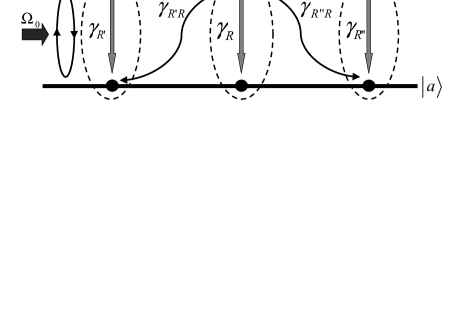
Figure 1: Scheme associated to the fluorophore evolution Eq. (II.5), see text.

The Lindblad rate equation Eq. (II.5) is the central result of this section. It effectively describes the action of the nanoscopic fluctuating environment over the fluorophore. The scheme of Figure 1 symbolically represents all processes associated to this equation. The first line of Eq. (II.5) describe the self-system dynamic for each configurational state $\left|R\right\rangle.$ The decay rate {$\gamma_{R}$}, the natural transition frequency {$\omega_{R}$}, as well as the Rabi frequency {$\Omega_{R}$} may depend on the bath state. The second line describe transitions between the configurational states (with rates {$\phi_{R^{\prime}R}$}), whose dynamic does not depend on the state of the fluorophore (property symbolically represented in Fig. 1 by the surrounding ellipse). Finally, the third line describes configurational transitions that are attempted by a transition between the upper and lower states of the system (rates {$\gamma_{R^{\prime}R}$}). In Sec. IV, a detailed analysis of each contribution and its associated “kinetic environment evolution” [i.e., the dynamics of $P_{R}(t),$ Eq. (18)] is presented.

As neither the initial conditions or the dynamics [Eq. (II.5)] introduce any coherence between the bath macrostates, their density matrix can be written as $\rho_{\mathcal{U}}(t)=\sum\nolimits_{R}P_{R}(t)\left|R\right\rangle\left\langle R\right|.$ From the relation $\mathrm{Tr}_{\mathcal{U}}[O_{\mathcal{U}}\rho_{\mathcal{U}}(t)]=\mathrm{Tr}_{\mathcal{U}}[O_{\mathcal{U}}(t)\rho_{\mathcal{U}}(0)],$ it follows that the dynamics of operators $O_{\mathcal{U}}(t)$ acting on $\mathcal{H}_{\mathcal{U}}$ is classical and dictated by the probabilities $P_{R}(t).$ On the other hand, the system dynamic arise after “tracing out” [Eq. (17)] all internal transitions between the configurational states of the reservoir (see Fig. 1). Therefore, the evolution of the system density matrix must be highly non-Markovian. In fact, taking into account the results presented in Ref. rate , it follows

$$\frac{d\rho_{\mathcal{S}}(t)}{dt}=\mathcal{L}_{H}\rho_{\mathcal{S}}(t)+\int_{0}^{t}d\tau\mathbb{L}(t-\tau)\rho_{\mathcal{S}}(\tau).$$ (28)

$\mathcal{L}_{H}$ defines the system unitary dynamic. The equation that defines the superoperator $\mathbb{L}$ can be explicitly written in a Laplace domain in terms of the propagator associated to Eq. (II.5) (see Eqs. (58) and (62) in Ref. rate ).

III Scattered field observables

In SMS experiments, the fluorophore dynamic is indirectly probed by subjecting the system to laser radiation [Eq. (25)] and measuring the scattered electromagnetic field. Therefore, while the master Eq. (II.5) completely characterizes the system dynamic, one is mainly interested in observables associated to the scattered laser field. In general, these observables can be written as a function of the electric field. For example, the flux of energy $S_{\mathcal{F}}$ per unit area per unit time (module of the Pointyng vector) reads landau

$$S_{\mathcal{F}}(t)=\frac{1}{2}\frac{c}{4\pi}|\mathbf{E}(t)\times\mathbf{H}(t)^{{\dagger}}|=\frac{c}{8\pi}\sqrt{\frac{\varepsilon}{\mu}}|\mathbf{E}(t)|^{2},$$ (29)

where the second equality follows from the relation between $\mathbf{E}(t)$ and $\mathbf{H}(t)$ [see Eq. (4)].

The time evolution of the electric field operator follows from a Heisenberg evolution with respect to the total Hamiltonian Eq. (16), i.e., $(d/dt)\mathbf{E}(t)=(i/\hbar)[H_{\mathcal{T}},\mathbf{E}(t)].$ Taking into account Eq. (4a), the time dependence of $\mathbf{E}(t)$ can be obtained from the evolution of the operators $a_{\mathbf{k}\lambda}^{(R)}\equiv a_{\mathbf{k}\lambda}^{(R)}\left|R\right\rangle\left\langle R\right|.$ We get

$$\frac{da_{\mathbf{k}\lambda}^{(R)}(t)}{dt}\simeq-i\omega_{\mathbf{k}}^{(R)}a_{\mathbf{k}\lambda}^{(R)}(t)-i\sum_{R^{\prime}}\kappa_{RR^{\prime}}^{\mathbf{k},\lambda^{\ast}}\sigma_{R^{\prime}R}(t),$$ (30)

where $\omega_{\mathbf{k}}^{(R)}$ and the coefficients $\kappa_{RR^{\prime}}^{\mathbf{k},\lambda}$ are defined by Eqs. (5) and (12) respectively. Furthermore, the $\mathcal{SU}$ operator $\sigma_{R^{\prime}R}$ is defined by

$$\sigma_{R^{\prime}R}\equiv\sigma\left|R^{\prime}\right\rangle\left\langle R\right|.$$ (31)

Eq. (30) relies on a set of approximations consistent with the effective representation of the reservoir. Since the dielectric constant of each configurational state is well defined, any non-diagonal non-linear coupling between the field modes is discarded. Terms arising from $H_{\mathcal{U}}^{\prime}$ [Eq. (13)] are also disregarded because they only introduce a small modification to the natural (optical) frequency of each mode.

The dynamics of $a_{\mathbf{k}\lambda}^{(R)}(t)$ can be written as the addition of two contributions, each one associated to the homogeneous and inhomogeneous terms in Eq. (30). Then, the electric field is written as carmichaelbook ; breuerbook

$$\mathbf{E}(t)=\mathbf{E}_{\mathrm{f}}(t)+\mathbf{E}_{\mathrm{s}}(t).$$ (32)

The contribution $\mathbf{E}_{\mathrm{f}}(t)$ defines the free evolution of the field. In terms of positive and negative frequency contributions, $\mathbf{E}_{\mathrm{f}}(t)=\mathbf{E}_{\mathrm{f}}^{(+)}(t)+\mathbf{E}_{\mathrm{f}}^{(-)}(t),$ it is defined by

$$\mathbf{E}_{\mathrm{f}}^{(+)}(t)=i\sum_{R,\mathbf{k},\lambda}\left|R\right\rangle\left\langle R\right|\sqrt{\frac{\hbar\omega_{\mathbf{k}}^{(R)}}{2V\varepsilon_{R}}}\hat{e}_{\mathbf{k}\lambda}e^{-i(t\omega_{\mathbf{k}}^{(R)}-\mathbf{k\cdot r})}a_{\mathbf{k}\lambda}(0).$$ (33)

The scattered field contribution $\mathbf{E}_{\mathrm{s}}(t)$, associated to the inhomogeneous term in Eq. (30), after some algebra carmichaelbook can be written as $\mathbf{E}_{\mathrm{s}}(t)=\mathbf{E}_{\mathrm{s}}^{(+)}(t)+\mathbf{E}_{\mathrm{s}}^{(-)}(t),$ where

$$\mathbf{E}_{\mathrm{s}}^{(+)}(t)=\frac{\omega_{A}^{2}}{4\pi c^{2}r}[(\mathbf{\hat{d}}\times\mathbf{\hat{r}})\times\mathbf{\hat{r}]}\sum_{RR^{\prime}}d_{RR^{\prime}}\sigma_{R^{\prime}R}(t-r/c_{R}),$$ (34)

with $\mathbf{\hat{r}\equiv r}/|\mathbf{r}|,$ $r\equiv|\mathbf{r}|,$ and $c_{R}=c/\sqrt{\varepsilon_{R}}.$ As before [Eq. (24)], for simplicity we assumed that $\mathbf{d}_{R^{\prime}R}=d_{R^{\prime}R}\mathbf{\hat{d}}.$

The previous expression allows to obtain the electric field in terms of operators defined in the system and configurational Hilbert spaces. Consistently with the effective representation of the reservoir, it is rewritten as

$$\mathbf{E}_{\mathrm{s}}^{(+)}(t)=\sum_{RR^{\prime}}\mathbf{E}_{\mathrm{s}(R|R^{\prime})}^{(+)(t)}[\left|R^{\prime}\right\rangle\left\langle R\right|](t),$$ (35)

where each contribution reads

$$\mathbf{E}_{\mathrm{s}(R|R^{\prime})}^{(+)(t)}=\frac{\omega_{A}^{2}}{4\pi c^{2}r}[(\mathbf{\hat{d}}\times\mathbf{\hat{r}})\times\mathbf{\hat{r}]}\ d_{RR^{\prime}}\sigma_{R^{\prime}}^{\mathrm{c}}(t-r/c_{R}).$$ (36)

Since the background electromagnetic field [Eq. (4a)] does not involve any coherence between the configurational states, the operator $[\left|R^{\prime}\right\rangle\left\langle R\right|](t)$ appearing in Eq. (35) must be read as follows. It labels all contributions to $\mathbf{E}_{\mathrm{s}}^{(+)}(t)$ that at time $t$ are attempted by the configurational transition $\left|R^{\prime}\right\rangle\rightarrow\left|R\right\rangle,$ ($R\neq R^{\prime}$). Then, the “conditional operator” $\mathbf{E}_{\mathrm{s}(R|R^{\prime})}^{(+)(t)}$ defines the electric field restricted to the condition that at time $t$ the reservoir is in the configurational state $\left|R^{\prime}\right\rangle$ and change to the state $\left|R\right\rangle.$ Similarly, the diagonal contributions $\mathbf{E}_{\mathrm{s}(R|R)}^{(+)(t)}$ define the electric field “given” that at time $t$ the reservoir is in the configurational state $\left|R\right\rangle.$ Consistently, the conditional operator $\sigma_{R}^{\mathrm{c}}(t)$ gives the evolution of the system operator $\sigma(t)$ under the same condition.

Any scattered field observable must be written in terms of the conditional system operators $\mathbf{E}_{\mathrm{s}(R|R^{\prime})}^{(+)(t)}.$ Below, we characterize the field correlations.

III.1 Correlations

When the scattered field is measured with photoelectric detectors, the usual observables can be written in terms of two time (normal order) correlations breuerbook ; carmichaelbook ; milburn ; scully ; loudon

$$C_{1}(\tau)\equiv\lim_{t\rightarrow\infty}:\overline{\mathbf{E}_{\mathrm{s}}^{(-)}(t)\mathbf{E}_{\mathrm{s}}^{(+)}(t+\tau)}:,$$ (37)

as well as

$$C_{2}(\tau)\equiv\lim_{t\rightarrow\infty}:\overline{\mathbf{E}_{\mathrm{s}}^{(-)}(t)\mathbf{E}_{\mathrm{s}}^{(-)}(t+\tau)\mathbf{E}_{\mathrm{s}}^{(+)}(t+\tau)\mathbf{E}_{\mathrm{s}}^{(+)}(t)}:.$$ (38)

The overbar denotes quantum average with respect to the total initial density matrix. The symbol $:(\cdots):$ takes into account the right interpretation of Eq. (34) and denotes a summation over all internal configurational paths defined through the conditional contributions $\mathbf{E}_{\mathrm{s}(R|R^{\prime})}^{(+)(t)},$ Eq. (36). Then, the correlations are explicitly written as

$$C_{1}(\tau)=\lim_{t\rightarrow\infty}\sum_{R_{1},R_{2}}\sum_{R_{3},R_{4}}\overline{\mathbf{\tilde{E}}_{\mathrm{s}(R_{2}|R_{1})}^{(-)(t)}\mathbf{\tilde{E}}_{\mathrm{s}(R_{4}|R_{3})}^{(+)(t+\tau)}},$$ (39)

and

$$C_{2}(\tau)=\lim_{t\rightarrow\infty}\!\!\sum_{\begin{subarray}{c}R_{1},R_{2}\\ R_{3},R_{4}\end{subarray}}\!\overline{\mathbf{\tilde{E}}_{\mathrm{s}(R_{2}|R_{1})}^{(-)(t)}\mathbf{\tilde{E}}_{\mathrm{s}(R_{4}|R_{3})}^{(-)(t+\tau)}\mathbf{\tilde{E}}_{\mathrm{s}(R_{4}|R_{3})}^{(+)(t+\tau)}\mathbf{\ \tilde{E}}_{\mathrm{s}(R_{2}|R_{1})}^{(+)(t)}},$$ (40)

where $\mathbf{\tilde{E}}_{\mathrm{s}(R|R^{\prime})}^{(\pm)(t)}\equiv\mathbf{\ E}_{\mathrm{s}(R|R^{\prime})}^{(\pm)(t)}\varepsilon_{R^{\prime}}^{1/4}.$ This definition guarantees that both correlations can be related to observables defined in terms of energy (photon) fluxes [see Eq. (29)]. It also takes into account that before the transition $\left|R^{\prime}\right\rangle\rightarrow\left|R\right\rangle,$ the dielectric constant of the bath is $\varepsilon_{R^{\prime}}.$

By using Eq. (36) and the rate expressions Eq. (24), the first order correlation can be written as

$$C_{1}(\tau)=f(\mathbf{\hat{r}})\frac{\hbar\omega_{A}}{4\pi cr^{2}}\sum_{R,R^{\prime}}(\tilde{\gamma}_{R}\tilde{\gamma}_{R^{\prime}})^{1/2}\lim_{t\rightarrow\infty}\overline{\sigma_{R}^{{\dagger}\mathrm{c}}(t)\sigma_{R^{\prime}}^{\mathrm{c}}(t+\tau)},$$ (41)

where for brevity we define $f(\mathbf{\hat{r}})\equiv[(\mathbf{\hat{d}}\times\mathbf{\hat{r}})\times\mathbf{\hat{r}}]^{2},$ and

$$\tilde{\gamma}_{R}\equiv\gamma_{R}+\sum_{R^{\prime}}\gamma_{R^{\prime}R}.$$ (42)

Eq. (41) can be considered as a natural generalization of the expression corresponding to the Markovian case Markov . Similarly, the correlation of the (conditional) raising and lowering operators can also be obtained from the system density matrix evolution [Eq. (II.5)] after invoking to a quantum regression theorem. For Lindblad rate equations it reads QRT

$$\overline{O_{1}(t)A(t+\tau)O_{2}(t)}\!=\!\sum_{RR^{\prime}}\mathrm{Tr}_{\mathcal{S}}\{A(e^{\tau\hat{\mathcal{L}}})_{RR^{\prime}}[O_{2}\rho_{R^{\prime}}(t)O_{1}]\},$$ (43)

where $O_{1},$ $O_{2}$ and $A$ are arbitrary system operators. Each contribution [indexed by $R,R^{\prime}],$ defines a conditional average of the involved operators: at time $t,$ the configurational bath state is $\left|R^{\prime}\right\rangle,$ while at time $(t+\tau),$ it is $\left|R\right\rangle.$ $\hat{\mathcal{L}}$ denotes the generator of the Lindblad rate equation,

$$\rho_{R}(t)=\sum_{R^{\prime}}(e^{t\hat{\mathcal{L}}})_{RR^{\prime}}\rho_{R^{\prime}}(0).$$ (44)

From Eqs. (43) and Eq. (41) it follows

$$C_{1}(\tau)=f(\mathbf{\hat{r}})\frac{\hbar\omega_{A}}{4\pi cr^{2}}\sum_{RR^{\prime}}\sqrt{\tilde{\gamma}_{R}\tilde{\gamma}_{R^{\prime}}}\mathrm{Tr}_{\mathcal{S}}\{\sigma(e^{\tau\hat{\mathcal{L}}})_{RR^{\prime}}[\rho_{R^{\prime}}^{\infty}\sigma^{\dagger}]\},$$ (45)

where $\rho_{R}^{\infty}\equiv\lim_{t\rightarrow\infty}\rho_{R}(t).$ By using the same calculations steps, the second order correlation reads

$$C_{2}(\tau)\! = \!\Big{[}f(\mathbf{\hat{r}})\frac{\hbar\omega_{A}}{4\pi cr^{2}}\Big{]}^{2}\!\sum_{RR^{\prime}}\!\tilde{\gamma}_{R}\mathrm{Tr}_{\mathcal{S}}\Big{\{}\sigma^{\dagger}\sigma(e^{\tau\hat{\mathcal{L}}})_{RR^{\prime}}$$

$$\times\Big{[}\gamma_{R^{\prime}}\sigma\rho_{R^{\prime}}^{\infty}\sigma^{{\dagger}}+\mathop{\textstyle\sum}_{R^{\prime\prime}}\gamma_{R^{\prime}R^{\prime\prime}}\sigma\rho_{R^{\prime\prime}}^{\infty}\sigma^{{\dagger}}\Big{]}\Big{\}}.$$

The expressions Eqs. (45) and (III.1) are the central results of this section. They allow to characterize observables such as the spectrum of the radiated field as well as the intensity-intensity correlation.

III.2 Spectrum

The spectral intensity radiation (in units of energy $\hbar\omega_{A}$) per unit of solid angle carmichaelbook ; breuerbook is defined by the dimensionless expression

$$S(\omega)=\frac{1}{2\pi}\int_{-\infty}^{+\infty}d\tau e^{i(\omega-\omega_{L})\tau}\Big{(}\frac{\hbar\omega_{A}}{4\pi cr^{2}}\Big{)}^{-1}C_{1}(\tau),$$ (47)

where $\omega_{L}$ is the frequency of the laser excitation, [Eq. (25)]. As usually $\lim_{\tau\rightarrow\infty}C_{1}(\tau)\neq 0,$ the spectrum can be split in a coherent and incoherent contributions

$$S(\omega)=f(\mathbf{\hat{r}})[S_{coh}(\omega)+(2\pi)^{-1}S_{inc}(\omega)].$$ (48)

$S_{coh}(\omega)$ consists in a Dirac delta term

$$S_{coh}(\omega)\equiv S_{coh}^{(0)}\delta(\omega_{L}),$$ (49)

that measures the scattered radiation emitted at the frequency of the laser excitation. From Eq. (45), it follows

$$S_{coh}^{(0)}=\sum_{RR^{\prime}}\sqrt{\tilde{\gamma}_{R}\tilde{\gamma}_{R^{\prime}}}\left\langle b\right|\rho_{R}^{\infty}\left|a\right\rangle\left\langle a\right|\rho_{R^{\prime}}^{\infty}\left|b\right\rangle.$$ (50)

The incoherent contribution can be written as

$$S_{inc}(\omega)=\Big{[}\tilde{C}_{1}(u)|_{-i(\omega-\omega_{L})}+\tilde{C}_{1}(u)|_{i(\omega-\omega_{L})}\Big{]},$$ (51)

where $\tilde{C}_{1}(u)=\int_{0}^{\infty}d\tau e^{-u\tau}\tilde{C}_{1}(\tau)$ is the Laplace transform of the function $\tilde{C}_{1}(\tau)\equiv[\hbar\omega_{A}f(\mathbf{\hat{r}})/4\pi cr^{2}]^{-1}C_{1}(\tau).$

In a Markovian limit, i.e., when the configurational space is unidimensional, from Eq. (51) it is possible to write the spectrum as an addition of three Lorentzian functions (Mollow triplet) whose widths and heights depend on the natural decay of the system and the Rabi frequency breuerbook ; carmichaelbook ; milburn ; scully . In the general non-Markovian case, the spectrum also has a strong dependence on the parameters that define the environment fluctuations (see next sections). In spite of these dissimilarities, in both cases the spectrum is mainly related to the dynamic behavior of the system coherences [see Eq. (50)].

III.3 Intensity-Intensity correlation

The normalized intensity-intensity correlation milburn reads

$$g_{2}(\tau)=\lim_{t\rightarrow\infty}\frac{:\overline{\mathbf{I}(t+\tau)\mathbf{I}(t)}:}{\overline{\mathbf{I}(t)}^{2}}=\frac{C_{2}(\tau)}{|C_{1}(0)|^{2}},$$ (52)

where $\mathbf{I}(t)=\mathbf{E}_{\mathrm{s}}^{(-)}(t)\mathbf{E}_{\mathrm{s}}^{(+)}(t)\mathbf{\ }$is the intensity operator. From Eqs. (45) and (III.1) it follows

$$g_{2}(\tau)=\frac{1}{(\mathrm{I}_{\mathrm{st}})^{2}}\sum_{RR^{\prime}}\tilde{\gamma}_{R}\left\langle b\right|(e^{\tau\hat{\mathcal{L}}})_{RR^{\prime}}[a_{R^{\prime}}^{\infty}]\left|b\right\rangle,$$ (53)

where

$$a_{R^{\prime}}^{\infty}=\Big{\{}\gamma_{R^{\prime}}\left\langle b\right|\!\rho_{R^{\prime}}^{\infty}\!\left|b\right\rangle+\sum_{R^{\prime\prime}}\gamma_{R^{\prime}R^{\prime\prime}}\left\langle b\right|\!\rho_{R^{\prime\prime}}^{\infty}\!\left|b\right\rangle\Big{\}}\!\left|a\right\rangle\!\left\langle a\right|,$$ (54)

and the normalization constant reads

$$\mathrm{I}_{\mathrm{st}}=\sum\limits_{R}\tilde{\gamma}_{R}\left\langle b\right|\rho_{R}^{\infty}\left|b\right\rangle.$$ (55)

As in the Markovian case carmichaelbook , Eq. (53) corresponds to the probability density of detecting one photon in the stationary regime ($\lim_{t\rightarrow\infty}$) and a second one in the interval $(\tau,\tau+d\tau).$ The factor $a_{R^{\prime}}^{\infty}$ takes into account all possible emission paths that leave the system in the ground state and the reservoir in the configurational state $\left|R^{\prime}\right\rangle.$ The sum over the index $R$ takes into account all photon emissions that happen in the interval $(\tau,\tau+d\tau)$ and leave the reservoir in the state $\left|R\right\rangle.$ The normalization factor $\mathrm{I}_{\mathrm{st}}$ defines the average stationary intensity emitted by the fluorophore.

IV Photon counting statistics: a generating function approach

In most of the SMS experiments the scattered laser radiation is measured with photon detectors. Then, the photon counting statistics is also an usual observable. As in standard fluorescent systems, the probability $P_{n}(t)$ of detecting $n$ photons up to time $t$ follows from a Mandel formula carmichaelbook ; breuerbook . Here, it is generalized as

$$P_{n}(t)=\frac{1}{n!}:\overline{\Big{[}\int_{0}^{t}dt^{\prime}\mathbf{\hat{I}}(t^{\prime})\Big{]}^{n}\exp\Big{[}-\int_{0}^{t}dt^{\prime}\mathbf{\hat{I}}(t^{\prime})\Big{]}}:,$$ (56)

where the normalized intensity operator $\mathbf{\hat{I}}(t)=(\hbar\omega_{A}/4\pi cr_{d}^{2})^{-1}\mathbf{E}_{\mathrm{s}}^{(-)}(t)\mathbf{E}_{\mathrm{s}}^{(+)}(t)$ has units of photon flux. $r_{d}$ denotes the distance between the fluorophore and the detector. $:(\cdots):$ denotes both an usual (normal) time ordering and a summation over all internal configurational paths, whose definition follows straightforwardly from Eqs. (39) and (40).

While Eq. (56) allows to characterize the probabilities $P_{n}(t),$ a simpler technique to calculate these objects is provided by a generating function approach cook ; mukamelPRA . This very well known technique was also used in the context of SMS when dealing with stochastic Bloch equations zheng ; FLHBrown ; he ; BarkaiExactMandel and related approximations. In contrast, here we formulate the generating function approach cook ; mukamelPRA on the basis of one of the central results of this contribution, i.e., Eq. (II.5). Added to its broad generality, the present formulation avoid the use of any stochastic calculus.

By writing the system density matrix as

$$\rho_{\mathcal{S}}(t)=\sum\nolimits_{n=0}^{\infty}\rho^{(n)}(t),$$ (57)

where each state $\rho^{(n)}(t)$ corresponds to the system state conditioned to $n-$photon detection events plenio ; carmichaelbook , the probability of counting $n$-photons up to time $t$ reads

$$P_{n}(t)=\mathrm{Tr}_{\mathcal{S}}[\rho^{(n)}(t)].$$ (58)

A “generating operator” cook is defined by

$$G(t,s)\equiv\sum\nolimits_{n=0}^{\infty}s^{n}\rho^{(n)}(t),$$ (59)

where $s$ is an extra real parameter. This operator also encodes the system dynamic, $\rho_{\mathcal{S}}(t)=G(t,s)|_{s=1}.$ The conditional states $\rho^{(n)}(t)$ can be decomposed into the contributions associated to each configurational state of the reservoir, leading to the expression

$$G(t,s)=\sum\nolimits_{n=0}^{\infty}s^{n}\sum\nolimits_{R}\rho_{R}^{(n)}(t)\equiv\sum\nolimits_{R}G_{R}(t,s).$$ (60)

Each matrix $\rho_{R}^{(n)}(t)$ defines the state of the system under the condition that, at time $t,$ $n-$photon detection events happened and the configurational state of the environment is $\left|R\right\rangle.$ Consistently, each contribution $G_{R}(t,s)$ defines the (conditional) generating operator “given” that the reservoir is in the configurational state $\left|R\right\rangle.$ Its evolution, from Eq. (II.5), can be written as

$$\dfrac{dG_{R}(t,s)}{dt}\! = \!\dfrac{-i}{\hbar}[H_{R},G_{R}(t,s)]-\tilde{\gamma}_{R}\{D,G_{R}(t,s)\}_{+}$$

$$\!+\sum\limits_{R^{\prime}}\phi_{RR^{\prime}}G_{R^{\prime}}(t,s)\!-\!\sum\limits_{R^{\prime}}\phi_{R^{\prime}R}G_{R}(t,s)$$

$$\!+s\gamma_{R}\mathcal{J}[G_{R}(t,s)]+s\sum\limits_{R^{\prime}}\gamma_{RR^{\prime}}\mathcal{J}[G_{R^{\prime}}(t,s)],$$

where $\tilde{\gamma}_{R}$ is defined by Eq. (42). Notice that the parameter $s$ is introduced in all terms (third line) associated to a photon detection event, i.e., those proportional to $\sigma\bullet\sigma^{\dagger}$ plenio ; carmichaelbook .

In the context of SMS zheng ; FLHBrown ; he ; BarkaiExactMandel , the matrix elements of $G(t,s),$ in an interaction representation with respect to $\hbar\omega_{L}\sigma_{z},$ are usually denoted as

$$\mathcal{U}(t,s) \equiv \frac{1}{2}(G_{ab}e^{-i\omega_{L}t}+G_{ba}e^{i\omega_{L}t}),$$ (62a)

$$\mathcal{V}(t,s) \equiv \frac{1}{2i}(G_{ab}e^{-i\omega_{L}t}-G_{ba}e^{i\omega_{L}t}),$$ (62b)

$$\mathcal{W}(t,s) \equiv \frac{1}{2}(G_{bb}-G_{aa}),$$ (62c)

$$\mathcal{Y}(t,s) \equiv \frac{1}{2}(G_{bb}+G_{aa}),$$ (62d)

[$$G_{pq}\equiv\left\langle p\right|G(t,s)\left|q\right\rangle], R.$$ while their evolution is called “generalized optical Bloch equation.” From Eq. (60), it is possible to write each matrix element as a sum over the parameter In Appendix A, we provide the evolution of each component [Eq. (88)].

After getting the matrix elements of the generating operator, Eq. (62), the photon counting process can be characterized in a standard way vanKampen . From the definition of the generating operator, Eq. (59), the photon counting probabilities Eq. (58) follows as

$$P_{n}(t)=\frac{2}{n!}\left.\frac{\partial^{n}}{\partial s^{n}}\mathcal{Y}(t,s)\right|_{s=0}.$$ (63)

The function $\mathcal{Y}(t,s)$ also allows to calculate all factorial moments

$$\bar{N}^{(k)}(t)\equiv\sum_{n=0}^{\infty}n(n-1)\cdots(n-k+1)P_{n}(t),$$ (64)

in terms of its derivatives

$$\bar{N}^{(k)}(t)=2\left.\frac{\partial^{k}}{\partial s^{k}}\mathcal{Y}(t,s)\right|_{s=1}.$$ (65)

Furthermore, the first two moments of the photon counting process, $\overline{N^{k}}(t)\equiv\sum_{n=0}^{\infty}n^{k}P_{n}(t),$ ($k=1,2$), read

$$\overline{N}(t) = 2\left.\frac{\partial}{\partial s}\mathcal{Y}(t,s)\right|_{s=1},$$ (66a)

$$\overline{N^{2}}(t) = 2\left.\frac{\partial^{2}}{\partial s^{2}}\mathcal{Y}(t,s)\right|_{s=1}+2\left.\frac{\partial}{\partial s}\mathcal{Y}(t,s)\right|_{s=1}.\ \ \ \$$ (66b)

Both moments encode important information about the scattered radiation. The line shape of the fluorophore system is defined by barkaiChem

$$\mathrm{I}(\omega_{L})\equiv\lim_{t\rightarrow\infty}\frac{d}{dt}\overline{N}(t),$$ (67)

while the Mandel factor is defined as

$$Q(t)\equiv\frac{\overline{N^{2}}(t)-\overline{N}^{2}(t)}{\overline{N}(t)}-1.$$ (68)

As is well known breuerbook ; carmichaelbook ; milburn ; scully , it allows to determining the sub- or super-Poissonian character of the photon counting process. In Appendix B we show the consistency between the generating function approach, the Mandel formula Eq. (56), and the results obtained in the previous section. In Appendix C, it is shown that the stationary Mandel factor

$$Q_{st}\equiv\lim_{t\rightarrow\infty}Q(t),$$ (69)

can be obtained in an exact analytical way after solving the evolution Eq. (IV) in the Laplace domain.

V Examples

In this section, different processes covered by Eq. (II.5) are analyzed. The examples are classified in accordance with the evolution of the environment fluctuations, i.e., the evolution of the configurational populations $P_{R}(t),$ Eq. (18). In each case, observables such as the spectrum Eq. (47), intensity-intensity correlation, Eq. (53), line shape, Eq. (67), and Mandel factor, Eq. (68), can be calculated in an exact analytical way. In fact, in a Laplace domain, both the evolution of the auxiliary density states, Eq. (II.5), and the evolution of the auxiliary generating operators, Eq. (IV), become algebraic linear equations.

V.1 Self environment fluctuations

When the nano-reservoir only has dense manifold of states, the fluctuations between the configurational states must be governed by a classical master equation vanKampen . This case is covered by taking

$$\dfrac{d\rho_{R}(t)}{dt} = \frac{-i}{\hbar}[H_{R},\rho_{R}(t)]-\gamma_{R}(\{D,\rho_{R}(t)\}_{+}-\mathcal{J}[\rho_{R}(t)])$$ (70)

$$-\sum\limits_{R^{\prime}}\phi_{R^{\prime}R}\rho_{R}(t)+\sum\limits_{R^{\prime}}\phi_{RR^{\prime}}\rho_{R^{\prime}}(t),$$

which arises from Eq. (II.5) under the condition $\mathbf{d}_{RR^{\prime}}=0,$ $R\neq R^{\prime},$ implying the vanishing of the rates $\{\gamma_{RR^{\prime}}\}$ [Eq. (24)]. From Eq. (70), the evolution of the configurational populations, Eq. (18), reads

$$\frac{d}{dt}P_{R}(t)=-\sum\limits_{R^{\prime}}\phi_{R^{\prime}R}P_{R}(t)+\sum\limits_{R^{\prime}}\phi_{RR^{\prime}}P_{R^{\prime}}(t).$$ (71)

In the context of SMS, this evolution defines the “kinetic dynamic” of the environment. Consistently, this equation, and in consequence the transitions between the configurational states $\{\left|R\right\rangle\}_{R=1}^{R_{\max}}$, does not depend on the state of the system. Notice that in the effective microscopic representation, the configurational transitions are induced by the reservoir $\mathcal{W},$ Eq. (13).

While the fluctuations between the configurational states are defined by the classical evolution Eq. (71), the quantum dynamic of the system, for each bath state, is defined by the diagonal contribution in Eq. (70). Depending on its properties, different processes are recovered.

V.1.1 Spectral fluctuations

A nano-environment consisting on molecules at very low temperatures may induce random fluctuations in the natural frequency of a fluorophore barkaiChem . This situation can be described by the present formalism by assuming that the natural frequency of the system, Eq. (20), is the unique parameter that depends on the configurational bath states. Consequently, each configurational bath state has associated a different system transition frequency, $\omega_{R}=\omega_{A}+\delta\omega_{R}.$ Equivalently, each configurational state “induces” a spectral shift defined by the parameter $\delta\omega_{R}.$ The population $P_{R}(t)$ gives the probability that, at time $t,$ the natural frequency of the system is $\omega_{R}.$ The coefficients associated to the Rabi frequency, Eq. (27), must be chosen all the same. Similarly, the decay rates associated to each bath state, Eq. (24), are also all the same. Therefore, the system is characterized by one single Rabi frequency and a natural decay rate, i.e.,

$$\Omega_{R}=\Omega,\ \ \ \ \ \ \ \ \ \ \ \ \ \ \ \gamma_{R}=\gamma.$$ (72)

In the following analysis, the configurational space is assumed two dimensional, $R=1,2.$ Furthermore, the problem is restricted to a symmetrical one. The characteristic parameters read

$$\delta\omega_{A}^{(1)} = +\delta\omega,\ \ \ \ \ \ \ \ \ \ \ \ \ \ \ \ \ \ \phi_{21}=\phi,$$ (73a)

$$\delta\omega_{A}^{(2)} = -\delta\omega,\ \ \ \ \ \ \ \ \ \ \ \ \ \ \ \ \ \ \phi_{12}=\phi.$$ (73b)

With these assumptions, from the results of Appendix C, it is possible to characterize both the line shape, Eq. (67), and the stationary Mandel factor, Eq. (69), in an exact analytical way. The final expressions recover the results obtained by He and Barkai in Ref. BarkaiExactMandel , where the natural frequency of the fluorophore is modeled through a stochastic two-state process.

Figure 2: Optical spectra [Eq. (51)] for a fluorophore system subject to spectral fluctuations in the regime $\phi\ll\delta\omega\ll\gamma\simeq\Omega.$ (a) The parameters, in units of the decay rate $\gamma,$ are $\Omega=\gamma/\sqrt{2},$ $\delta\omega=\gamma/10,$ and $\phi=\gamma/125.$ (b) The parameters are $\Omega=5\gamma,$ $\delta\omega=\gamma/10,$ and $\phi=\gamma/500.$ The inset shows the narrow spectral peak. In both cases, the laser frequency is in resonance with the system, $\omega_{L}=\omega_{A}.$

Now, going beyond the possibilities of any previous approach, in the following figures we characterize the spectrum of the scattered radiation [Eq. (51)]. Its exact analytical expression is not provided due to its extension. In all cases, the system-laser detuning [Eq. (26)] is zero, i.e., $\omega_{L}=\omega_{A}.$ When the characteristic time between configurational transitions, $\phi^{-1},$ is the small time scale of the problem, the spectrum shape strongly depends on the relation between the natural decay $\gamma,$ the Rabi frequency $\Omega,$ and the spectral shift $\delta\omega.$ In Fig. 2, the condition $\phi\ll\delta\omega\ll\gamma\simeq\Omega$ is satisfied. Then, the spectral fluctuations induced by the bath slightly modify quantum dynamic of the system. Nevertheless, the spectrum shape presents strong deviations with respect to the Markovian case.

In Fig. 2a, as $\Omega<\gamma,$ the spectrum only consists in one Lorentzian component (Rayleigh peak) plenio . In contrast to standard (Markovian) fluorescent systems, here a central narrow peak is clearly visible. It must not be confused with the coherent Dirac delta contribution that appears in both Markovian and non-Markovian systems [Eq. (49)]. In fact, as in three level systems plenio , its origin can be related to the dynamics of the system coherences despuez . The spectrum develops a narrow peak whenever the dynamic of the coherences slowly fluctuates between two different regimes. The width of the narrow peak is given by the addition of the constant rates that define the fluctuations between the different dynamical regimes plenio . Here, as $\phi\ll\delta\omega,$ each dynamical regime is defined by the spectral shifts $\pm\delta\omega$ associated to each configurational bath state. The “blinking” between these two regimes is governed by the rate $\phi.$ Therefore, the width of the narrow peak is $2\phi,$ which allows us to read a central property of the environment fluctuations from the optical spectra.

Figure 3: Optical spectra [Eq. (51)] for a fluorophore system subject to spectral fluctuations in the regimes $\phi\ll\gamma\simeq\Omega\ll\delta\omega$ (a) and $\phi\ll\gamma\ll\Omega\simeq\delta\omega$ (b). In (a) the parameters, in units of the decay rate $\gamma,$ are $\Omega=\gamma/\sqrt{2},$ $\delta\omega=5\gamma,$ and $\phi=\gamma/(4\times 10^{4}).$ In (b) the parameters are $\Omega=5\gamma,$ $\delta\omega=5\gamma,$ and $\phi=\gamma/(4\times 10^{4}).$ In both cases, the laser frequency is in resonance with the system, $\omega_{L}=\omega_{A}.$ The insets corresponds to the central narrow peaks.

In Markovian fluorescent systems, when $\Omega>\gamma$ the laser strongly couples the population and coherences of the system, leading to oscillations that induce two extra peaks in the optical spectra (Mollow triplet) carmichaelbook . Here, this phenomenon is shown in Fig. 2b, where the parameters satisfy $\phi\ll\delta\omega\ll\gamma<\Omega.$ As the Rabi frequency $\Omega$ is much larger than the spectral shifts $\delta\omega,$ the peaks appear at $\pm\Omega.$ Consistently with the parameter values, the extra narrow peak (inset) is also associated with the coherences blinking-like evolution.

In Fig. 3a, the condition $\phi\ll\gamma\simeq\Omega\ll\delta\omega$ is satisfied. Therefore, the quantum system dynamic is mainly governed by the spectral shifts induced by the environment. Consistently, the spectrum develops two peaks at $\pm$ $\delta\omega.$ In contrast with the Mollow triplet, which is associated to the Rabi oscillations, here the central Rayleigh peak ($\omega_{L}=\omega_{A}$) is almost absent. It only appears a narrow central peak (inset) related to the coherence dynamics.

By maintaining the value of all parameters, in Fig. 3b, the laser intensity was increased such that $\phi\ll\gamma\ll\Omega\simeq\delta\omega.$ In this situation, there is a competition between the Rabi oscillations and the spectral shifts induced by the laser and the reservoir respectively. Notice that the extra peaks do not appear at $\pm\Omega$ [Fig. 2b] neither at $\pm\delta\omega$ [Fig. 3a]. Furthermore, in contrast to standard fluorescent systems, the height of the central Rayleigh peak is smaller than the height of the lateral peaks. The inset shows the narrow central peak. Since the parameters of the environmental fluctuations are the same than in Fig. 3a, the central narrow peaks have the same widths, i.e., $2\phi.$

Figure 4: Optical spectra [Eq. (51)] for a fluorophore system subject to spectral fluctuations. In (a) the parameters, in units of the decay rate $\gamma,$ are $\Omega=\gamma/\sqrt{2},$ $\delta\omega=5\gamma,$ and $\phi=10\gamma$ (dashed line), $\phi=50\gamma$ (dotted line), $\phi=125\gamma$ (solid line). In (b) the parameters are $\Omega=\gamma,$ $\delta\omega=3\gamma,$ and $\phi=0.25\gamma$ (dashed line), $\phi=\gamma$ (dotted line), $\phi=4\gamma$ (solid line). In both cases, the laser frequency is in resonance with the system, $\omega_{L}=\omega_{A}.$

A broad kind of spectrum behavior may arise when the environment fluctuation time $\phi^{-1}$ is not the small time scale of the problem. In this regime, the coherences dynamic loose its dichotomic character and consequently the spectrum does not develop any central narrow peak despuez . In Fig. 4a the reservoir fluctuations are faster than the system dynamic, $\gamma\simeq\Omega\simeq\delta\omega\ll\phi.$ The spectrum develops the well-known effect of motional narrowing, i.e., by increasing the rate $\phi$ the optical spectrum becomes narrow. In Fig. 4b the rate $\phi$ is increased around the intermediate regime $\gamma\simeq\phi.$ As the parameters of the system and the environment fluctuations are of the same order, a small variation of $\phi$ lead to strong changes in the spectral shape. This property can also be found in the photon counting statistics (see Fig. 5 in Ref. BarkaiExactMandel ).

V.1.2 Lifetime fluctuations

Chemical or physical conformational changes of the supporting nano-environment may modify the lifetime of the fluorophore barkaiChem ; michel ; jung . This situation is covered by taking $(\gamma_{RR^{\prime}}=0)$

$$\Omega_{R}=\Omega,\ \ \ \ \ \ \ \ \ \ \ \ \ \ \ \delta\omega_{R}=0.$$ (74)

Then, each configurational state $\left|R\right\rangle$ has associated the natural decay $\gamma_{R}.$ The classical evolution Eq. (71) describe the transitions, with rates $\phi_{R^{\prime}R},$ between the different decay rates felt by the fluorophore.

V.1.3 Molecules diffusing in solution

The present formalism may also be applied for describing the statistical properties of radiation patterns produced by molecules diffusing in a solution michel ; Elson . If the intensity of the laser field varies appreciably along the diffusing space, the Rabi frequency (which depends linearly on the external laser power) must be considered dependent on position. Then, the configurational space can be associated to the physical space where the diffusion process happens. This situation is covered by taking $(\gamma_{RR^{\prime}}=0)$

$$\gamma_{R}=\gamma,\ \ \ \ \ \ \ \ \ \ \ \ \ \ \ \ \delta\omega_{R}=0.$$ (75)

Each coefficient $\Omega_{R}$ [Eq. (27)] measures the laser intensity at each position labeled by the index $R.$ The evolution Eq. (71) describes the molecule diffusion. For an homogeneous coupling between first neighbors, $\phi_{RR\pm 1}=\phi,$ a standard diffusion process with diffusion coefficient $D_{0}=\Delta x^{2}\phi,$ is recovered. $\Delta x$ is the discretization step in physical space.

V.2 Light assisted environment fluctuations

When the local nano-reservoir surrounding the system only consists in a few degrees of freedom, its Hilbert space is defined by a discrete (finite) set of states. Therefore, each one may represents a different configurational state. While there exist different Lindblad rate equations that may model this situation (see end of this section), here we consider the case

$$\dfrac{d\rho_{R}(t)}{dt}\!\! = \!\!\dfrac{-i}{\hbar}[H_{R},\rho_{R}(t)]\!-\!\gamma_{R}(\{D,\rho_{R}(t)\}\!_{+}-\!\mathcal{J}[\rho_{R}(t)])$$ (76)

$$\!\!\!\!\!-\!\sum\limits_{R^{\prime}}\!\gamma_{R^{\prime}\!R}\{\!D,\rho_{R}(t)\}\!_{+}+\!\sum\limits_{R^{\prime}}\!\gamma_{RR^{\prime}}\mathcal{\ J}\![\rho_{R^{\prime}}(t)].$$

This evolution follows from Eq. (II.5) after taking $\{\phi_{RR^{\prime}}\}=0,$ condition consistent with the finite structure of the reservoir, i.e., its dynamic is unable to induces self (internal) fluctuations vanKampen . In the effective microscopic representation, it follows from the interaction Eq. (16) by uncoupling the configurational space from the reservoir $\mathcal{W},$ i.e., $H_{\mathcal{UW}}=0$ [Eq. (15)].

Taking into account the interaction Hamiltonian Eq. (11), we deduce that transitions between the different configurational bath states may only happen when they are attempted by a photon emission process, i.e., a transition between the upper and lower system states (see Fig. 1). Therefore, in contrast with the previous case, here the dynamic of the configurational populations [Eq. (18)] strongly depends on the state of the system. From Eq. (76) we get

$$\frac{d}{dt}P_{R}(t)=-\sum\limits_{R^{\prime}}\gamma_{R^{\prime}R}P_{R}^{(b)}(t)+\sum\limits_{R^{\prime}}\gamma_{RR^{\prime}}P_{R^{\prime}}^{(b)}(t),$$ (77)

where $P_{R}^{(b)}(t)\equiv\left\langle b\right|\rho_{R}(t)\left|b\right\rangle.$ The evolution of $P_{R}^{(b)}(t)$ also follows from Eq. (76), which in turn involves the remaining matrix elements of all auxiliary states. Therefore, in general it is not possible to write a simple equation for the evolution of the configurational populations. Nevertheless, in the limits $\{\gamma_{RR^{\prime}}\}\ll\{\gamma_{R}\}$ and $\{\gamma_{RR^{\prime}}\}\gg\{\gamma_{R}\},$ an evolution similar to Eq. (71) can be obtained. We assume that

$$\Omega_{R}=\Omega,\ \ \ \ \ \ \ \ \ \ \ \ \ \ \ \delta\omega_{R}=0,$$ (78)

implying that the fluorophore, independently of the configurational state, always feels the same laser intensity $\Omega,$ and maintains its transition frequency $\omega_{A}.$ These conditions allow to model a class of light assisted processes consistent with different experimental situations luzAssisted .

Under the condition $\{\gamma_{RR^{\prime}}\}\ll\{\gamma_{R}\},$ from Eq. (76) it is simple to realize that before happening a configurational transition, the fluorophore may emit a large number of photons. Thus, “while” the bath remains in the configurational state $\left|R\right\rangle,$ the fluorophore can be well approximated by a Markovian fluorescent system with decay rate $\tilde{\gamma}_{R}$ [Eq. (42)], the radiation pattern being characterized by the average intensity

$$I_{R}=\frac{\tilde{\gamma}_{R}\Omega^{2}}{\tilde{\gamma}_{R}^{2}+2\Omega^{2}+4\delta^{2}},$$ (79)

where $\delta=\omega_{L}-\omega_{A}$ is the system-laser detuning, Eq. (26). Consequently, it is possible to approximate

$$\tilde{\gamma}_{R}P_{R}^{(b)}(t)\simeq I_{R}P_{R}(t).$$ (80)

The first term represents the photon flux produced by the system while the bath remains in the configurational state $\left|R\right\rangle.$ This quantity is approximated by the intensity $I_{R}$ multiplied by the probability of being in the configurational state $\left|R\right\rangle,$ i.e., $P_{R}(t).$ Similarly, a straightforward interpretation of this approximation follows by noticing that $I_{R}/\tilde{\gamma}_{R}$ gives the stationary upper population of a Markovian optical transition with characteristic decay rate $\tilde{\gamma}_{R}.$ Then, Eq. (80) implies that, “given” that the reservoir remains in the state $\left|R\right\rangle,$ the upper population $P_{R}^{(b)}(t)$ quickly reaches the stationary value $I_{R}/\tilde{\gamma}_{R}.$

By introducing Eq. (80) in the evolution Eq. (77), it follows the classical evolution

$$\frac{d}{dt}P_{R}(t)\simeq-\sum\limits_{R^{\prime}}\Gamma_{R^{\prime}R}P_{R}(t)+\sum\limits_{R^{\prime}}\Gamma_{RR^{\prime}}P_{R^{\prime}}(t),$$ (81)

where the transition rates read

$$\Gamma_{R^{\prime}R}=\gamma_{R^{\prime}R}\left(\frac{\Omega^{2}}{\tilde{\gamma}_{R}^{2}+2\Omega^{2}+4\delta^{2}}\right).$$ (82)

These expressions generalize the results presented in Ref. luzAssisted . The associated radiation pattern develops a blinking phenomenon, i.e., the intensity of the scattered radiation randomly changes between the set of values $\{I_{R}\}$ associated to each configurational state. These changes are governed by the classical evolution Eq. (81). The dependence of the transition rates $\Gamma_{R^{\prime}R}$ on both the laser intensity and the system-laser detuning [compare with Eq. (71)], gives the light assisted character of the blinking phenomenon. In contrast with triplet blinking models barkaiChem ; molski , here all rates that govern the transitions between the configurational states (intensity states) depend on both, the laser intensity and the system laser detuning, the first property being consistent with different experimental results luzAssisted .

When $\{\gamma_{RR^{\prime}}\}\gg\{\gamma_{R}\},$ in the intermediate time between two consecutive configurational transitions, the system is only able to emits a few number of photons. Therefore, the blinking phenomenon is lost because it is not possible to associate an intensity regime [with value Eq. (79)] to each configurational state. In spite of this fact, under the replacement $\tilde{\gamma}_{R}\rightarrow(\sum_{R^{\prime\prime}}\gamma_{R^{\prime\prime}R})$ the approximation Eq. (80) is still valid. Since $\{\gamma_{RR^{\prime}}\}\gg\{\gamma_{R}\},$ it follows $\tilde{\gamma}_{R}\simeq(\sum_{R^{\prime\prime}}\gamma_{R^{\prime\prime}R}),$ implying that both Eq. (81) and (82) remain valid when $\{\gamma_{RR^{\prime}}\}\gg\{\gamma_{R}\}.$

Figure 5: Optical spectra [Eq. (51)] (a) and intensity-intensity correlation [Eq. (53)] (b) for a light assisted blinking radiation pattern. The configurational space is two dimensional, $R=1,2$. The parameter values, in units of the Rabi frequency $\Omega,$ are $\gamma_{1}=\Omega,$ $\gamma_{2}=10\Omega,$ $\gamma_{21}=0.0015\Omega,$ $\gamma_{12}=0.02\Omega.$ The laser is in resonance with the system, $\omega_{L}=\omega_{A}.$ In (a) the inset shows the central narrow peak.

In the following figures, the light assisted blinking phenomena described in Ref. luzAssisted is characterized through the scattered field observables. A two dimensional configurational space is assumed ($R=1,2$) and also the condition $\{\gamma_{RR^{\prime}}\}\ll\{\gamma_{R}\}$ is satisfied. Fig. 5a shows the optical spectrum [Eq. (51)]. The Rayleigh central peak is endowed with a narrow peak (inset). As in the previous analysis, it origin relies on the blinking like behavior of the system coherences, effect associated to Eq. (81). The width of the narrow peak despuez , $\Gamma_{12}+\Gamma_{21},$ depends on both the system-laser detuning and the laser intensity [see Eq. (82)].

Fig. 5b shows the normalized intensity-intensity correlation [Eq. (53)]. For short times, this function satisfies $0\leq g_{2}(\tau)<1,$ property associated to photon antibunching. At intermediates times the correlation satisfies $g_{2}(\tau)>1,$ indicating photon bunching, which in turn is a direct manifestation of the environment fluctuations. Furthermore, $g_{2}(\tau)$ is almost constant during a long period of time. This property is related with the telegraphic nature (high and low intensity states) of the scattered radiation field michel ; plenio .

The central narrow peak in the spectra as well as the photon bunching-antibunching transition reflected by the intensity-intensity correlation (Fig. 5) are associated to the blinking property of the scattered field intensity. Then, it is expected that, independently of the underlying dynamic, these features also arise whenever the radiated field fluctuates between two different intensity regimes. For example, the blinking phenomenon defined by Eq. (81) and (82), also can arises from a fluorophore whose environment, independently of the system state [Eq. (71)], randomly changes its natural decay between two different values, i.e., Eq. (70) with the parameters values Eq. (74). Consistently, we have checked that under the mapping

$$\gamma_{1} \rightarrow \tilde{\gamma}_{1}=(\gamma_{1}+\gamma_{21}),\ \ \ \ \ \ \ \ \ \ \phi_{21}=\Gamma_{21},$$ (83a)

$$\gamma_{2} \rightarrow \tilde{\gamma}_{2}=(\gamma_{2}+\gamma_{12}),\ \ \ \ \ \ \ \ \ \ \phi_{12}=\Gamma_{12},$$ (83b)

the spectrum [Eq. (51)] as well as the intensity correlation [Eq. (53)] associated to Eq. (70) [and Eq. (74)] are indistinguishable from those shown in Fig. 5. In spite of these similarities, both cases lead to very different photon counting processes.

Figure 6: Stationary Mandel factor [Eq. (69)] as a function of the system-laser detuning. For the light assisted process (full line) the parameters are the same than in Fig. 5. The inset shows the associated line shape [Eq. (67)]. For the self fluctuating environment (dotted line) the parameters are defined from the mapping Eq. (83). The dashed line corresponds to the scaling Eq. (85) with $\delta_{0}=\Omega,$ $\bar{\Omega}=0.25\Omega,$ and $\bar{\gamma}_{12}=0.007\Omega.$

In Fig. 6, the photon counting statistics is characterized through the stationary Mandel factor $Q_{st}$ [see Appendix C] as a function of the system-laser detuning, i.e., $\delta=\omega_{L}-\omega_{A}$ [Eq. (26)]. While the number of emitted photons (the stationary intensity) is inversely proportional to $\delta,$ in the limit of large detuning the Mandel factor may take arbitrary values. In fact, this object [Eq. (68)] measures the (normalized) fluctuations in the number of counted photons around its mean value. For the light assisted dynamic [Eq. (76)] (solid line), the photon statistic becomes super-Poissonian, i.e., $Q_{st}>0,$ with the asymptotic value

$$\lim_{\delta\rightarrow\infty}Q_{st}=\frac{2\gamma_{12}\gamma_{21}[(\gamma_{1}+\gamma_{21})-(\gamma_{2}+\gamma_{12})]^{2}}{(\gamma_{12}+\gamma_{21})^{2}(\gamma_{1}\gamma_{12}+\gamma_{2}\gamma_{21}+2\gamma_{12}\gamma_{21})}>0.$$ (84)

Notice that this expression does not depend on the external laser excitation. This result is expected because the condition $\Omega\ll\delta$ is satisfied. Instead, the photon counting statistic for the self fluctuating environment [Eq. (70)] (dotted line) becomes Poissonian for larger detuning, $\lim_{\delta\rightarrow\infty}Q_{st}=0.$ On the other hand, both dynamics are characterized by the same Mandel factor when the system-laser detuning is small. The inset shows the line shape Eq. (67) associated to the light assisted process.

The super-Poissonian character [$Q_{st}>0$] of the photon counting process in the limit of increasing system-laser detuning has a clear origin. For the light assisted process, all transition rates $\Gamma_{R^{\prime}R}$ [Eq. (82)] vanishes in the limit $\delta\rightarrow\infty.$ Instead, for the self-fluctuating environment the transition rates does not vanish in the same limit. In fact, they are independent of the properties of the external laser excitation, Eq. (71). The vanishing of $\lim_{\delta\rightarrow\infty}Q_{st}$ can be recover when the asymptotic value of one of the transition rates [Eq. (82)] does not depend on the system-laser detuning. This property can be achieved by assuming the following scaling (dashed line in Fig. 6)

$$\gamma_{12}\rightarrow\gamma_{12}+\bar{\gamma}_{12}(|\delta|/\delta_{0}),\ \ \ \ \ \ \ \ \ \ \ \ \ \ \ \Omega\rightarrow\Omega+\bar{\Omega}(|\delta|/\delta_{0})^{1/2},$$ (85)

where $\delta_{0},$ $\bar{\Omega},$ and $\bar{\gamma}_{12}$ are arbitrary constants. Both $\gamma_{12}$ and $\Omega$ increase as $\delta$ increases. Consequently, the transition rate $\Gamma_{12}$ does not vanish by increasing $\delta.$ In fact, $\lim_{\delta\rightarrow\infty}\Gamma_{12}\simeq\bar{\gamma}_{12}\bar{\Omega}^{2}/(\bar{\gamma}_{12}+4\delta_{0}^{2}).$ Furthermore, as $\gamma_{2}\ll\gamma_{12},$ “given” that the bath is in the configurational state $\left|2\right\rangle,$ most of the photon emissions are attempted by the transition $\left|2\right\rangle\rightarrow\left|1\right\rangle,$ implying $I_{2}\simeq 0.$ Therefore, with the scaling Eq. (85), the dynamic can be mapped with a triplet blinking modelling barkaiChem ; molski ; mandel where the configurational state $\left|2\right\rangle$ defines a dark state incoherently coupled to the system. On the other hand, by assuming valid the condition $\gamma_{21}\ll\gamma_{1},$ from Eqs. (79) and (82) it follows $I_{1}\simeq\gamma_{1}\bar{\Omega}^{2}/(4\delta_{0}|\delta|),$ and $\Gamma_{21}\simeq\gamma_{21}\bar{\Omega}^{2}/(4\delta_{0}|\delta|),$ which in turn implies that the bath state $\left|1\right\rangle$ can be associated to the bright intensity states. Finally, from Eq. (84), the scaling Eq. (85) implies $\lim_{\delta\rightarrow\infty}Q_{st}\simeq 2\gamma_{21}/\gamma_{1}\ll 1.$

V.3 General environment fluctuations

Having understood the derivation of Eq. (II.5) and their associated physical processes, one can quickly write down master equations that introduce more general environment fluctuations. The evolution of the auxiliary states is written as

$$\dfrac{d\rho_{R}(t)}{dt}=(\mathcal{L}_{H}^{(R)}+\mathcal{L}_{diag}^{(R)}+\mathcal{L}_{cf}^{(R)})[\rho_{R}(t)].$$ (86)

The superoperators $\mathcal{L}_{H}^{(R)}$ and $\mathcal{L}_{diag}^{(R)}$ define the unitary and irreversible evolution for each configurational bath state respectively. Both kind of contributions have been analyzed in the previous examples. Nevertheless, notice that extra pure dispersive contributions (phase destroying process) may also be considered. The non diagonal superoperator $\mathcal{L}_{cf}^{(R)}$introduces the more general environment fluctuations. It can be written as

$$\mathcal{L}_{cf}^{(R)}[\rho_{R}]=-\!\sum\limits_{\begin{subarray}{c}R^{\prime}\\ R^{\prime}\neq R\end{subarray}}\frac{\eta_{R^{\prime}R}}{2}\{A^{\dagger}A,\rho_{R}\}_{+}\!+\!\sum\limits_{\begin{subarray}{c}R^{\prime}\\ R^{\prime}\neq R\end{subarray}}\eta_{RR^{\prime}}A\rho_{R^{\prime}}A^{\dagger},$$ (87)

where the matrix $\eta_{R^{\prime}R}$ defines the characteristic non-diagonal rates of the problem. $A$ is an arbitrary system operator.

Only when $A=\mathrm{I},$ where the $\mathrm{I}$ is the identity operator, the environment fluctuations, defined by the evolution of $P_{R}(t),$ do not depend on the state of the system, recovering Eq. (70). When $A=\sigma=\left|a\right\rangle\left\langle b\right|,$ the evolution Eq. (76) is recovered, which is associated to bath fluctuations that are attempted by the system transition $\left|b\right\rangle\rightarrow\left|a\right\rangle,$ i.e., by a photon emission. When $A=\sigma^{\dagger}=\left|b\right\rangle\left\langle a\right|,$ the configurational transitions are attempted by a system transition from the lower to the upper state, $\left|a\right\rangle\rightarrow\left|b\right\rangle,$ i.e., the system absorbs a photon from the background electromagnetic field. This kind of contributions, which also arises from the microscopic interaction Eq. (11), were discarded because at room temperatures the optical thermal excitations are almost null.

For $A=\left|b\right\rangle\left\langle b\right|,$ Eq. (87) describes configurational transitions that can only happen when the fluorophore is in the upper state. These processes can be microscopically described by replacing the interaction Hamiltonian $H_{\mathcal{UW}},$ Eq. (15), by $\left|b\right\rangle\left\langle b\right|\otimes H_{\mathcal{UW}}.$ They induce light assisted processes similar to those described by Eq. (76). In particular, when $\delta\rightarrow\infty,$ the stationary photon counting statistics is also super-Poissonian. Similarly, $A=\left|a\right\rangle\left\langle a\right|,$ describes configurational transitions that only happen when the system is in the ground state. In both cases, the dynamic induced by Eq. (87) introduces a dephasing mechanism that affects the fluorophore yield.

The formalism does not forbid the situation in which $\eta_{R^{\prime}R}=0.$ This case was (partially) addressed in Refs. rapid ; mandel , where the underlying dynamic was defined in terms of a structured reservoir whose influence can be approximated by a direct sum of Markovian sub-reservoirs (generalized Born-Markov approximation) rate ; breuer . Most of the expressions for the scattered field observables obtained previously remain valid. Nevertheless, some properties of the radiation pattern may depend on which way the system-reservoir fluctuations are measured despuez .

VI Summary and Conclusions

The main theoretical problem of SMS is to relate the radiation of a single fluorophore system with the underlying dynamical fluctuations of its local environment. In this paper, we tackled this problem from a quantum-electrodynamic treatment based on an open quantum system approach.

The central ingredient of our formalism is the description of the nano-environment. Instead of considering the microscopic dynamics associated to each specific situation, after noting that the Hilbert space structure of the reservoir can not be resolved beyond the experimental resolution, it was approximated by a set of configurational macrostates, each one taking in account all microscopic bath configurations that lead to the same system dynamic. This coarse grained representation allows to define an effective microscopic description, where the fluorophore and background electromagnetic field Hamiltonians, as well as their mutual interaction, are parametrized by the configurational states. From the effective microscopic Hamiltonian, it was possible to achieve the central goals of this paper.

By tracing out the electromagnetic field and the configurational degrees of freedom, we derived the Lindblad rate evolution Eq. (II.5), which encode the statistical behavior of the fluorophore and the reservoir fluctuations.

In contrast with previous approaches, the scattered electromagnetic field was characterized from a full quantum-electrodynamic description. The electric field operator was written in terms of conditional system operators, Eq. (36). After appealing to a quantum regression theorem, they allow to expressing the field correlations in terms of the system density matrix propagator, Eqs. (45) and (III.1). High order correlations can also be expressed in a similar way. These results allow to get simple manageable expressions for observables like the spectrum, Eq. (48), and the intensity-intensity correlation, Eq. (53).

An extended Mandel formula, Eq. (56), which includes an additional sum over all configurational transitions, describe the photon counting statistics. A simpler characterization based on the generating operator Eq. (60) was presented. The line shape and stationary Mandel factor can be obtained straightforwardly after solving its evolution, Eq. (IV), in the Laplace domain.

The examples worked out in the manuscript were classified according to the properties of the configurational fluctuations. Processes like spectral diffusion and lifetime fluctuations correspond to bath fluctuations that do not depend on the system state while light assisted processes are recovered in the opposite case, i.e., when the environmental fluctuations become entangled with the system dynamic. From a microscopic point of view, the former case arises in local environments characterized by dense manifold of states while the last one arises from reservoirs defined by few degrees of freedom. A recipe for studying arbitrary bath fluctuations is given by Eq. (87).

The approach allowed to study observables and phenomena that cannot be easily obtained from formalisms that do not take explicitly into account the quantum nature of the scattered electromagnetic field. We showed that the incoherent optical spectra may develops narrow peaks whose width allow to read the value of some of the characteristic rates that govern the reservoir fluctuations. A convergence to a super-Poissonian photon counting statistic (in the limit of large system-laser detuning) in light assisted processes was analyzed in detail.

The open quantum system approach provides a solid basis for modeling a broad class of SMS experiments. The effective microscopic dynamic and the quantum-electrodynamic treatment give the possibility of exploring many open problems. Since a density matrix description is available, a general formulation of a quantum jump approach should provide insight into the properties of the photon-to-photon emission process. The incidence of non-stationary phenomena and quantum effects in the configurational space are also interesting situations that can be dealt with the ideas introduced in this paper.

Appendix A Generalized Optical Bloch equation

The notation of the matrix elements Eq. (62) can be extended trivially to each contribution $G_{R}(t,s)$ in Eq. (60). The evolution of their matrix elements, i.e., the generalized optical Bloch equation, from Eq. (IV), read

$$\mathcal{\dot{U}}_{R}(t,s) = \delta_{R}\mathcal{V}_{R}(t,s)-\Big{[}\frac{1}{2}\tilde{\gamma}_{R}+\sum\limits_{R^{\prime}}\phi_{R^{\prime}R}\Big{]}\mathcal{U}_{R}(t,s)+\sum_{R^{\prime}}\phi_{RR^{\prime}}\mathcal{U}_{R^{\prime}}(t,s),$$ (88a)

$$\mathcal{\dot{V}}_{R}(t,s) = -\delta_{R}\mathcal{U}_{R}(t,s)-\Omega_{R}\mathcal{W}_{R}(t,s)-\Big{[}\frac{1}{2}\tilde{\gamma}_{R}+\sum_{R^{\prime}}\phi_{R^{\prime}R}\Big{]}\mathcal{V}_{R}(t,s)+\sum_{R^{\prime}}\phi_{RR^{\prime}}\mathcal{V}_{R^{\prime}}(t,s),\ \ \ \ \ \ \ \$$ (88b)

$$\mathcal{\dot{W}}_{R}(t,s) = \Omega_{R}\mathcal{V}_{R}(t,s)-\frac{1}{2}(\tilde{\gamma}_{R}+s\gamma_{R})\left[\mathcal{W}_{R}(t,s)+\mathcal{Y}_{R}(t,s)\right]$$

$$-\frac{s}{2}\sum_{R^{\prime}}\gamma_{RR^{\prime}}[\mathcal{W}_{R^{\prime}}(t,s)+\mathcal{Y}_{R^{\prime}}(t,s)]-\sum_{R^{\prime}}\phi_{R^{\prime}R}\mathcal{W}_{R}(t,s)+\sum_{R^{\prime}}\phi_{RR^{\prime}}\mathcal{W}_{R^{\prime}}(t,s),$$

$$\mathcal{\dot{Y}}_{R}(t,s) = -\frac{1}{2}(\tilde{\gamma}_{R}-s\gamma_{R})[\mathcal{W}_{R}(t,s)+\mathcal{Y}_{R}(t,s)]$$

$$+\frac{s}{2}\sum\limits_{R^{\prime}}\gamma_{RR^{\prime}}[\mathcal{W}_{R^{\prime}}(t,s)+\mathcal{Y}_{R^{\prime}}(t,s)]-\sum_{R^{\prime}}\phi_{R^{\prime}R}\mathcal{Y}_{R}(t,s)+\sum_{R^{\prime}}\phi_{RR^{\prime}}\mathcal{Y}_{R^{\prime}}(t,s),$$

where $\delta_{R}\equiv(\omega_{L}-\omega_{A})-\delta\omega_{A}^{(R)}$ [Eq. (7)], $\Omega_{R}$ and $\tilde{\gamma}_{R}$ being defined by Eqs. (27) and (42) respectively.

Appendix B Intensity-Intensity correlation in the generating function approach

In this Appendix, the intensity-intensity correlation Eq. (53) is obtained from the generating function approach Eq. (IV). These calculations shows the consistency between the generating function approach, the Mandel formula Eq. (56), and the results of Sec. III.

The function $\mathcal{Y}(t,s),$ Eq. (62d), from the definition Eq. (60), can be written as

$$\mathcal{Y}(t,s)=\frac{1}{2}\mathrm{Tr}_{\mathcal{S}}[G(t,s)]=\frac{1}{2}\sum\nolimits_{R}\mathrm{Tr}_{\mathcal{S}}[G_{R}(t,s)].$$ (89)

Then, the evolution Eq. (IV) allow us to calculate the time derivative of the factorial moments $\bar{N}^{(n)}(t),$ Eq. (64). For $n=1,$ we get

$$\frac{d}{dt}\bar{N}^{(1)}(t)=\sum\limits_{R}\tilde{\gamma}_{R}\mathrm{Tr}_{\mathcal{S}}[\sigma^{{\dagger}}\sigma\rho_{R}(t)]=\sum\limits_{R}\tilde{\gamma}_{R}\left\langle b\right|\rho_{R}(t)\left|b\right\rangle.$$ (90)

Since $\bar{N}^{(1)}(t)=\overline{N}(t)$ [Eq. (66a)], the line shape Eq. (67) can alternatively be written as

$$I(\omega_{L})=\sum\limits_{R}\tilde{\gamma}_{R}\left\langle b\right|\rho_{R}^{\infty}\left|b\right\rangle,$$ (91)

where $\rho_{R}^{\infty}\equiv\lim_{t\rightarrow\infty}\rho_{R}(t).$ This expression recovers Eq. (55), showing that the line shape is proportional to the initial value of the first order correlation, Eq. (37). The same expression follows straightforwardly from the Mandel formula, Eq. (56). By using the same procedure, the evolution of the second factorial moment reads

$$\frac{d}{dt}\bar{N}^{(2)}(t)=2\sum\limits_{R}\tilde{\gamma}_{R}\mathrm{Tr}_{\mathcal{S}}\left[\sigma^{{\dagger}}\sigma\left.\frac{\partial}{\partial s}G_{R}(t,s)\right|_{s=1}\right].$$ (92)

The contributions $\left.(\partial/\partial s)G_{R}(t,s)\right|_{s=1},$ can also be obtained from Eq. (IV),

$$\frac{\partial}{\partial t}\left.\frac{\partial}{\partial s}G_{R}(t,s)\right|_{s=1}=\sum\limits_{R^{\prime}}\hat{\mathcal{L}}_{RR^{\prime}}\left.\frac{\partial}{\partial s}G_{R^{\prime}}(t,s)\right|_{s=1}+a_{R}(t),$$ (93)

where $\hat{\mathcal{L}}_{RR^{\prime}}$ is defined by Eq. (44) and the inhomogeneous term $a_{R}(t)$ reads

$$a_{R}(t)=\gamma_{R}\mathcal{J}[\rho_{R}(t)]+\sum\limits_{R^{\prime}}\gamma_{RR^{\prime}}\mathcal{J}[\rho_{R^{\prime}}(t)].$$ (94)

After a formal integration of Eq. (93), from Eq. (92) $\bar{N}^{(2)}(t)$ can be written as

$$\bar{N}^{(2)}(t)=2\int_{0}^{t}dt^{\prime}\int_{0}^{t^{\prime}}dt^{\prime\prime}\digamma(t^{\prime}-t^{\prime\prime},t^{\prime\prime}),$$ (95)

where

$$\digamma(\tau,t)=\sum\limits_{RR^{\prime}}\tilde{\gamma}_{R}\mathrm{Tr}_{\mathcal{S}}\{\sigma^{{\dagger}}\sigma(e^{\tau\hat{\mathcal{L}}})_{RR^{\prime}}[a_{R^{\prime}}(t)]\}.$$ (96)

Notice that this expression, with the exception of the spacial and angular dependences, recovers Eq. (III.1). Now, from the Mandel formula Eq. (56), after a standard set of calculations steps loudon ; knight ; carmichaelbook , it follows the relation

$$\bar{N}^{(2)}(t)=2\int_{0}^{t}dt^{\prime}\int_{0}^{t^{\prime}}dt^{\prime\prime}:\overline{\mathbf{\hat{I}}(t^{\prime}-t^{\prime\prime})\mathbf{\hat{I}}(t^{\prime\prime})}:.$$ (97)

Therefore, the intensity-intensity correlation reads

$$g^{(2)}(\tau)=\frac{\lim_{t\rightarrow\infty}\digamma(\tau,t)}{I(\omega_{L})^{2}},$$ (98)

which from Eq. (96) recovers Eq. (53). These results show the internal consistency of the developed approach.

Appendix C Stationary Mandel factor

In this Appendix, the stationary Mandel factor Eq. (69) is obtained from the function $\mathcal{Y}(t,s)$ [Eq. (62)] in the Laplace domain. From Eq. (66), the Mandel factor can be rewritten as

$$Q(t)=\frac{\mathcal{Y}^{\prime\prime}(t,1)-2[\mathcal{Y}^{\prime}(t,1)]^{2}}{\mathcal{Y}^{\prime}(t,1)},$$ (99)

where the accent denotes derivation with respect to $s.$ In the long time limit, the derivatives of $\mathcal{Y}(t,s)$ behave as

$$\mathcal{Y}^{\prime}(t,1) \approx a+bt,$$ (100a)

$$\mathcal{Y}^{\prime\prime}(t,1) \approx C+At+Bt^{2}.$$ (100b)

The constant $$a B=2b^{2},$$ is zero only when the system begins in its stationary state. From Eqs. (99) and (100) the stationary Mandel factor, under the condition reads

$$Q_{st}=\frac{A}{b}-4a.$$ (101)

The condition $B=2b^{2}$ guarantees the cancellation of terms cuadratic in time. On the other hand, from the definition Eq. (67), the line shape reads

$$I(\omega_{L})=2b.$$ (102)

The coefficients associated to the asymptotic time behaviors, Eq. (100), can be obtained in the Laplace domain. In the limit of $u\rightarrow 0,$ it is always possible to write

$$\mathcal{Y}^{\prime}(u,1) \approx \frac{p+qu+O[u^{2}]}{Pu^{2}+Qu^{3}+O[u^{4}]},$$ (103)

$$\mathcal{Y}^{\prime\prime}(u,1) \approx \frac{\tilde{p}+\tilde{q}u+O[u^{2}]}{\tilde{P}u^{3}+\tilde{Q}u^{4}+O[u^{5}]}.$$ (104)

implying the relations

$$b = \frac{p}{P},\ \ \ \ \ \ \ \ \ \ \ \ \ \ \ \ \ \ \ a=\frac{q}{P}-\frac{pQ}{P^{2}},$$ (105)

$$2B = \frac{\tilde{p}}{\tilde{P}},\ \ \ \ \ \ \ \ \ \ \ \ \ \ \ \ \ \ A=\frac{\tilde{q}}{\tilde{P}}-\frac{\tilde{p}\tilde{Q}}{\tilde{P}^{2}}.$$ (106)

Then, the line shape and stationary Mandel factor can be obtained in an exact way after solving the generalized optical Bloch equation [Eq. (88)] in the Laplace domain.

References

- (1) E. Barkai, Y. Jung, and R. Silbey, Annu. Rev. Phys. Chem. 55, 457 (2004).
- (2) M. Lippitz, F. Kulzer, and M. Orrit, Chem. Phys. Chem. 6, 770 (2005).
- (3) Y. Jung, E. Barkai, and R.J. Silbey, J. Chem. Phys. 117, 10980 (2002).
- (4) H.P. Breuer and F. Petruccione, The Theory of Open Quantum Systems, (Oxford University Press, 2002).
- (5) H.J. Carmichael, An Open Systems Approach to Quantum Optics, Lecture Notes in Physics, Vol. M18, (Springer, Berlin, 1993).
- (6) D.F. Walls and G.J. Milburn, Quantum Optics, (Springer-Verlag, 1994).
- (7) M.O. Scully and M.S. Zubairy, Quantum Optics, (Cambridge University Press, 1997).
- (8) R. Loudon, The Quantum Theory of Light, (Oxford University Press, Oxford, 1983).
- (9) A. Yariv, Quantum Electronics, third ed., (Wiley, 1989).
- (10) P. Tamarat, A. Maali, B. Lounis, and M. Orrit, J. Phys. Chem. A 104, 1 (2000).
- (11) T. Plakhotnik, E.A. Donley, and U.P. Wild, Annu. Rev. Phys. Chem. 48, 181 (1997).
- (12) F. Kulzer and M. Orrit, Annu. Rev. Phys. Chem. 55, 585 (2004).
- (13) X.S. Xie and J.K. Trautman, Annu. Rev. Phys. Chem. 49, 441 (1998).
- (14) W.E. Moerner and M. Orrit, Science 283, 1670 (1999).
- (15) Fluorescence Correlation Spectroscopy (Eds.: R. Rigler and E.S. Elson, Springer, 2001).
- (16) M. Nirmal, B.O. Dabbousi, M.G. Bawendi, J.J. Macklin, J.K. Trautman, T.D. Harris, and L.E. Brus, Nature 383, 802 (1996).
- (17) P. Michler, A. Imamoglu, M.D. Mason, P.J. Carson, G.F. Strouse, and S.K. Buratto, Nature 406, 968 (2000).
- (18) G. Schlegel, J. Bohnenberger, I. Potatova, and A. Mews, Phys. Rev. Lett. 88, 137401 (2002).
- (19) R. Verberk, A.M. van Oijen, and M. Orrit, Phys. Rev. B 66, 233202 (2002).
- (20) M. Kuno, D.P. Fromm, S.T. Johnson, A. Gallagher, and D.J. Nesbitt, Phys. Rev. B 67, 125304 (2003).
- (21) X. Brokmann, J.P. Hermier, G. Messin, P. Desbiolles, J.P. Bouchaud, and M. Dahan, Phys. Rev. Lett. 90, 120601 (2003).
- (22) M. Yu and A. van Orden, Phys. Rev. Lett. 97, 237402 (2006).
- (23) S. Bianco, P. Grigolini, and P. Paradisi, J. Chem. Phys. 123, 174704 (2005).
- (24) A. Issac, C. von Borczyskowski, and F. Cichos, Phys. Rev. B 71, 161302 (2005).
- (25) F. Cichos, J. Martin, and C. von Borczyskowski, Phys. Rev. B 70, 115314 (2004).
- (26) R.M. Dickson, A.B. Cubitt, R.Y. Tsien, and W.E. Moerner, Nature 388, 355 (1997).
- (27) W.E. Moerner, J. Chem. Phys. 117, 10925 (2002).
- (28) X.S. Xie, J. Chem. Phys. 117, 11024 (2002).
- (29) S. Yang and J. Cao, J. Chem. Phys. 117, 10996 (2002); J. Cao, Chem. Phys. Lett. 327, 38 (2000).
- (30) H.P. Lu, L. Xun, and X.S. Xie, Science 282, 1877 (1998).
- (31) S. Weiss, Science 283, 1676 (1999).
- (32) R.A.L. Vallée, M. van Der Auweraer, F.C. De Schyyver, D. Beljonne, and M. Orrit, Chem. Phys. Chem. 6, 81 (2005).
- (33) Y. Zheng and F.L. Brown, Phys. Rev. Lett. 90, 238305 (2003).
- (34) Y. Zheng and F.L.H. Brown, J. Chem. Phys. 119, 11814 (2003).
- (35) Y. He and E. Barkai, Phys. Rev. Lett. 93, 068302 (2004).
- (36) Y. He and E. Barkai, J. Chem. Phys. 122, 184703 (2005).
- (37) J. Wang and P. Wolynes, Phys. Rev. Lett. 74, 4317 (1995).
- (38) F.L. Brown, Phys. Rev. Lett. 90, 028302 (2003).
- (39) G.K. Schenter, H.P. Lu, and X.S. Xie, J. Phys. Chem A 103, 10477 (1999).
- (40) V. Chernyak, M. Schultz, and S. Mukamel, J. Chem. Phys. 111, 7416 (1999).
- (41) M.A. Bopp, Y. Jia, L. Li, R.J. Cogdell, and R.M. Hochstrasser, Proc. Natl. Acad. Sci (USA) 94, 10630 (1997).
- (42) D.A. Vanden Bout, W. Yip, D. Hu, D. Fu, T.M. Swager, and P.F. Barbara, Science 277, 10174 (1997).
- (43) J. Bernard, L. Fleury, H. Talon, and M. Orrit, J. Chem. Phys. 98, 850 (1993).
- (44) Th. Basche, W.E. Moerner, M. Orrit, and H. Talon, Phys. Rev. Lett. 69, 1516 (1992).
- (45) L. Fleury, J.M. Segura, G. Zumofen, B. Hecht, and U.P. Wild, Phys. Rev. Lett. 84, 1148 (2000).
- (46) A. Molski, J. Hofkens, T. Gensch, N. Boens, and F. De Schryver, Chem. Phys. Lett. 318, 325 (2000).
- (47) N.G. van Kampen, Stochastic Processes in Physics and Chemistry, (Sec. Ed., North-Holland, Amsterdam, 1992), [see Chap. XVII Sect. 7, Internal noise]
- (48) A.A. Budini, Phys. Rev. A 74, 053815 (2006); ibid, Phys. Rev. E 72, 056106 (2005).
- (49) H.P. Breuer, Phys. Rev. A 75, 022103 (2007); H.P. Breuer, J. Gemmer, and M. Michel, Phys. Rev. E 73, 016139 (2006).
- (50) A.A. Budini, J. Stat. Phys. 131, 51 (2008).
- (51) A.A. Budini, Phys. Rev. A 73, 061802(R) (2006); A.A. Budini, J. Phys. B 40, 2671 (2007).
- (52) A.A. Budini, J. Chem. Phys. 126, 054101 (2007).
- (53) A.A. Budini, Phys. Rev. A 76, 023825 (2007).
- (54) M.B. Plenio and P.L. Knight, Rev. Mod. Phys. 70, 101 (1998).
- (55) R.J. Cook, Phys. Rev. A 23, 1243 (1981).
- (56) S. Mukamel, Phys. Rev. A 68, 063821 (2003).
- (57) L.D. Landau and E.M. Lifshitz, Electrodynamics of Continuous Media, (2nd Edition, Pergamon Press, 1984).
- (58) In the Markovian case carmichaelbook ; breuerbook , the correlations are while the second order correlation reads In these expressions, is the characteristic decay rate of the fluorescent Markovian system.
- (59) The deduction and characterization of these phenomena in the context of SMS will be published elsewhere.
- (60) M.S. Kim and P.L. Knight, Phys. Rev. A 36, 5265 (1987).