Search for very close approaching NEAs

Abstract

A simulation of de-biased population of NEAs is presented. The numerical integration of modeled orbits reveals geometrical conditions of close approaching NEAs to the Earth. The population with the absolute magnitude up to $H=28$ is simulated during one year. The probability of possible discoveries of the objects in the Earth’s vicinity is discussed.

1 Introduction

The population of small NEOs (Near Earth Objects) with the absolute magnitude up to $H=28$ is still not very well understood. These objects with the diameter of about 10 m assuming albedo of 0.14 (Stuart, Binzel 2004) represent transition objects among asteroids, comets and meteoroids.

As we mentioned in our previous paper (Tóth, Kornoš 2002), discoveries of new NEOs are influenced by strong observational selection effects. We are limited by sensitivity of telescopes, a rapid angular velocity at close encounters in the sky, almost no concentration towards ecliptic - that is why new NEOs can be found in the entire sky. Current NEO discovery programs (e.g. Catalina Sky Survey, LINEAR, Spacewatch, NEAT, LONEOS) are primarily focused on minor planets about 1 km in diameter and larger. The strategy is to discover such asteroids in larger geocentric distances, that means to reach the visual magnitude of about $20-22$, instead of a larger field of view. The search programs cover the whole sky within one lunation (approx. 20 days). The magnitude limitation for current NEO discovery strategy exclude smaller objects in larger distances. These small NEOs could be discovered only during close encounters with the Earth. But the celestial objects with a rapid angular velocity are difficult to discover by this type of telescopes. The current number of known smaller NEOs with $H>19$ decreases rapidly with increasing absolute magnitude (Fig. 1).

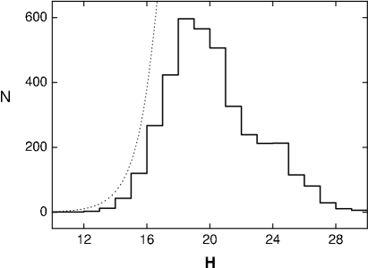
Figure 1: Histogram of the NEO population known by Jan. 5, 2006, versus the Stuart and Binzel (2004) model (dashed curve).

This paper is focused on the population of very small NEOs, up to 10 m in diameter and their possible discoveries in the close vicinity of the Earth. This range size of NEOs is also very dangerous for life on the Earth, as their atmospheric blasts can produce substantive damage on the surface (e.g. Tunguska event in 1908). Moreover, the collisions with small objects are much more frequent than with larger asteroids.

We simulate the orbital distribution of the modeled Near Earth Asteroid population to estimate the number of close encounters with the Earth within the mean Earth-Moon (0.0026 AU) distance. In this close vicinity also a 10 m asteroid in suitable geometrical conditions can reach visual magnitude about $+14^{m}$, which represents the limit for small telescopes with a short focal length. We also propose a searching program which would be able to discover such small objects in the close Earth’s vicinity. The results from the program both positive or negative and comparison with our simulated NEAs close approaches would help to better understand a small asteroid/comets ratio on the NEO orbits.

2 The simulation of NEA population

The current known NEO population is influenced by several observational effects. Due to this fact, it is necessary to use a debiased model to estimate the real population and frequency of encounters with the Earth.

We focused our simulation only on NEAs (Near Earth Asteroids) according to Bottke et al. (2000), who used three NEA source regions, the $3:1$ mean motion resonance with Jupiter, the $\nu_{6}$ secular resonance and the intermediate Mars-crossers source. They produced the NEA debiased orbital and absolute magnitude size distributions model for $H<18$, calibrated to 910 NEAs of this size range by fitting it to a biased population of NEO discovered by Spacewatch.

We extrapolated the de-biased model of the orbital elements distribution (Bottke et al., 2000) of NEA population up to $H=28$, assuming the same delivery mechanism from the source regions for small NEAs. The orbital elements a, e, i follow Bottke et al. distributions and the angular elements (argument of perihelion, longitude of ascending node and mean anomaly) were generated randomly. To calibrate the extrapolated model, we used the NEO cumulative size distribution model according to Stuart and Binzel (2004)

$$N(<H)=10^{-3.88+0.39H}~{}~{},$$ (1)

which is a most conservative approximation, compared to other authors (Bottke et al., 2000 or Rabinowitz et al., 1994). A discrete distribution has been used for each orbital element determination. For our purpose, a small range (bins) of elements value have been chosen: $\Delta a=5\times 10^{-6}$ AU, $\Delta e=10^{-6}$, $\Delta i=2.5\times 10^{-4}$ deg, $\Delta\omega=\Delta\Omega=\Delta M=10^{-4}$ deg and for the absolute magnitude $\Delta H=10^{-2}$. The NEA $a-e$ phase space condition ($q<1.3$ AU and $Q>0.983$ AU) was applied for each generated object. Finally, we got 10 964 782 NEA simulated bodies with the orbital elements and absolute magnitude distribution (Fig. 2).

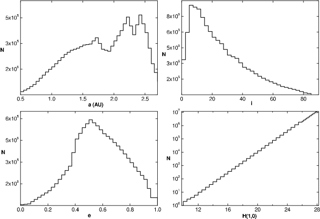
Figure 2: The semimajor axis, inclination, eccentricity and absolute magnitude (size) distributions of 10 964 782 simulated NEAs.

3 Results

We numerically integrated 10 964 782 modeled NEA orbits during one year with the aim to study geometrical conditions during their close encounters with the Earth. We were looking for very close encounters within the Moon distance (0.0026 AU) and we were also interested in all asteroids which reached visual brightness below $+14^{m}$.

In the study for a backward integration of the orbital evolution a DE multi-step procedure of Adams-Bashforth-Moulton’s type up to 12th order, with a variable step-width, developed by Shampine and Gordon (1975), was used. Input data of the positions of the Earth, the only considered perturbing body, were obtained from the Planetary and Lunar Ephemerides DE406 prepared by the Jet Propulsion Laboratory (Standish, 1998). This simple model is used due to a short time interval (one year) of integration. Several tests proved that results are consistent with all major planets incorporated. Each output file contains the Julian date, the heliocentric and geocentric distances perturbed by the Earth, the phase angle, the apparent visual magnitude, the right ascension and declination of the object.

As the main result of the one year simulation, 80 bodies inside the Moon’s orbit were obtained, which implies collisional frequency with the Earth of $2.10^{-2}$ per year. Only 18 of them also reached the visual magnitude of $+14^{m}$. As it could be expected, the cumulative number of close approaches increases approximately as a quadratic function of geocentric distance (Fig. 3). However, the count of bodies in smaller geocentric distances is higher than quadratic dependance resulting purely from Keplerian motion. It is due to the Earth’s gravity, although the effect is minor, still enough to be recognized. Moreover, the absolute magnitude distribution of the encounters within the Moon’s orbit prefers smaller objects ($<$ 100 m) with the maximum at 10 m, the most numerous objects in the NEA size distribution (Fig. 4).

The most important parameter to detect the encountered object by any searching system is its brightness. The visual magnitude distribution of approaching objects obtained from our simulation is depicted in Fig. 5. The majority of objects within Moon’s orbit reached brightnesses between $+16^{m}$ and $+18^{m}$. That is why the limiting magnitude of a small searching system would be the most restrictive factor of its efficiency.

The next important detection parameter of an object is its angular velocity in the sky. It represents the effective exposure time during which the object remains on one pixel of a CCD detector. The angular velocity of the object depends on its geocentric distance and geocentric velocity vector. The angular velocities of simulated objects within the Moon’s orbit are up to 100 arcmin/min (Fig. 6), but the most frequent velocities are in the range of $10-20$ arcmin/min.

Figure 3: Cumulative annual NEAs flux inside the Moon’s orbit (solid), theoretical quadratic dependance (dashed), D is the minimum geocentric distance. One simulated object collided with the Earth.

Figure 4: Cumulative annual NEAs flux inside the Moon’s orbit. Size distribution.

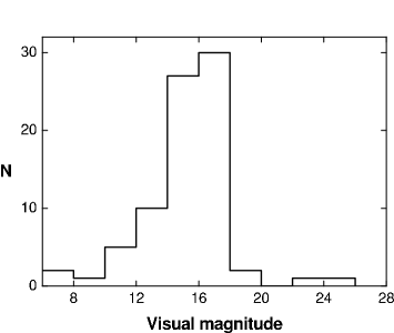
Figure 5: Annual flux of NEAs inside the Moon’s orbit and maximum visual magnitude distribution at the closest encounters.

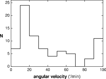
Figure 6: Histogram of angular velocity of NEAs at the closest approaches to the Earth within the Moon’s orbit.

The right plot of Fig. 7 shows all 80 close encounters trajectories within the Moon’s orbit projected on the sky in equatorial coordinates. There is no noticeable concentration toward the ecliptic. Some objects changed their positions over 100 degrees in one day. At the same time the phase angles changed very quickly, which strongly influenced the visual magnitudes of simulated objects. On the left plot of Fig. 7 there are depicted only objects inside the Moon’s orbit brighter than $+14^{m}$.

Also, there was a question how many of simulated objects could be detected by small telescopes in one year. Totally 119 bodies reached the visual magnitude of $+14^{m}$ and brighter. Just 18 of them, as we have already mentioned, were at the minimum encounter distance within the Moon’s orbit. Other bodies, mostly larger objects, reached $+14^{m}$ in greater geocentric distances at various phase angles. There are 52 of them bright enough due to their small heliocentric distances. There is a possibility to search for such objects at small elongations from the Sun (mornings and evenings) or by the LASCO coronograph on SOHO space mission.

3.1 Possible detections

We have applied several geometrical conditions and limitations on close encounters obtained from the simulation in relation to a proposed searching system with the limiting magnitude of $+14^{m}$ and weather conditions for Central Europe. In the estimate we took into account only objects with the absolute magnitude $H>19$, as we have focused on a search for small, mostly unknown objects, which would not be discovered by the current searching programs (see Fig. 1).

   

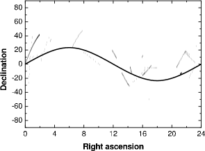
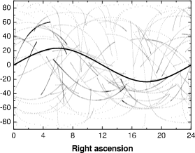
Figure 7: Close encounters trajectories within the Moon’s orbit projected on the sky. Simulated objects with the apparent magnitudes $<14^{m}$ (left) compared to all 80 NEAs inside the Moon’s orbit (right). The solid curve is the ecliptic.

The visual magnitude of an object strongly depends on the phase angle. The brightness at the phase angle $Ph=60\degr$ is about 2 magnitudes lower than that at the opposition point with $Ph=0\degr$ in the same heliocentric and geocentric distances. During a very close encounter the phase angle of the object is almost equal to its angle from the opposition point. That is why we suggest an effective search scan of the sky just within the area of $60\degr$ around the opposition. This part of the sky represents the area of approximately $10\,000\degr^{2}$. Due to our upcoming searching system limitation in the sky coverage area we suppose to cover only $\sim 2\,700\degr^{2}$, which corresponds to the phase angle $Ph=30\degr$.

The effective time which the object spends in the searching area ($30\degr$ from the opposition) reduces the probability of the detection. Another decrease occurs after reducing the magnitude of each object according to its angular velocity, which corresponds to the effective exposure time per pixel for a particular optical CCD system. There is also taken into account the time of the encounter that have to be in the nighttime for Central Europe.

Table 1: The simulation results based on the NEAs ($H<28$) population estimate by Stuart and Binzel (2004). The number of NEAs per year: (a) brighter than $+14^{m}$ with no distance limitation; (b) inside the Moon’s orbit; (c) inside the Moon’s orbit and brighter than $+14^{m}$; (d) brighter than $+14^{m}$, observable in Central Europe and $H>19$; (e) possible discoveries by the proposed searching system. Presumptive results are based on the population estimates by Bottke et al. (2000) and Rabinowitz et al. (1994).

N annually	Simulation	Bottke et al., 2000	Rabinowitz et al., 1994
a) apparent mag.$<14$	119	725	2636
b) inside Moon orbit	80	528	1920
c) inside Moon orbit and
vis. mag.$<14$	18	118	432
d) vis. mag.$<14$ and
observable in CE, $H>19$	11	66	264
e) poss. discoveries by s.s.	3	18	72

According to these conditions we obtained 18 possible detections during one year simulation for the Modra observatory (Comenius University, Bratislava, Slovakia). Only 6 of them occurred inside the Moon’s orbit. One simulated body hit the Earth. The number of bodies in suitable geometrical conditions slightly varies with a location on the Earth. The last reduction is needed due the fact that only about $20-30$ percent of the nights in Central Europe are in good weather conditions.

Finally, we obtained only $3-5$ objects, which would be detected per year with the proposed searching system for the particular weather conditions in Central Europe. This result is not very optimistic, but we have chosen for our simulation the conservative estimate of the NEA population ($H<28$) by Stuart and Binzel (2004). The total NEO population estimates up to $H<28$ by other authors like Bottke et al. (2000) or Rabinowitz et al. (1994) are several times ($6-24$ times) larger (Tab. 1).

Especially, analysis of objects inside the Moon orbit showed that a higher limiting magnitude of a wide field survey system leads to more discoveries. As it is clear from the visual magnitude distribution in Fig. 5, the $+14^{m}$ limiting magnitude is not sufficient for the effectivity of the searching system. To detect a majority of close encounters the $+18^{m}$ magnitude would be needed.

3.2 Searching system

The simulation of geometrical conditions during close approaches to the Earth were done with the aim of possible discoveries of small asteroids in the Earth’s vicinity.

An example of such a searching system is described below (Fig. 8). The parameters of the system with the CCD ST8 camera are as follows: the focal length $f=150$ mm, the aperture $D=180$ mm, the resolution of 37.15 arcsec per pixel, the field of view $5.27\degr\times 3.51\degr$, the exposure time of 30 s, which corresponds to the limiting magnitude of $+13.2^{m}$.

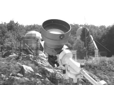
Figure 8: An example of a possible searching system for the close approaching NEOs.

The pro/-posed wide-/-field short focal length search telescope is not suitable for precise astrometric observations, but is still useful to follow up detection of close approaches. Such observation can provide a long arc with the sufficient curvature for preliminary orbit determination (Milani, 2006), afterwards confirmed by our f/5.5 60 cm reflector. This kind of detection could be classified as the original discovery.

The searching system is not finished yet and is in an early testing phase. But the most restrictive factor of such a short focal length system is a low limiting magnitude. The results of our simulation showed that the effective searching system has to have the limiting magnitude up to $+18^{m}$ and would cover not less than 10 000$\degr^{2}$ per night scan rate (Fig. 5).

4 Conclusions

We have extrapolated the de-biased model of NEA orbital distribution (Bottke et al., 2000) up to $H=28$ and calibrated it using the NEO cumulative size distribution model of Stuart and Binzel (2004). We have numerically studied of about 11 millions generated NEAs during one year. As the main result from the simulation we obtained 80 close encounters with the Earth within the Moon’s orbit. Only 18 of these objects reached the visual magnitude of $+14^{m}$.

The proposed wide-field short focal length survey system, assuming a ground-based restrictions, observational selection effects and atmospherical conditions could find several ($\sim 3$) NEAs per year. If the real population is larger (Rabinowitz et al., 1994; Bottke et al., 2000), there is a possibility to find $18-72$ objects per year. An increase of the limiting magnitude of the survey system to $+18^{m}$ with preserving a wide field of view could lead to more discoveries.

An alternative way to compare our simulation results with observations is to calculate an Earth’s annual collisional frequency. The collisional frequency of 10 m objects calculated from DoD satellite (U.S. Department of Defence) observations of large bolides is $10^{-1}$ (Brown et al., 2002). Our simulation resulted in the collisional frequency of $2.10^{-2}$ per year, which implies that the real population should be at least 5 times more numerous than that used in our expanded model up to $H=28$ based on Stuart and Binzel (2004).

- [1] \articleBottke, W.F., Jedicke, R., Morbidelli, A., Petit, J. M., Gladman, B.2000Science2882190
- [2] \articleBrown, P., Spalding, R.E., ReVelle, D.O., Tagliaferri, E., Worden, S.P.2002Nature420294
- [3] Milani, A.: 2006, personal communication. \inproceedingsRabinowitz, D.L., Bowell, E., Shoemaker, E.M., Muionen, K. 1994 Hazard Due to Comets and Asteroids T. Gehrels The University of Arizona PressTucson285 \bookShampine, L.F., Gordon, M.K.1975Computer Solution of Ordinary Differential EquationsFreeman and Comp.San Francisco
- [4] Standish, E.M: 1998, JPL IOM 312.F - 98 - 048 \articleStuart, J.S., Binzel, R.P.2004Icarus170295 \articleTóth, J., Kornoš, L.2002Acta Astron. Et Geophys. Univ. ComenianaeXXIV61