The Effect of Line of Sight Temperature Variation and Noise on Dust Continuum Observations
Abstract
We investigate the effect of line of sight temperature variations and noise on two commonly used methods to determine dust properties from dust continuum observations of dense cores. One method employs a direct fit to a modified blackbody SED; the other involves a comparison of flux ratios to an analytical prediction. Fitting fluxes near the SED peak produces inaccurate temperature and dust spectral index estimates due to the line of sight temperature (and density) variations. Longer wavelength fluxes in the Rayleigh-Jeans part of the spectrum ( 600 µm for typical cores) may more accurately recover the spectral index, but both methods are very sensitive to noise. The temperature estimate approaches the density weighted temperature, or “column temperature,” of the source as short wavelength fluxes are excluded. An inverse temperature - spectral index correlation naturally results from SED fitting, due to the inaccurate isothermal assumption, as well as noise uncertainties. We show that above some “threshold” temperature, the temperatures estimated through the flux ratio method can be highly inaccurate. In general, observations with widely separated wavelengths, and including shorter wavelengths, result in higher threshold temperatures; such observations thus allow for more accurate temperature estimates of sources with temperatures less than the threshold temperature. When only three fluxes are available, a constrained fit, where the spectral index is fixed, produces less scatter in the temperature estimate when compared to the estimate from the flux ratio method.
1 Introduction
Some of the coolest regions in molecular clouds are dense, starless cores. These dust enshrouded objects are often in the process of forming one (or a few) protostar(s) (Benson & Myers, 1989). Determining the physical properties of cores, such as temperature, composition, and density, is necessary for a complete understanding of the environmental conditions prior to the formation of a star or protostar. There has been much progress in the study of cores containing central protostars, including the success of theory in explaining the variety of emergent spectral energy distributions (SED) as an evolutionary sequence (e.g. Adams et al., 1987; Lada, 1987; Andre et al., 1993). On the other hand, the structure and evolution of cores that have yet to form a central protostar is not as well understood, and is thus an active area in current star formation research.
Dust presents one avenue to observationally investigate starless cores. Dust is prevalent in the ISM, and it is responsible for most of the extinction of starlight. For cores positioned in front of sources of known luminosity or color, the level of extinction can be an indicator of the dust content in the attenuating core (Lada et al., 1994; Alves et al., 2001). Additionally, scattered light from cores surrounded by diffuse background radiation may be used to determine the dust content (Foster & Goodman, 2006). Dust can also be directly detected through its thermal emission. Since the temperatures of the cores are 15 K, the emergent continuum SED peaks in the far-infrared (FIR) or sub-millimeter wavelength regimes (see Fig. 1). Ground and space based observations by SCUBA, MAMBO, Bolocam, 2MASS, IRAS, ISO and Spitzer have detected dust emission from many environments, and they have provided much information about starless cores (e.g. Ward-Thompson et al., 2002; Schnee et al., 2007; Kauffmann et al., 2008). The upcoming Planck and Herschel missions, which are capable of FIR observations, are also well suited for detecting dust emission. Thus, a thorough consideration of the nature of dust continuum emission, and the uncertainty associated with measuring it, is timely.
The main characteristics of the dust that determine the form of the emergent SED are the column density, temperature, and emissivity. Observationally quantifying these characteristics should constrain models of dense starless cores. Radial density profiles are often compared with a stable isothermal Bonnor-Ebert sphere (Bonnor, 1956; Ebert, 1955), for which the volume density is constant near the center, but drops as at larger radii (e.g. Bacmann et al., 2000; Schnee & Goodman, 2005). The density gradients may vary from core to core, which in turn may (or may not) be due to an evolutionary sequence as cores continually collapse to form a protostar.
Though gas temperatures in a stable Bonnor-Ebert sphere are constant, theoretical results have suggested that dust temperatures decrease towards the center to values as low as 7 K (e.g. Leung, 1975; Evans et al., 2001; Zucconi et al., 2001). And, recent observational investigations have in fact identified cores with such gradients in the dust temperatures (e.g. Schnee et al., 2007; Ward-Thompson et al., 2002). Though the dust mass is only a fraction of the gas mass ( 1/100), gas temperatures may also exhibit gradients, due to the coupling between dust and gas at high enough densities (Goldsmith, 2001; Crapsi et al., 2007). The (recent and upcoming) availability of higher quality observational data will require a thorough interpretation of emergent SEDs to accurately assess the temperature, as well as density, profiles of the observed sources.
The common assumption is that the emergent SED from interstellar dust is similar to the Planck function of a blackbody, modified by a power-law dependence on the frequency (Hildebrand, 1983). The spectral index of the dust emissivity power-law, , is dependent on the bulk and surface properties of the dust grains. As shown by Keene et al. (1980), observations limited by sparse flux sampling may be consistent with various SEDs described by different values of . A precise estimate of the value of is necessary to accurately derive other properties of the observed source, such as the temperature and the mass of a cold core. The emissivity-modified blackbody spectrum is the basis for many analyses of dust properties in observed cores (e.g Kramer et al., 2003; Schnee et al., 2005; Ward-Thompson et al., 2002; Kirk et al., 2007).
Dupac and coworkers fit observed FIR and sub-millimeter fluxes with a modified blackbody spectrum, and they suggested that decreases with increasing temperatures, from 2 in cold regions to 0.8 - 1.6 in warmer regions ( 35 - 80 K; Dupac et al., 2001, 2002, 2003). Such analyses may be sensitive to the simplified assumption of a constant temperature along the line of sight. Using radiative transfer calculations of embedded sources, Doty & Leung (1994) demonstrated that the accuracy of the parameters estimated from measured fluxes is sensitive to the precise nature of the source (e.g. opacity, temperature distribution); they found that the Rayleigh-Jeans (R-J) regime of the emergent spectrum is better suited for an accurate determination of the dust spectral index. Doty & Palotti (2002) found that the use of flux ratios to estimate the spectral index is sensitive to which wavelengths (of the given fluxes) are used in the ratio; they also found that is more accurately determined when fluxes at longer wavelengths are used in a fit. Schnee et al. (2006) also showed that various ratios of fluxes (with different wavelengths) give different estimates for dust temperature and column density, due to an inaccurate isothermal assumption.
Here, we systematically investigate how line of sight density and temperature variations, similar to those in dense cores, as well as noise uncertainties, affect the temperature and spectral index estimated from IR and sub-millimeter observations. We focus on two commonly employed methods. The first method uses a direct fit of a modified blackbody SED. For the second method, ratios of the fluxes are used to determine the temperature and from an analytical prediction. Both methods usually rely upon an assumption of constant temperature along the line of sight. Using simple radiative transfer calculations of model sources, and Monte Carlo experiments, we assess how well the resulting temperature and spectral index estimates recover properties of known input sources.
This paper is organized as follows. In the next section (2), we present the analytical expression of the power-law modified blackbody spectrum, and briefly introduce two well known methods used to estimate the dust properties from IR and sub-millimeter continuum observations. In our analysis of the two methods, we consider numerous scenarios typical of observations of star forming regions. Table 1 shows the particular scenario considered in each subsection, and may be used as a brief guide to 3 - 6. We begin our analysis by considering non-isothermal sources in the ideal limit where a large range of fluxes at different wavelengths are available for fitting an SED. We then systematically exclude fluxes, culminating with the scenario where only a few fluxes are available, in which case the flux ratio method is employed. Throughout our analysis, we also consider the effect of noise in the observations, of both isothermal and non-isothermal sources. In 3, we describe the method to estimate source temperatures using direct SED fitting; we investigate how line of sight variations, noise, and the sampling of different regions of the emergent SED affect the resulting temperature estimates. We also discuss our findings in the context of recent published works. In the following section (4) we analyze the flux ratio method focusing on the effect of noise, through the use Monte Carlo simulations. We then compare the two methods using a radiative transfer simulation to model the emission from an isolated starless core in 5. After a discussion in 6, we summarize our findings in 7.
2 Dust Emission: Common Assumptions and Methods
2.1 Isothermal Sources
The emergent continuum SED due to dust is often expressed analytically as the product of a blackbody spectrum at the dust temperature and the frequency dependent dust opacity . The observed flux density associated with this SED takes the form
| (1) |
where is the solid angle of the observing beam, and is the column density of the emitting material. The opacity is empirically determined to have a power law dependence on the frequency (Hildebrand, 1983):
| (2) |
The spectral index depends on the physical and chemical properties of the dust. For silicate and graphite dust composition common in much of the ISM, (Draine & Lee, 1984). However, observations have shown that can reach values as low as 1 and as high as 3 in various environments (e.g. Oldham et al., 1994; Kuan et al., 1996; Mathis, 1990). Indeed, the spectral index is a key parameter and accurately determining its value, along with the column density and the temperature , is crucial for a thorough description of dust properties in an observed region. Those are the three parameters that are required to accurately describe an observed flux density (per beam, i.e. ).
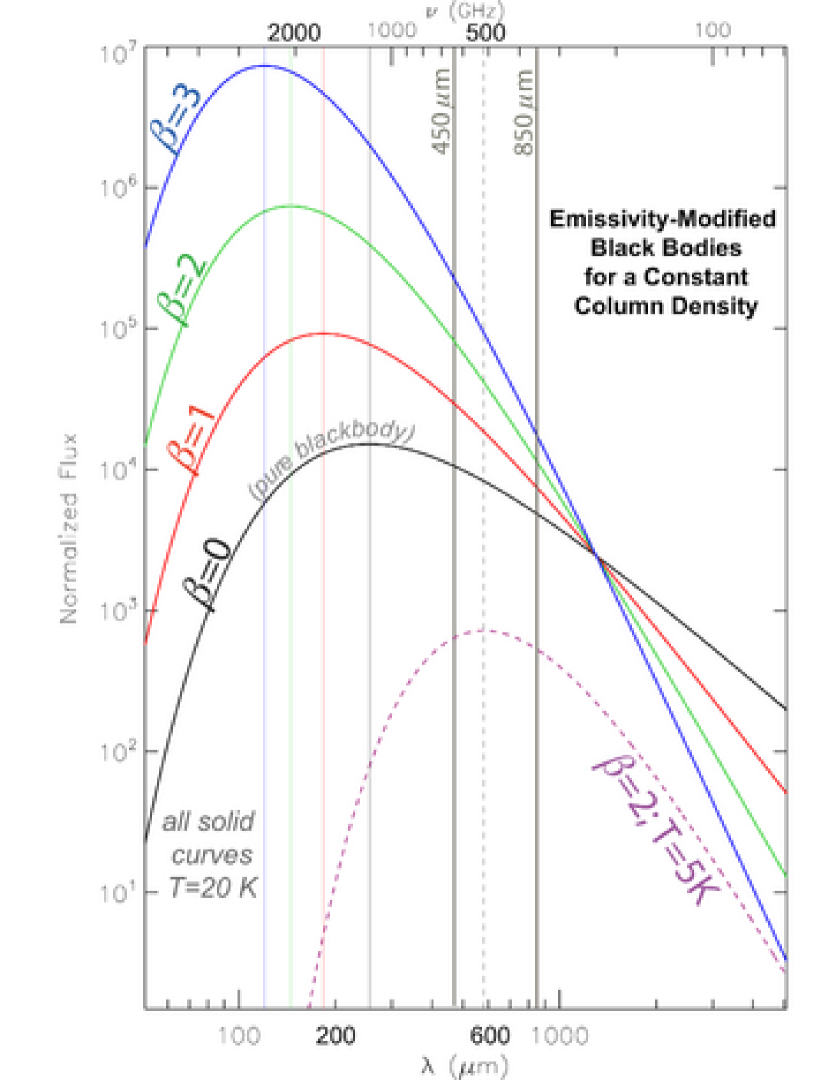
Figure 1 shows SEDs from a 20 K source with different values of , but constant column densities. For comparison, the SED from a 5 K source with the same column density and = 2 is also shown. The SEDs are all calibrated using an equivalent = , which is why all the 20 K SEDs intersect at 230 GHz. Sources with higher spectral indices () produce SEDs with steeper slopes at long wavelengths (in the R-J regime), increasing peak fluxes, and shorter peak wavelengths. Similar to Wien’s Law for a pure blackbody, for a given value of , a modified Wien’s Law indicating the wavelength corresponding to the peak in , , can be determined numerically.111This modified Wien’s Law gives the wavelength that corresponds to the peak in . In other texts, sometimes refers to the wavelength corresponding to the peak of . For = 2, , and for =1, . Doty & Palotti (2002) find that is a good fit for .
2.2 Non-Isothermal Sources: A Simple Example
Equations (1)-(2) describe the spectrum emitted from dust at a single temperature . For a 3D source with various dust characteristics, the emergent SED will be a combination of SEDs from all the dust in the source. For optically thin emission, the emergent SED is simply the integrated SED from each dust grain. Here, we briefly consider the effect of using equations (1)-(2) to characterize an SED from a source with two different dust populations. This relatively simple analysis is a prelude to the effect of line of sight temperature variations on commonly employed methods to estimate dust properties.
Figure 2 shows the emergent SED from a source with two populations of dust grains, along with the SED from each individual component: the temperature and column density of the cool component is = 10 K and , respectively; for the warm component, = 15 K and . Physically, such a system is similar to a 10 K dense core surrounded by a 15 diffuse envelope. The spectral indices for both components are set to = 2.
The peak of the emergent SED in Figure 2 occurs at = 251 µm. Using the modified Wien’s Law for =2, the temperature of an isothermal source that would produce a spectrum which peaks at that wavelength is 11.6 K. Though this temperature occurs somewhere between the temperatures of the two isothermal sources that contribute to the emergent SED, in practice knowledge of the peak of the SED of an unknown source is not easily determined. Further, it is not obvious how one should interpret the temperature assigned to a source which itself is not isothermal.
In subsequent sections, we assess how well emergent SEDs are described by equations (1)-(2), and what information about the source temperature can be garnered from continuum observations that span different regions of the SED. We also consider the more realistic constraint of limited sampling of the emergent SED. One question we aim to address, for instance, is whether fluxes in different parts of an emergent SED, such as the Wien or R-J regimes, are preferable for determining the dust properties.
Two commonly employed methods to determine the properties of dust from continuum observations are: (1) a direct fitting of equations (1) & (2); and (2) the use of ratios of observed flux densities at 2 or more wavelengths. For isothermal sources, and with ideal observations with no uncertainties, both methods will accurately recover , , , and . However, all sources are unlikely to be isothermal, and even the most accurate observations include some level of intrinsic noise. In the following sections, we quantify how these factors affect the accuracy of the derived parameters. After describing the two methods in further detail, we use simple numerical experiments to evaluate the accuracy of the methods in determining the dust properties from observations of star forming cores.
3 Direct SED Fitting
A minimized fit of equations (1)-(2) to a number of observed fluxes can be performed to estimate the dust properties. There are essentially three parameters to be fit, the temperature , the spectral index and the absolute scaling, which is just the product of the column density and the opacity at a given frequency . Since a fit will only produce the scaling (which is the optical depth at a particular frequency, e.g. at 230 GHz), other assumptions and/or techniques are necessary to obtain estimates of and . For example, if the opacity at a wavelength is known (e.g. for 230 GHz), then the fit can estimate directly. Extinction studies are another avenue to estimate ; the level of attenuation (usually from optical and NIR observations) due to dust in dark clouds in front of the stellar background is directly related to the column density of the dust (e.g. Lada et al., 1994). This method is advantageous since it provides an independent estimate of , but also requires assumptions, such as the ratio of total-to-selective extinction (e.g. Hildebrand, 1983; Mathis, 1990, and references therein). Further, to obtain the total column density along the line of sight, and not just that of the dust, an additional assumption of the dust-to-gas ratio is required. In our analysis, we will assume that only IR and sub-millimeter observations are available, and thus will limit our analysis to the estimation of and . Our focus here is to investigate how well a given method can reproduce temperatures and spectral indices only; estimation of the absolute column density and opacity is beyond the scope of this work.
3.1 Effect of Line of Sight Temperature Variations
3.1.1 Two-Component Sources
We begin by considering ideal (i.e. error-free) observations of simple two-component sources. Fitting experiments involving sources with two dust populations have been explored by Dupac et al. (2002); their aim was to determine the amount of cold dust, along lines of sight with warmer dust, that is necessary to reproduce the fit results of their observations. Here, we simply evaluate the resulting fits when fluxes at different wavelengths are available.
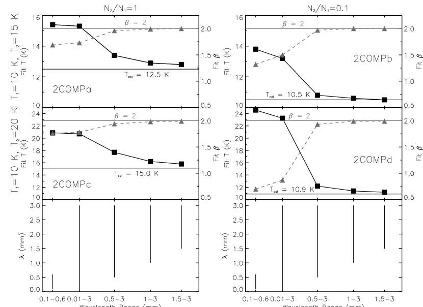
The temperatures of the cold and warm media are and , respectively, and the column density ratio is . Such systems are analogous to isothermal (spherical) dense cores surrounded by warmer envelopes. Modified blackbody SEDs (eqns. [1]-[2]) are constructed for the two media, both with = 2. A particular example SED of this general case is shown in Figure 2. We then fit equation (1) to the integrated SEDs, solving for and (as well as the scaling factor ). Figure 3 shows the fit temperatures and spectral indices from observations of a variety of two-component systems, along with the wavelength range of the fluxes considered in the fit.
Since varies along the line of sight, the best fit will likely not be equal to the temperature of one of the two sources. One characteristic temperature of this two-component medium is the density weighted temperature (e.g. Doty & Palotti, 2002). Since this density weighted temperature is analogous to the column density, we will call it the “column temperature,” . The estimated temperature from a fit can be compared with this true column temperature.
As shown in Figure 3, the best fit temperature is systematically too high when all fluxes at (integer) wavelengths between 10 - 3000 µm are considered in the fit. In fact, when the temperature difference between the two components is large, the best fit temperature is actually larger than the warmer medium, as in “2COMPc” and “2COMPd,” lines of sight containing dust at 10 and 20 K. Further, when all wavelengths are considered, the fit value of is always lower than the actual value of 2. However, when shorter wavelengths are systematically excluded from the fit, the best fit temperature decreases and approaches the column temperature. The best fit also approaches the model value of 2 when fluxes in the R-J wavelength regime are the only ones used in the fit, consistent with the findings of Doty & Leung (1994). In practice, for deriving dust properties from the emergent SED, it may be necessary to exclude fluxes with 100 µm due to the contribution of embedded sources as well as transiently heated very small grains (Li & Draine, 2001), depending on the environment.
3.1.2 Cores with Density and Temperature Gradients
Recent theoretical and observational studies have indicated that the dust temperature in starless cores decreases toward the center, reaching low values 7 K (e.g. Evans et al., 2001; Crapsi et al., 2007; Schnee et al., 2007; Ward-Thompson et al., 2002). We thus investigate the emergent SED from cores containing temperature gradients like those observed, and whether any useful information can be obtained from fitting a single power-law modified blackbody spectrum to that SED.
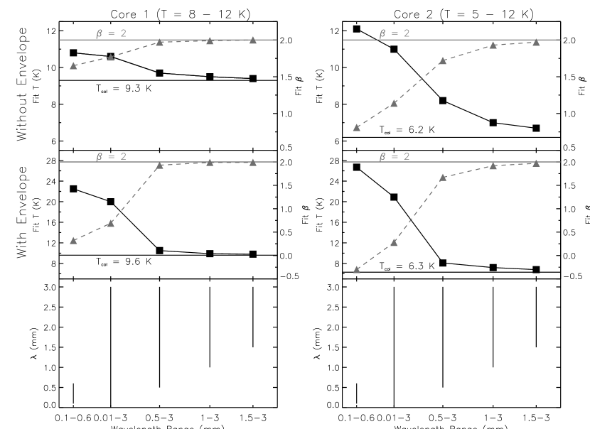
To construct the model cores, we use the density and dust temperature profiles presented by Evans et al. (2001), who performed radiative transfer simulations on a variety of model cores with a range of density profiles. Though the resulting dust temperature profiles are sensitive to the model density profiles, the relationship between and column density is relatively uniform between models with different (volume) density profiles (see Fig. 9 of Evans et al., 2001). In our analysis of emergent SEDs from starless cores, we construct two cores, with temperatures ranging between 8 - 12 K and 5 - 12 K; the column densities are as indicated in Figure 9 of Evans et al. (2001): increases with decreasing temperature (and thus with decreasing core radius). At the outer edge of the core, at a temperature of 12 K, the column density is set to 2 cm-2; the temperature drops to 8 K in model Core 1 and to 5 K in model Core 2, with column densities of 1.25 cm-2 and 1 cm-2, respectively. Besides these isolated cores, without any surrounding medium, we also consider cases where the cores are surrounded by an envelope with a temperature of 20 K and a column density of 1 cm-2.
As described in 3.1.1 we begin by fitting the emergent SED assuming that fluxes at various wavelength ranges are available. Figure 4 shows the resulting best fit temperatures and spectral indices for the two cores. The SEDs from the cores without an envelope are analogous to an SED obtained by accurately subtracting off flux due to larger scale emission from the surrounding region, or an SED from a truly isolated core. When equation (1) is fit to fluxes at 100 - 600 µm, the best fit temperature is 3 K ( 15%) off from the column temperature of Core 1, but differs from the column temperature of Core 2 by 6 K ( 50%). The best fit spectral index also shows large variation between the two cores. For Core 1 ( K) the fit of 1.65 is within 20% of the model value of 2. However, for Core 2 ( K), the best fit of 0.81 is erroneous by over a factor of 2. As more short wavelength fluxes (in the Wien regime) are excluded, the fits recover the model spectral index more accurately; the temperature estimate also decreases, approaching the column temperature of the core.
When the core is surrounded by a warmer envelope, or when the flux from extended regions has not been properly accounted for, then the discrepancy between the best fit parameters and the core properties increases, as expected. For Core 2, a fit to the fluxes at 100 - 600 µm results in an estimate for with an unphysical sign (-0.3). Including the envelope, the discrepancy between the fit and the column temperature at short wavelength fluxes increases by 50%, compared with the cores without the envelope.
We performed such fits for cores surrounded by more diffuse envelopes, with a column density that is a factor 10 - 100 times lower than that of the core (1 cm-2). Such envelopes only have a slight effect on the fit temperatures, because the column temperatures are not significantly different compared to the isolated cores. The envelope does have an appreciable effect on the best fit when fluxes near the peak of the SED are considered in the fit. However, excluding short wavelength fluxes still recovers the true spectral index reasonably accurately, as Figure 1 would suggest.
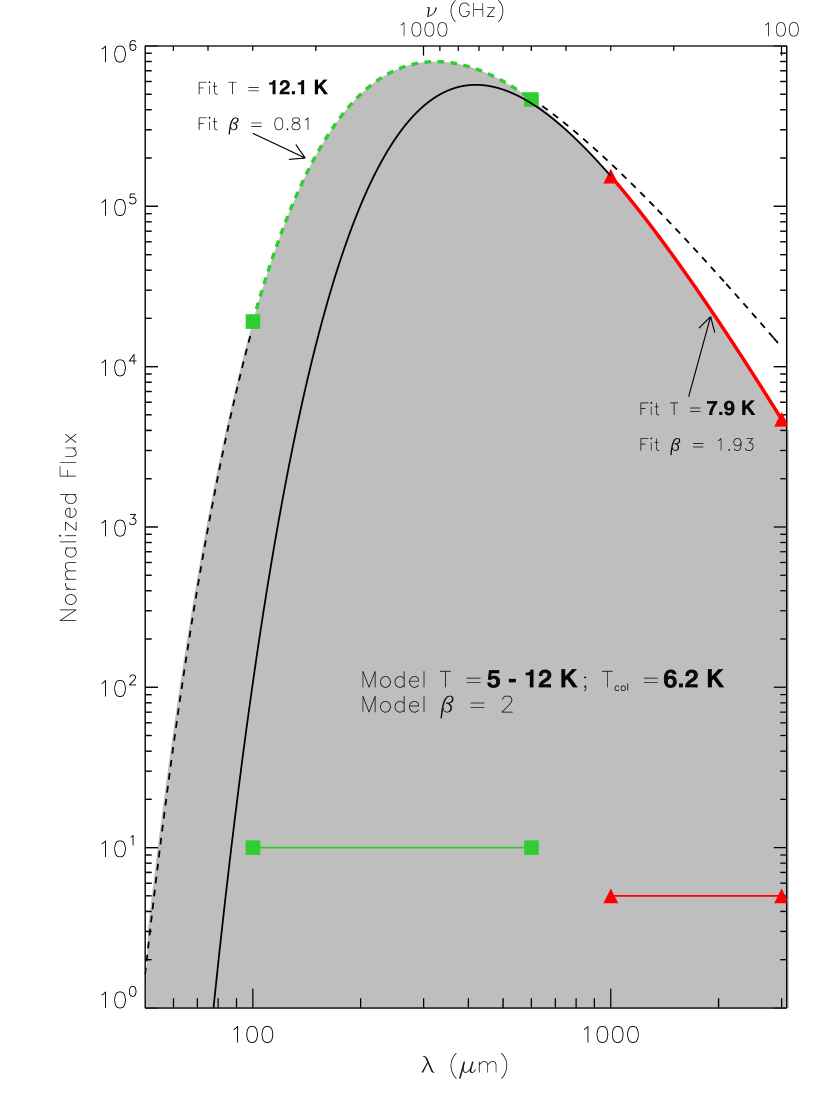
Figure 5 shows the emergent SED from Core 2 ( 5-12 K) without an envelope, along with the results from two fits, one to the fluxes from 100 - 600 µm, and the other to fluxes from 1 - 3 mm. The fit at shorter wavelengths does indeed reproduce the peak and shorter wavelength fluxes of the emergent SED reasonably well, but severely overestimates the fluxes at longer wavelengths. On the other hand, the fit to long wavelength observation reproduces the R-J tail of the spectrum accurately, but underestimates the fluxes at all shorter wavelengths.
The peak of the emergent SED from Core 2 occurs at = 324 µm. From the modified Wien’s Law (for =2) , the temperature associated with this wavelength is 8.9 K. This value is closer to the maximum temperature, 12 K, of the source, than the column temperature =6.2 K. In this case, is dominated by the high density, cold center, whereas the peak of the SED is primarily influenced by the warmer, low density regions of the core. Since the SED has an exponential dependence on the temperature in the Wien regime, which, for such a cold core, goes up to 100 µm, even low density regions may dominate the total SED emerging from a region, due to the higher temperatures.
3.1.3 Summary of the Effect of Line of Sight Temperature Variations
As expected, the emergent SED at wavelengths near the peak is poorly described by a simple power-law-modified-blackbody, due to temperature variations along the line of sight, as previously documented in the literature (e.g. Doty & Palotti, 2002; Schnee et al., 2006). Nevertheless, the fits can still reveal properties of the observed source, namely that the best fit temperature approaches the column temperature and the best fit approaches the model value as shorter wavelengths are excluded. There are also other revealing trends that warrant further investigation. First, the systematic exclusion of short wavelength fluxes results in different and estimates; for an isothermal source, the fit would always be the same (and equal to the temperature of the source). If this trend also occurs when there are only a few observations, then short wavelength observations can still be used to determine whether a source is isothermal or not. Second, there also appears to be an inverse - relationship: whenever is overestimated, is underestimated. A similar relationship has been discussed by Dupac and coworkers using observations at wavelengths 600 µm (Dupac et al., 2001, 2002, 2003). A thorough analysis of the sources observed by Dupac et al. would be warranted to rule out that the inferred anti-correlation is simply due to line of sight effects. As we discuss in the next section (3.2), an inverse - trend may also arise from SED fits due solely to noise in the observations.
3.2 Effect of Noise
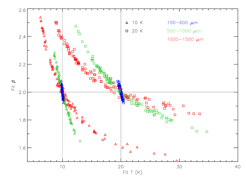
Uncertainties in observed fluxes may also lead to incorrect temperature and spectral index estimates from SED fitting. To assess the effect of noise, we first consider fluxes from isothermal sources with modest 5% uncertainties in each observed flux. A number fluxes from a range of (integer) wavelengths are considered in the fit: 100 - 600 µm, 500 - 1000 µm, and 1000 - 1500 µm. In these Monte-Carlo experiments, each flux is modified by a random value drawn from a Gaussian distribution, with = 0.05.
Figure 6 shows the best fit and estimates for isothermal sources, one with = 10 K and =2, and the other with = 20 K and =2. Each set of noisy fluxes, spanning the different wavelength regimes, is generated 100 times; a modified blackbody is then fit to each set. As expected, there is a spread in the best fit and .
Fits from both the 10 K and 20 K source show little scatter when only fluxes with wavelengths 100 - 600 µm are considered in the fit, suggesting that an SED is not very sensitive to noise in the Wien regime. However, at longer wavelengths, there is a large spread in the estimated and . Including fluxes between 500 - 1000 µm, the fits from the 10 K source give - 2.3 (within 20% of the source value) and 8 - 14 (within 40%). This range increases when including fluxes between 1000 - 1500 µm: (within 30%) and (within only 200%). That the longer wavelength fits show more scatter is not unexpected given the shape of an SED (see Fig. [1]).
In the R-J tail, the SEDs from sources with different temperatures are similar in shape, since the slope is determined primarily by (see Fig. [1]). Thus, small errors in the observed fluxes may result in inaccurate (and thus ) fits. At shorter wavelengths, largely determines the shape of the SED, so small uncertainties may be insufficient to significantly alter the temperature that best matches the observation in a fit. For the 20 K source in Figure 6, there is less of a difference between the spread in and for the fits to 500 - 1000 µm and 1000 - 1500 µm fluxes. This occurs because at 20 K, the range spanning the shorter wavelengths (500 - 1000 µm) is already well enough into the R-J region of the spectrum (see Fig. [1]), so the fit is already very sensitive to noise.
The clear inverse - trend that emerges from SED fits to noisy fluxes is similar to the trends found from fits to noise-free fluxes from non-isothermal sources (as suggested by Figs. 3 and 4). Apparently, whenever a fit underestimates the temperatures, the spectral index is overestimated, and vice versa. This effect is amplified when noisy fluxes in the R-J regime of the spectrum are considered in the fit, and can be understood when comparing SEDs with different values of . Consider a 20 K isothermal source, with = 2, shown in Figure 1. Assume the source is observed at various wavelengths, primarily at 1 mm, but that the peak is also sampled. Further, assume the noise level in the fluxes is such that the least squares fit preferentially obtains a of 1. The peak of the SED with = 1 in Figure 1 occurs at longer wavelength than the peak of the = 2 SED, and so a fit = 20 K, with , would not reproduce the peak of the observed SED well. In order for the fit to reproduce the peak of the SED from the 20 K source, but with a best fit of 1, the best fit must be held at a larger value than 20 K. In general, therefore, when a fit underestimates , is overestimated.
We have shown that an inverse correlation between and can occur due to an incorrect assumption of isothermality, or due to intrinsic noise in the observations. Such a trend would of course also occur for noisy observations of non-isothermal sources. We discuss the combination of noise and line of sight temperature variations when we discuss the additional limitation of including only a small number of fluxes in 3.4.
3.3 Estimating and with Sparse Wavelength Coverages
The fitting experiments indicate that, for lines of sight with starless-core-like temperature and density gradients, the resulting fits produce lower temperatures and higher spectral indices as shorter wavelength fluxes are excluded in the fit. In all our tests so far, we have included all wavelengths within a given range. In practice, however, obtaining only a (small) number of observations at different wavelengths of a source is typically feasible. Current (e.g.Spitzer, SCUBA, Bolocam, MAMBO) and near future observations (e.g. Herschel and Planck) can provide fluxes at a number of FIR and sub-millimeter wavelengths. However, many of those wavebands provide fluxes at or near the peak of the integrated SEDs of dense cores. Thus, SED fitting may not provide accurate estimates of the (column) temperature and spectral index. Yet, determining whether or not a core contains temperature variations is instructive in itself. Further, the temperature obtained from a fit to long wavelength fluxes can be deemed the upper limit of the coldest region within the core. We thus investigate whether the identification of temperature variations along the line of sight, as well as an accurate estimate of the temperature limit, are still feasible when a small number of fluxes, including those with wavelengths near the peak of the SED, is used in the fit. We begin by describing the effect of fitting an SED to a limited number of noise-free fluxes. After that, we consider the effect of noise in observations of sources with temperature variations, in 3.4.
We construct another optically thin 2 component medium, with = 10 K, = 15 K, = 0.02, and =2, similar to “2COMPb” in Figure 3, but with a greater density contrast. We perform a fit assuming fluxes were obtained at 60, 100, 200, 260, 360, and 580 µm. The reason we choose these particular parameters, which are realistic for innermost and outermost regions of a core, is to assess whether any patterns emerge from fitting different fluxes from a source with only slight temperature variations. We choose fluxes at wavelengths near the peak for more direct comparisons with real observations of cores. The column of panels in Figure 7(a) shows the fitting results. The bottom panel of Figure 7(a) indicates the observed wavelengths, along with the emergent SED from the 2 component source. There are no significant differences in the fitting results when excluding the 60 µm flux. However, when the additional flux at 100 µm is excluded, the best fit temperature decreases and spectral index increases. We were unable to obtain a good fit with only three fluxes; we have found that a minimum of four wavelengths is necessary to obtain a fit with three free parameters.222As we discuss in 5, a good fit can be found with only three data points if one (or more) of the fit parameters (, , or ) is held fixed.
Excluding short wavelength fluxes, even with a limited number of observations in the Wien regime, results in a lower estimate of and a higher estimate of . We found the same trend regardless of what wavelengths were considered in the fit, and for a variety of systems with an inverse relationship between the column density and temperature.
3.4 Implications to Recent Observations
We now perform a similar tests to published observations of cold star forming regions, beginning with the observations presented by Stepnik et al. (2003). They analyzed a filament in the Taurus molecular cloud using 60, 100, 200, 260, 360, and 580 µm fluxes observed from IRAS and the balloon borne experiment PRONAOS/SPM. After subtracting off emission attributed to the surrounding envelope, they fit the 6 data points to obtain an estimate of the temperature and spectral index of the filament. We carry out the exact same procedure, but also perform fits excluding the short wavelength fluxes. The fitting results are shown in Figure 7(b). As with the two-component model shown in Figure 7(a), the exclusion of the 60 µm flux does not alter the fit. However, additionally excluding the 100 µm flux decreases the fit by 1 K, and increases from 1.98 to 2.13. This variation is rather similar to the simple 2 component fit, indicating that there might be a temperature variation within the filament, and that the actual value of the spectral index is greater than 2.1 (if the spectral index itself is constant in the filament). A value of 11.13 1.29 K can be assigned as an upper limit for the column temperature of the filament. The interpretation of a temperature variation within the filament cannot be definitive, however, due to the large uncertainties. Within the uncertainties, the fit and are constant regardless of which fluxes are considered in the fit. More observations, preferably at longer wavelengths, are necessary to confidently determine whether there are temperature variations within the filament itself, and for an accurate estimate of the spectral index.
Kirk et al. (2007) also employed SED fitting to Spitzer and ISO observations to estimate the temperatures of numerous cores. We analyze their fluxes in a similar fashion. Though a few of the cores did not show definitive temperature drop as shorter wavelength fluxes were excluded, the well studied core B68 shows a clear drop in temperature and an increase in the spectral index after short wavelength fluxes are excluded. The fitting results for B68 is shown in Figure 7(c).333Using all 7 of their fluxes, Kirk et al. (2007) obtain a best fit =12.5 K; the difference between their value and ours arises because they kept at a fixed value of 2. Our results agree when is fixed at that value in our fits. The best fit temperatures decreases by 5 K when the 70 and 90 µm fluxes are excluded in the fit. There is an additional 1 K temperature drop when the 160 µm flux is excluded. There is also a corresponding increase in from 1.2 to 2.4. One interpretation of such a high spectral index is that the dust grains are covered by icy mantles (e.g. Kuan et al., 1996); this interpretation would be reasonable for B68, where there is significant molecular depletion onto dust grains (Bergin et al., 2002). The variations in the spectral index and temperature estimates when short wavelength fluxes are excluded in the fit, along with the relatively small error bars, strongly suggests that there are dust temperature (and corresponding inverse density) variations within B68. We thus assign an upper limit of 10.8 0.1 K for the coldest region within B68. Our fits also suggest that the spectral index of dust in B68 2.4, if that property is constant throughout the core.
We perform the same test of the data presented by Dupac et al. (2001). They estimated the temperature and spectral indices of regions in the Orion complex. One of the regions appears to be a dense core without a central source, referred to as “Cloud 2” by Dupac et al. (2001). Figure 7(d) shows our fitting results. For this core, longer wavelength data at 1.2 and 2.1 mm are available. In this case, the exclusion of short wavelength data reduces the temperature by 2 K. The spectral index also increases, from 2.2 to 2.5. These results are also suggestive of temperature variations within the core, but due to the relatively large uncertainties, an isothermal description cannot be ruled out.
We have found that the systematic exclusion of short wavelength data for dense cores results in lower best fit temperatures, and higher best fit spectral indices. A trend of decreasing with increasing has been put forward as a physical property of dust grains in the ISM by Dupac et al. (2003). They find such a trend by fitting equation (1) to observed fluxes primarily from PRONAOS/SPM, corresponding to wavelengths (in the range 100 - 600 µm) near the peak of the SEDs emitted by dust. Dupac et al. (2003) argue that line of sight temperature variations only result in a slight variation of with , and that unrealistically high density contrasts ( 100 ) are necessary to reproduce the magnitude of the inverse - correlation (see also Dupac et al., 2002). We find that temperature variations in realistic cores with a uniform spectral index would show an inverse - relationship when observed at wavelengths near the peak of the emergent SED. Besides resulting in erroneous estimates, the best fit parameters vary as short wavelength fluxes are excluded in the fit, with the best fit approaching the correct value when only long wavelengths are considered. Further, we also find that modest errors, as low as 5%, in observed fluxes from isothermal sources lead to erroneous and estimates. The trend in the points in a - plane from a number of fits to noisy fluxes also show such an inverse correlation (Fig. [6]). It would thus be informative to compare the form of the - relationship we find with that of Dupac et al. (2003). We note that though we only consider objects with 20 K in this work, we investigate the derived inverse - relationship due to noise in observations of isothermal sources with temperatures up to 100 K in an accompanying paper (Shetty et al., 2009).
3.4.1 A True Inverse - Correlation?
To further investigate the derived inverse - correlations, we again consider the two-component medium “2COMPd,” with temperatures = 10 K, = 20 K, and a column density ratio = 0.1. As shown in Figure 3, a modified blackbody SED fit results in a estimate of 23.3 K and a estimate of 0.23, using fluxes measured between 10 - 3000 µm. To compare with realistic observations, we perform the fit to data sets each containing fluxes at 5 wavelengths. Two sets of wavelengths are considered: one with fluxes near the peak of the SED at 100, 200, 260, 360, and 580 µm, and the other with fluxes in the R-J tail of the SED at 850, 1100, 1200, 1500, and 2100 µm. In order to account for the effect of a 5% uncertainty in the observations, due to noise or calibration errors, for example, each flux is multiplied by a random value drawn from a Gaussian distribution with a mean of 1.0 and dispersion of 0.05. We generate 100 sets of fluxes in this manner, and fit equation 1 to each set of fluxes, as in the numerical experiments of isothermal sources presented in 3.2.
Figure 8 shows the fitting results from these simulated observations. The fits to the observed fluxes at long wavelengths show a scatter in the - relation, due to the uncertainties in the fluxes. The fits at shorter wavelengths do not show as much scatter, but the best fit and are very poor estimates of the true or the column temperature of 10.9 K. As previously discussed, this inaccuracy at short wavelengths results because the emergent SED from a non-isothermal source is not well fit by a single power law modified blackbody spectrum.
Dupac et al. (2003) observe a variety of sources, including dense cores as well as much warmer sources. After fitting modified blackbody SEDs to the observed fluxes, with wavelengths 600 µm, they find that a hyperbolic form in represents the fits well. They investigated the effect of noise in a model with a range of uncorrelated - pairs, and concluded that such a model is inconsistent with the observed data. The shape of the - correlation in Figure 8 from a model with a single is remarkably similar to that shown in Dupac et al. (2003). This suggests that an inverse, and possibly even hyperbolic-shaped, - relationship is not necessarily due to real variations in the dust spectral index with dust temperature. The relationship may simply be due to temperature variations along the line of sight, along with uncertainties in the observed fluxes. At the short wavelengths considered by Dupac et al. (2003), for the warmer sources the observed wavelengths may indeed fall in the R-J part of the spectrum. For these sources, the “short wavelength” fits will be analogous to the “long wavelength” set in Figure 8. For sources that are dense cores, if they are not isothermal, the SEDs at those short wavelengths are not well fit by equation (1); a fit would produce a large estimate, relative to the column temperature, and would underestimate .
For isothermal sources (3.2), the addition of noise to the observed fluxes further degrades the parameter estimates. Our analysis indicates that the SED fits to fluxes with 600 µm from various warm isothermal sources with 60 K may all produce similar and estimates (Shetty et al., 2009). Uncertainties in the observed fluxes of starless cores may be responsible for some of the scatter in the - diagram shown by Dupac et al. (2003). However, all of the spread is likely not a consequence solely of noise, since Dupac et al. (2003) observe a variety of sources. One possibility is that the spectral index varies within a source, which is a situation we do not model (see Table 1). The emergent SED from such sources will of course be more complicated, for which alternative analysis techniques may provide better parameter estimates. We note that the points in Figure 8 would simply be systematically offset had we considered a source with a different (constant) spectral index from = 2 (Shetty et al., 2009). Thus, had we included multiple sources with different (constant) values of , the - diagram would be further populated. Though we cannot exclude the possibility that the spectral index of dust decreases with increasing temperature, we have shown that simple power-law-modified-blackbody fits to observed data can result in misleading - relationships which appear like those sometimes claimed to be of physical origin.
We have demonstrated that the assumption of isothermality can lead to significant errors in estimates of and from SED fits. Noise contributes to additional uncertainty in the estimated parameters. In the next section, we describe the effect of noise on a different method commonly used to estimate and , by means of flux ratios, focusing on isothermal sources. We then compare the flux ratio estimates to those derived from SED fitting for sources with line of sight temperature variations.
4 Flux Ratios
An alternative to full SED fitting for estimating the temperature is through the use of ratios of observed fluxes. For a given observation, the known quantities in equation (1) are the flux density and the beam size . With two observations (smoothed to a uniform resolution) at different frequencies , corresponding to wavelengths , the ratio of produces an equation where the two unknown quantities are and :
| (3) |
where . The main assumptions made to derive this equation are that and are constant along the line of sight. If is known a priori (or otherwise assumed to be known), then equation (3) can be used to estimate the temperature from only two observations (e.g. Kramer et al., 2003; Schnee & Goodman, 2005; Ward-Thompson et al., 2002; Schlegel et al., 1998).
Including a third observation at frequency , corresponding to wavelength , taking ratios using all three flux densities produces
| (4a) | |||
| (4b) | |||
The advantage of using this equation to estimate the temperature is that no assumption for the value of is required, though is assumed to be constant along the line of sight. A similar equation can be derived for observations at four wavelengths. However, as we discuss in 6, in that case a direct fit of equation (1) is reliable. We will hereafter refer to the left hand side of equation (4) as the “flux ratio,” and the right hand side as the “analytic prediction.”
Schnee et al. (2007) used fluxes from observations of the starless core TMC-1C at 450, 850, and 1200 m in equation (4). They found that the errors in the observations would have to be 2% in order to accurately estimate the temperature (of an isothermal source). The goal of that study, besides mapping the temperature, was also to map the spectral index and column density. Once an estimate for the temperature is obtained, the spectral index can be estimated through the use of the ratio of any two fluxes as:
| (5) |
In principle one can also estimate the column density , modulo , once and are derived from equations (4)-(5) (e.g. Schnee et al., 2006). As discussed in 3, however, additional assumptions for the opacity and/or the dust-to-gas ratio may be required if extinction observations are unavailable. Since our focus is on the temperature and spectral index, we do not consider those assumptions here.
4.1 Determining Temperatures from Two Fluxes
We begin our analysis of the flux ratio method by considering equation (3) to estimate the temperature, given two fluxes at different wavelengths. We consider both an isothermal source and a two-component source (as in 3.1.1). We then compare the fluxes at two chosen wavelengths to the analytical prediction from the right-hand-side of equation (3). We analyze the effect of noise, as well as of an incorrect assumption of , on the temperature estimate. For the analysis including noise, we add a random component drawn from a Gaussian distribution with a chosen dispersion to the flux, and then use these “noisy” fluxes in equation (3). We repeat this simple experiment 10,000 times to obtain better statistics on the temperature estimates.
Table 2 shows the temperature estimates using observations with different noise levels, and assuming different values of . Column (1) shows the wavelengths of the two fluxes. Column (2) shows the assumed value of in equation (3); the spectral index of the model source is 2.0. Column (3) indicates the level of noise added to the fluxes. Column (4) shows the true column temperature; for the isothermal source, the column temperature is just the actual source temperature. The last column gives the derived temperature. For the fluxes that are altered by noise, we show the 1 distribution in the estimated temperatures.
For an isothermal source, the shorter wavelength pair is less sensitive to noise and/or errors in the assumed value of . For the two-component source “2COMPd” (see Fig. [3]) without noise, the longer wavelength pair gives a (slightly) more accurate measure of the column temperature than the shorter wavelength pair, when the correct value of is assumed. However, when modest levels of noise are included in the fluxes, the long wavelength pair produces temperature estimates that deviates from the true temperature (or column temperature) more than the short wavelength pair. Additionally, the longer wavelength pair is more sensitive to the assumed value of .
These trends are as expected given the shape of the modified blackbody (Fig. 1). As we demonstrated in 3 using a direct SED fit, fluxes in the R-J part of the spectrum provide more accurate and estimates, though the fits are more sensitive to noise. Similarly, the flux ratio involving wavelengths in the R-J part of the spectrum is more sensitive to the assumed value of the spectral index, as well as noise, indicating that short wavelength fluxes are preferable. However, when large temperature gradients are present (see 3.1.1 and 3.1.2), the temperature estimate from the short wavelength pair will deviate significantly from the column temperature.
For isothermal sources, the source temperature, as well as the assumed value of determines how well fluxes at different wavelengths could recover the temperature. For noise free observations of a 10 K source at 450 and 850 µm, and when is assumed to be within 5% of the source value, can be recovered within 10%. The accuracy of the estimate degrades to 20% with 1200 and 2100 µm observations. For warmer sources ( K), 450 and 850 µm fluxes would be well into the R-J part of the spectrum. These fluxes would thus be more sensitive to noise and than those 450 and 850 µm fluxes from a 10 K source. Lower temperature sources always give better (i.e. less uncertain) temperature estimates. The flux ratio method, however, still requires a reasonable assumption for .
For non-isothermal sources, the estimates become more uncertain. As shown in Table 2, low noise levels and an accurate assumption of can reasonably recover the column temperature of a simple 2 component medium. Since equation (3) is derived from the isothermal assumption, the estimated temperature becomes less accurate for more complex sources, even when comparing with the column temperature. In our subsequent analysis of flux ratios, we will hereafter concentrate on deriving temperatures of isothermal sources.
4.2 Determining Temperatures from Three Fluxes
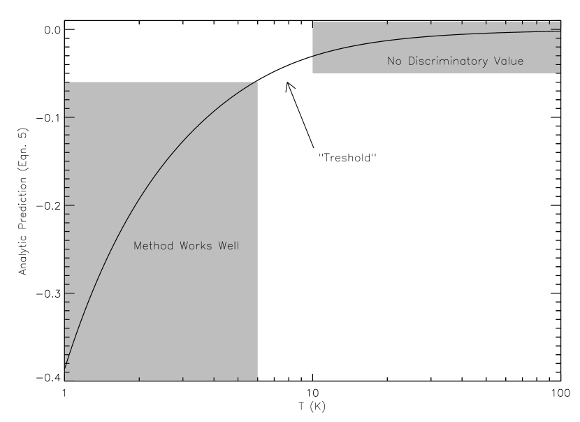
We next investigate the accuracy in estimating temperatures from observations at 3 wavelengths, using Equation (4). We first consider observations at 450, 850, and 1200 m, the three “popular” wavelengths used in the Schnee et al. (2007) study. Figure (9) shows the analytic prediction used to determine T from expression (4b) for temperatures between 1 - 100 K. At temperatures 7 - 10 K, the analytic prediction is very sensitive to the temperature. Thus, even though errors in the fluxes will produce an inaccurate value in expression (4a) for comparison with the analytic prediction of expression (4b), the derived temperature will still be close to the actual temperature of the emitting medium. At temperatures 7 - 10 K, however, the analytic prediction is not very sensitive to the temperature. Thus, even small errors in the flux, due to noise and/or other observational uncertainties, will result in grossly erroneous temperature estimates.
To investigate the effect of noise on the determination of temperature using equation 4, we have run a number of Monte-Carlo simulations. In these simulations, the emergent flux of a source at constant temperature (eqn. [1]) is modified by some chosen level of Gaussian noise, representing random errors in real observations. These “observed” fluxes at three wavelengths are used in expression (4a) to compare with the analytic prediction of expression (4b).
The uncertainties in the observations of Schnee et al. (2007) were estimated at 12%, 4%, and 10% for the 450, 850, and 1200 m observations, respectively. We use those uncertainties in our first simulated observations. We “observe” the extended source at 10,000 positions (or, equivalently, 10,000 times at a single location on the sky) at those three wavelengths. The flux ratios, using the noisy fluxes in expression (4a), from two sources at 10 K and 5 K are shown in Figure 10. The mean values of the flux ratio recovers the true temperature reasonably accurately. Also marked are the levels (as well as the levels for the 5 K source). At 10 K, even at the level, the flux ratio does not lie in the 1 - 100 K range of the analytic prediction shown in Figure 9. However, for the source at 5 K, at the level the derived temperature only differs from the true temperature by a factor of . At 10 K (and higher) temperatures, Figure 9 shows that the analytic prediction does not vary much with temperature, so any error in the flux ratio will correspond to a temperature that deviates significantly from the true temperature. For a 5 K source, the analytic prediction varies significantly with slight variations in temperature, so errors in the flux ratio will still produce reasonably accurate temperature estimates. This test has shown that with observations at 450, 850, and 1200 m, one can only be confident in the ratio method if the estimated temperatures are 5 K. For temperatures greater than the turn-over temperature in Figure 9 ( 7 - 10 K), the derived temperatures cannot be deemed accurate.
The temperature at which analytic prediction shifts from a strong temperature dependence to a weak temperature dependence is determined by the particular wavelengths used in expression (4b). In this sense, the ideal set of three wavelengths would shift the turn-over temperature to much higher values. In order to test the sensitivity of the turn-over temperature to the particular values of wavelengths, we have run a series of Monte-Carlo simulations as described above; we varied both the set of 3 wavelengths, as well as the (constant) temperature of the source.
In order to locate the turn-over temperature, we define a threshold temperature such that a range in the flux ratios corresponds to estimated temperatures that are within a factor of 2 of the actual source temperature . For example, consider a source at = 21 K observed at three given wavelengths. If the range of derived temperatures included in the level of the flux ratio includes temperatures 42 K, then we know that K for that set of wavelengths. If we then run another simulation on a source with = 20 K, with the same three wavelengths, and find that the maximum derived temperature in the 3 range is K, then we set K for this set of three wavelengths. Our definition of is arbitrary, and can of course be set to correspond to a higher accuracy temperature estimate; the goal here is simply to compare how well observations with varying wavelengths can reproduce source temperatures to a chosen level of accuracy. We note that at the -3 level, the difference of is always less than that difference at the +3 level, due to the logarithmic functional form of the analytic prediction; at lower flux ratios, corresponding to lower values of the analytic prediction (eqn. [4b]), the derived temperature is less sensitive to uncertainties in the fluxes (see Figs. 9 - 10).
Figure 11 shows the threshold temperatures, for given wavelength ratios and , where .444Table 3 in the Appendix explicitly lists the threshold temperatures for various sets of wavelengths, along with the wavelength ratios. Our choice of the three wavelengths span the range 70 - 3000 m. These particular wavelengths are shown because many of them are included in the wavebands of the upcoming Herschel and Planck missions. For simplicity, we assume a 10% noise level in the fluxes at all three wavelengths. A clear trend is immediately apparent in Figure 11. The highest values of occur when the two ratios and are simultaneously large. However, for a given ratio or there is a limit to how large the other ratio can be, beyond which decreases. From Table 3, the highest is achieved when m and m. At those wavelengths, both the Wien and R-J regimes of the SED for sources with 75 K are sampled.
Given two wavelengths that sample the Wien and R-J limits, the maximum temperature that can be reliably found is set by the middle wavelength : the maximum temperature is roughly that determined by Wien’s displacement law using as the wavelength corresponding to the flux peak. This general trend evidently dissolves as one or more of the boundary wavelengths or approaches . Since the wavelength corresponding to the SED peak is inversely proportional to the temperature, an increase of all three wavelengths by a constant factor would result in a decrease in by that same factor. Table 3 indeed shows such a trend. In short, the exact value of is dependent on all three wavelengths, as would be expected.
We have shown that given three wavelengths, one could determine a threshold temperature above which the ratio method will not be able to accurately derive the source temperature (to some chosen level of accuracy), due to uncertainties in the observations. In general, lower temperatures regions, such as cold, dense cores, can be more accurately measured through this method. In principle one could also determine which three wavelengths, and the associated uncertainties, are optimal to estimate a given temperature. However, such an analysis would not be as practical, since observers do not have an arbitrary choice as to what wavelengths they can observe, nor to any desired level of accuracy. After a brief discussion on estimating , we will show that fitting the SED directly to estimate the temperature is much more accurate than the ratio method, regardless of what three wavelengths are observed.
4.3 Estimating
In the ratio method, once a temperature estimate is obtained, it may be used in equation (5) to estimate . Only two fluxes are required in equation (5). For isothermal sources, any two fluxes will give good estimates of . Since the SED is more sensitive to noise at longer wavelengths, shorter wavelength fluxes will produce more accurate estimates. However, determining whether a source is isothermal itself is not trivial; as discussed in 3.4, with numerous fluxes this can be accomplished by systematically excluding short wavelength fluxes in a direct SED fit. When a source is not isothermal, the resulting temperature estimates from short wavelength fluxes will be highly inaccurate. The use of these incorrect temperatures in equation (5) will also produce incorrect estimates. Thus, an accurate estimate of is required before accurately estimating through equation (5).
Uncertainties in observations in the R-J tail will result in highly inaccurate estimates using the flux ratio method. For example, consider an isothermal source that is observed at three wavelengths, 450, 850, and 1200 µm. Fluxes that are inaccurate by a mere 3% can produce estimates that deviate from the actual value by 25%. For the simple 2 component source considered in 3.1.1 (and 4.1), and with flux uncertainties of only 5%, the estimated can be inaccurate by 50%. Thus, the flux ratio method gives highly uncertain estimates of .
5 Comparison of Fitting and Flux Ratio Methods involving Three Fluxes
In this section, using simulated observations of a dense core with temperature and density gradients, we compare the temperature estimate from direct SED fit to that derived from a flux ratio. Fluxes are only “observed” at three wavelengths, and include uncertainty due to noise, requiring that one of the three parameters in the fit (, , or ) is held fixed.
One approach to carry out the comparison would be to construct SEDs throughout the volume of the core, using equations (1)-(2), assuming a fixed value for . We could then integrate along all lines of sight to obtain the emergent intensity at three wavelengths, and then carry out the fitting, as we did in 3, or use the flux ratio method to estimate the temperature.
An alternative approach, which we choose to use here, is to utilize a radiative transfer (RT) code. With an RT simulation, the dust properties can be set using real dust optical constants. We thus use the radiative transfer code MOCASSIN (Ercolano et al., 2005). MOCASSIN is a 3D code that uses a Monte Carlo approach to the transfer of radiation through an arbitrary medium (Ercolano et al., 2003, 2008).
Our spherically symmetric model core emits radiation according to the emissivity properties of the dust. The physical properties of the core, such as the density and temperature profiles, as well as the dust properties, are held constant. Since we are only interested in the form the observed SED, and not the detailed distribution, the computational grid only has 16 16 16 zones, which follows the propagation of radiation through one-quarter of a spherical model core, with appropriate boundary conditions. The overall dimensions of the grid is 0.1 pc3; the resolution of an individual zone is comparable to the resolution of the TMC-1C maps presented by Schnee & Goodman (2005) and Schnee et al. (2007). As radiation (or energy packets) from all spatial locations traverses through the cloud, it is absorbed and re-emitted by the dust. However, we maintain the original temperature of the dust throughout the simulation. In this sense, the temperature of the core is set by some external source, such as an ambient interstellar radiation field, which is not explicitly included in our model. Radiation that emerges out of the core contributes to the “observed” flux. The emergent flux will thus be proportional to the density along the line of sight; the resulting observed 2D map of the core will scale with the 3D density integrated over the line of sight. We can then apply the flux ratio and fitting methods to estimate the temperature at each location on the 2D map.
We construct a core with a Bonnor-Ebert like density profile, where the density is constant in the central regions, but then drops off as the square of the radius. The temperature of this core is also constant in the central regions, but then increases logarithmically with radius. The temperature of the core varies from 7.5 K at the inner regions, to 12 K at the edge of the core. Such values span temperatures near the threshold temperature of the flux ratio method using 450, 850, and 1200 m fluxes, as well as temperatures well into the regime where the method becomes extremely sensitive to noise.
Figure 12 shows the core temperatures, both the actual temperature and the recovered ones. The ratio method produces a spread of temperatures at any given radius, due to noise introduced by the finite number of photons tracked in the simulation. A similar simulation of a core with constant density and constant temperature produces normally distributed fluxes with 10%. Despite the scatter in the observed fluxes, a general trend of decreasing temperature with decreasing radius is apparent. Towards the innermost regions, the flux ratio method overestimates the temperature more so than in the outer regions. This occurs because in the inner regions of the 2D observed map there is still a contribution to the flux from the warmer dust at larger radii, from matter lying above the colder central regions. At large radii, line of sight variations in temperature and density is minimized, so the mean of the flux ratio estimated temperatures corresponds well with the actual temperatures. Using the estimated temperatures from the flux ratio method in equation 5 gives . This is in good agreement with our choice of silicate grains in the simulation, which should have =2 (Draine & Lee, 1984).
In performing a fit to only three fluxes at each location, one of the free parameters must be held fixed. Since the flux ratio method produces a estimate that is well constrained, even though shows relatively higher levels of scatter, we hold fixed at that value. As shown in Figure 12, the temperatures obtained through such a fit are also overestimated at small radii. But, the scatter in the estimated temperatures is much smaller using a constrained SED fit (i.e. fixed) compared with the flux ratio method.
Also plotted on Figure 12 is the true column temperature (i.e. density weighted temperature). Each location (or grid zone) in the 2D map corresponds to a line of sight through the 3D core. We integrate the temperature along the line of sight at each location in the 2D map, weighted by the 3D densities used to construct the core. Evidently, the fit temperatures coincide remarkably well with the column temperature. The range in temperatures from the flux ratio method is also spread more evenly about the column temperature than the actual 3D temperature. At the innermost regions, there remains a slight offset. In general, though, the temperature estimates are certainly more representative of the “column temperature” than the true temperature of the core. This is not too surprising, because the observed flux indeed encodes information about all matter along a line of sight.
Had we assumed a different (and thus incorrect) value of that was held fixed in the fit, the best fit temperature would be systematically offset from the column temperature. For a 10 K isothermal source, fixing at 1.7 and 2.3 would produce fit temperatures of 12 and 9 K, respectively, using fluxes at 450, 850, and 1200 µm. The results of our simple tests suggest that though the flux ratio method can give highly uncertain temperature estimates from three fluxes, due to line of sight temperature variations, those temperatures can still provide a decent first estimate for the (mean) spectral index (as found by Schnee et al. (2007) for isothermal sources). This estimate for can then be held fixed in a fit which will recover temperatures with less scatter, and in close agreement with the column temperature.
6 Discussion
A flux ratio method to estimate the temperatures can also be constructed with four wavelengths. The form of the analytical prediction for four wavelengths is similar to expression (4b). We have also performed Monte Carlo simulations to test whether a flux ratio method using four wavelengths produces more accurate estimates of the source temperature, compared with a flux ratio method involving only three wavelengths. The general trends we found for three wavelengths remains: lower wavelength observations produce less scatter in the estimated temperatures, and that the fluxes should sample different regions of the spectrum to obtain decent temperature estimates. However, the maximum temperature at which the turn over occurs for any set of 4 wavelengths listed in Table 3 is 65 K, for our definition of in 4.2.
When fluxes at four wavelengths are available, however, a direct fit may be employed to estimate (and the absolute scaling ) along with the temperature. Since determining through the the flux ratio (eqn. [5]) could give contradictory estimates depending on which the fluxes are used, a direct SED fit is preferable. We did not find any advantage of using the flux ratio method to determine the temperature using four wavelengths compared with a direct fit of a modified blackbody SED.
In all of our tests, we have only considered sources with constant spectral indices. A line of sight may also have a variations in , and would further complicate the estimation of dust temperature. It may be reasonable to assume that the dust emissivity is constant within a core, where temperatures only vary by 10 K. But for lines of sight extending through a wider range in density and temperature, such as the lower density, warmer gas surrounding sites of recent star formation, assigning a single value for the spectral index may lead to errors in determining the temperature. A thorough investigation of spectral index variations over a range of environments would be required to quantify its effect on the emergent SED.
7 Summary
We have investigated the effect of noise and line of sight temperature variations on two common methods used to estimate the dust temperature and spectral index of cold star forming cores using continuum observations. One method is a direct fit to a modified blackbody spectrum. The second method involves the use of flux ratios.
We demonstrate that employing an isothermal modified blackbody equation (eqn. [1]-[2]) may lead to highly inaccurate dust temperature and spectral index estimates. Least squares SED fits to fluxes in the R-J regime, as opposed to the Wien regime, may provide accurate spectral index and density weighted temperature, or column temperature, estimates. For conditions typical of starless cores, fluxes in the R-J regime have wavelengths 600 µm. However, the fits to fluxes in the R-J regime are rather sensitive to observational uncertainties, such as noise.
The flux ratio method may also provide inaccurate parameter estimates due to line of sight temperature variations, and is also very sensitive to noise. In a comparison of the flux ratio and least squares fitting methods when only three fluxes are available, we find that a direct fit with the spectral index held fixed provides more accurate estimates of the column temperature. The flux ratio method can be initially used to estimate the value of the spectral index to be held fixed for a least-squares SED fit.
We summarize our main findings in more detail here:
1) Line of sight temperature variations can lead to inaccurate temperature and spectral index estimates when fitting a power-law-modified blackbody SED to observed fluxes. Near the SED peak of sources with temperature variations, the spectrum is poorly fit by an isothermal spectrum. For longer wavelength observations in the Rayleigh-Jeans regime of the spectrum, and with minimal observational uncertainties, a fit can accurately recover the spectral index (if it is constant), and provides a good estimate of the upper limit of the column temperature. However, at these long (Rayleigh-Jeans) wavelengths a fit is extremely sensitive to noise.
2) Short wavelength observations ( 600 µm) are still useful, for they can indicate whether an observed source contains temperature variations. For starless-core-like sources with temperature variations, the resulting fit decreases and fit increases when systematically excluding short wavelength fluxes from the fit. Published data of sources in Taurus and Orion by Stepnik et al. (2003) and Dupac et al. (2001), respectively, show these apparent trends, but an isothermal description with no systematic variations in still cannot be strictly ruled out, due to the uncertainties. Observed fluxes by Kirk et al. (2007) of B68, though, produce lower fit temperatures and higher fit spectral indices when short wavelength fluxes are omitted, strongly suggestive of dust temperature variations along the line-of-sight. We estimate an upper limit of 10.8 0.1 K for the temperature of the coldest region within B68; and if the spectral index is constant throughout the core, then we estimate 2.4.
3) SED fits to fluxes in the Rayleigh-Jeans regime are very sensitive to noise, even for isothermal sources. The fits may produce a spurious inverse - relationship, similar to the trend discussed by Dupac et al. (2003). SED fits may be more accurate when fluxes with wavelengths that span the SED peak are available, compared with fits to fluxes solely in the Rayleigh-Jeans regime. However, fits to fluxes near the SED peak would be inaccurate if the source contains line of sight temperature variations. In general, for objects that are cool pockets in higher density regions, such as starless cores, SED fits that produce higher temperatures also (artificially) give lower spectral indices.
4) We find that, due to noise uncertainties in any observation, the flux ratio method is most accurate for emission originating from cold isothermal regions. For a source with a constant temperature, there may be a range in the estimated temperature, due to the uncertainties in the observations. At low temperatures, this spread is small; at higher temperatures the spread can be rather large, rendering the temperature estimate highly inaccurate. The precise temperature, or threshold temperature, for which the method shifts from relatively accurate to inaccurate is dependent on the observed wavelengths (as well as the desired level of accuracy, see Fig. 11 and Table 3). For example, for fluxes at 450, 850, and 1200 µm, the flux ratio method can provide accurate temperature estimates only for sources with 7 - 10 K (Fig. 9).
5) Using Monte Carlo simulations, we quantified the dependence of the turn over temperature on the set of observed wavelengths. Ideally, as one might intuitively expect, two of the three wavelengths should sample the Wien and the Rayleigh-Jeans regime of the SED, with the final wavelength lying at intermediate values. Further, a greater separation between the wavelengths results in more accurate temperature estimates. In general, higher temperatures can be more accurately measured when the observations include short wavelength far-infrared observations 100 m; at short wavelengths, however, there may be a contribution from stars and transiently heated very small grains to the observed flux.
6) A reasonably accurate estimate of can be obtained from the mean of the estimates derived from the flux ratio method involving three fluxes. For fluxes at 450, 850, and 1200 µm, with 10% uncertainties, can be estimated to within 5% of the true source value. This value can then be held fixed in a constrained SED fit to the three fluxes to estimate the temperature with less scatter than an estimate from the flux ratio method (Fig. 12). With four or more observations may be one of the free parameters in the fit (and, of course, the fit is better constrained).
7) The temperatures estimated through the SED fit and ratio methods, however, cannot be used to assign the absolute temperature to a given 3D location in a cold core. The projected SED contains information from all emitting matter along any line of sight. The measured temperature is more representative of the column temperature. In this regard, the estimated temperatures provide an upper limit for the coldest temperature along the line of sight.
Appendix A Appendix
References
- Adams et al. (1987) Adams, F. C., Lada, C. J., & Shu, F. H. 1987, ApJ, 312, 788
- Alves et al. (2001) Alves, J. F., Lada, C. J., & Lada, E. A. 2001, Nature, 409, 159
- Andre et al. (1993) Andre, P., Ward-Thompson, D., & Barsony, M. 1993, ApJ, 406, 122
- Bacmann et al. (2000) Bacmann, A., André, P., Puget, J.-L., Abergel, A., Bontemps, S., & Ward-Thompson, D. 2000, A&A, 361, 555
- Benson & Myers (1989) Benson, P. J. & Myers, P. C. 1989, ApJS, 71, 89
- Bergin et al. (2002) Bergin, E. A., Alves, J., Huard, T., & Lada, C. J. 2002, ApJ, 570, L101
- Bonnor (1956) Bonnor, W. B. 1956, MNRAS, 116, 351
- Crapsi et al. (2007) Crapsi, A., Caselli, P., Walmsley, M. C., & Tafalla, M. 2007, A&A, 470, 221
- Doty & Leung (1994) Doty, S. D. & Leung, C. M. 1994, ApJ, 424, 729
- Doty & Palotti (2002) Doty, S. D. & Palotti, M. L. 2002, MNRAS, 335, 993
- Draine & Lee (1984) Draine, B. T. & Lee, H. M. 1984, ApJ, 285, 89
- Dupac et al. (2003) Dupac, X., Bernard, J.-P., Boudet, N., Giard, M., Lamarre, J.-M., Mény, C., Pajot, F., Ristorcelli, I., Serra, G., Stepnik, B., & Torre, J.-P. 2003, A&A, 404, L11
- Dupac et al. (2002) Dupac, X., Giard, M., Bernard, J.-P., Boudet, N., Lamarre, J.-M., Mény, C., Pajot, F., Pointecouteau, É., Ristorcelli, I., Serra, G., Stepnik, B., & Torre, J.-P. 2002, A&A, 392, 691
- Dupac et al. (2001) Dupac, X., Giard, M., Bernard, J.-P., Lamarre, J.-M., Mény, C., Pajot, F., Ristorcelli, I., Serra, G., & Torre, J.-P. 2001, ApJ, 553, 604
- Ebert (1955) Ebert, R. 1955, Zeitschrift fur Astrophysik, 37, 217
- Ercolano et al. (2005) Ercolano, B., Barlow, M. J., & Storey, P. J. 2005, MNRAS, 362, 1038
- Ercolano et al. (2003) Ercolano, B., Barlow, M. J., Storey, P. J., & Liu, X.-W. 2003, MNRAS, 340, 1136
- Ercolano et al. (2008) Ercolano, B., Young, P. R., Drake, J. J., & Raymond, J. C. 2008, ApJS, 175, 534
- Evans et al. (2001) Evans, II, N. J., Rawlings, J. M. C., Shirley, Y. L., & Mundy, L. G. 2001, ApJ, 557, 193
- Foster & Goodman (2006) Foster, J. B. & Goodman, A. A. 2006, ApJ, 636, L105
- Goldsmith (2001) Goldsmith, P. F. 2001, ApJ, 557, 736
- Hildebrand (1983) Hildebrand, R. H. 1983, QJRAS, 24, 267
- Kauffmann et al. (2008) Kauffmann, J., Bertoldi, F., Bourke, T. L., Evans, II, N. J., & Lee, C. W. 2008, A&A, 487, 993
- Keene et al. (1980) Keene, J., Hildebrand, R. H., Whitcomb, S. E., & Harper, D. A. 1980, ApJ, 240, L43
- Kirk et al. (2007) Kirk, J. M., Ward-Thompson, D., & André, P. 2007, MNRAS, 375, 843
- Kramer et al. (2003) Kramer, C., Richer, J., Mookerjea, B., Alves, J., & Lada, C. 2003, A&A, 399, 1073
- Kuan et al. (1996) Kuan, Y.-J., Mehringer, D. M., & Snyder, L. E. 1996, ApJ, 459, 619
- Lada (1987) Lada, C. J. 1987, in IAU Symposium, Vol. 115, Star Forming Regions, ed. M. Peimbert & J. Jugaku, 1–17
- Lada et al. (1994) Lada, C. J., Lada, E. A., Clemens, D. P., & Bally, J. 1994, ApJ, 429, 694
- Leung (1975) Leung, C. M. 1975, ApJ, 199, 340
- Li & Draine (2001) Li, A. & Draine, B. T. 2001, ApJ, 554, 778
- Mathis (1990) Mathis, J. S. 1990, ARA&A, 28, 37
- Oldham et al. (1994) Oldham, P. G., Griffin, M. J., Richardson, K. J., & Sandell, G. 1994, A&A, 284, 559
- Schlegel et al. (1998) Schlegel, D. J., Finkbeiner, D. P., & Davis, M. 1998, ApJ, 500, 525
- Schnee et al. (2006) Schnee, S., Bethell, T., & Goodman, A. 2006, ApJ, 640, L47
- Schnee & Goodman (2005) Schnee, S. & Goodman, A. 2005, ApJ, 624, 254
- Schnee et al. (2007) Schnee, S., Kauffmann, J., Goodman, A., & Bertoldi, F. 2007, ApJ, 657, 838
- Schnee et al. (2005) Schnee, S. L., Ridge, N. A., Goodman, A. A., & Li, J. G. 2005, ApJ, 634, 442
- Shetty et al. (2009) Shetty, R., Kauffmann, J., Schnee, S., Goodman, A. A., & Ercolano, B. 2009, ApJ Accepted, astro-ph/0902.0636
- Stepnik et al. (2003) Stepnik, B., Abergel, A., Bernard, J.-P., Boulanger, F., Cambrésy, L., Giard, M., Jones, A. P., Lagache, G., Lamarre, J.-M., Meny, C., Pajot, F., Le Peintre, F., Ristorcelli, I., Serra, G., & Torre, J.-P. 2003, A&A, 398, 551
- Teuben (1995) Teuben, P. 1995, in ASP Conf. Ser. 77: Astronomical Data Analysis Software and Systems IV, ed. R. A. Shaw, H. E. Payne, & J. J. E. Hayes, 398–+
- Ward-Thompson et al. (2002) Ward-Thompson, D., André, P., & Kirk, J. M. 2002, MNRAS, 329, 257
- Zucconi et al. (2001) Zucconi, A., Walmsley, C. M., & Galli, D. 2001, A&A, 376, 650
| Scenario | 3.1 | 3.2 | 3.3 | 3.4 | 4.1 | 4.2 | 4.3 | 5 | 6 |
|---|---|---|---|---|---|---|---|---|---|
| Least Squares Fitting | ✓ | ✓ | ✓ | AppaaApplication: SED fits to fluxes from published observations | ✓ | ||||
| Flux Ratio Method | ✓ | ✓ | ✓ | ✓ | |||||
| constant | ✓ | ✓ | ✓ | ||||||
| Two Medium | ✓ | ✓ | ✓ | ||||||
| Gradient in | ✓ | ✓ | |||||||
| constant | ✓ | ✓ | ✓ | AppaaApplication: SED fits to fluxes from published observations | FixedbbChoice of required in method | N/Acc is not required or recovered from method | Deriveddd can derived from flux ratio method involving 2 fluxes | ✓ | |
| variable | ✓ | ||||||||
| Two Fluxes | ✓ | ||||||||
| Three Fluxes | ✓ | ✓ | |||||||
| Fluxes 3 | ✓ | AppaaApplication: SED fits to fluxes from published observations | ✓ | ||||||
| Fluxes 3 | ✓ | ✓ | |||||||
| Without Noise | ✓ | ✓ | ✓ | ||||||
| With Noise | ✓ | AppaaApplication: SED fits to fluxes from published observations | ✓ | ✓ | ✓ |
| Observed , | Assumed aaModel Spectral index = 2.0 | Source | Derived | |
|---|---|---|---|---|
| (µm) | (%) | (K) | (K) | |
| Isothermal: | ||||
| 450,850 | 1.9 | 0 | 10 | 10.5 |
| 450,850 | 2.0 | 0 | 10 | 10.0 |
| 450,850 | 2.1 | 0 | 10 | 9.5 |
| 450,850 | 1.9 | 10 | 10 | 10.6 1.3 |
| 450,850 | 2.0 | 10 | 10 | 10.0 1.2 |
| 450,850 | 2.1 | 10 | 10 | 9.6 1.0 |
| 1200,2100 | 1.9 | 0 | 10 | 12.1 |
| 1200,2100 | 2.0 | 0 | 10 | 10.0 |
| 1200,2100 | 2.1 | 0 | 10 | 8.6 |
| 1200,2100 | 1.9 | 10 | 10 | 14.5 12.6 |
| 1200,2100 | 2.0 | 10 | 10 | 12.1 9.4 |
| 1200,2100 | 2.1 | 10 | 10 | 10.2 7.0 |
| 2-Component Source (2COMPd): | ||||
| 450,850 | 1.9 | 0 | 10.9 | 12.5 |
| 450,850 | 2.0 | 0 | 10.9 | 11.7 |
| 450,850 | 2.1 | 0 | 10.9 | 11.0 |
| 450,850 | 1.9 | 10 | 10.9 | 12.7 2.0 |
| 450,850 | 2.0 | 10 | 10.9 | 11.8 1.7 |
| 450,850 | 2.1 | 10 | 10.9 | 11.1 1.5 |
| 1200,2100 | 1.9 | 0 | 10.9 | 13.8 |
| 1200,2100 | 2.0 | 0 | 10.9 | 11.1 |
| 1200,2100 | 2.1 | 0 | 10.9 | 9.3 |
| 1200,2100 | 1.9 | 10 | 10.9 | 15.4 13.4 |
| 1200,2100 | 2.0 | 10 | 10.9 | 13.5 10.9 |
| 1200,2100 | 2.1 | 10 | 10.9 | 11.3 8.2 |
| aa chosen as the temperature at which is within a factor of 2 of the source temperature. | |||||
|---|---|---|---|---|---|
| 70 | 110 | 170 | 1.55 | 1.57 | 18 |
| 70 | 110 | 350 | 3.18 | 1.57 | 38 |
| 70 | 110 | 450 | 4.09 | 1.57 | 41 |
| 70 | 110 | 850 | 7.73 | 1.57 | 47 |
| 70 | 110 | 1200 | 10.91 | 1.57 | 49 |
| 70 | 110 | 1380 | 12.55 | 1.57 | 50 |
| 70 | 110 | 2100 | 19.09 | 1.57 | 51 |
| 70 | 110 | 3000 | 27.27 | 1.57 | 52 |
| 70 | 170 | 350 | 2.06 | 2.43 | 39 |
| 70 | 170 | 450 | 2.65 | 2.43 | 47 |
| 70 | 170 | 850 | 5.00 | 2.43 | 55 |
| 70 | 170 | 1200 | 7.06 | 2.43 | 57 |
| 70 | 170 | 1380 | 8.12 | 2.43 | 58 |
| 70 | 170 | 2100 | 12.35 | 2.43 | 59 |
| 70 | 170 | 3000 | 17.65 | 2.43 | 60 |
| 70 | 350 | 450 | 1.29 | 5.00 | 18 |
| 70 | 350 | 850 | 2.43 | 5.00 | 47 |
| 70 | 350 | 1200 | 3.43 | 5.00 | 54 |
| 70 | 350 | 1380 | 3.94 | 5.00 | 55 |
| 70 | 350 | 2100 | 6.00 | 5.00 | 59 |
| 70 | 350 | 3000 | 8.57 | 5.00 | 61 |
| 70 | 450 | 850 | 1.89 | 6.43 | 37 |
| 70 | 450 | 1200 | 2.67 | 6.43 | 50 |
| 70 | 450 | 1380 | 3.07 | 6.43 | 52 |
| 70 | 450 | 2100 | 4.67 | 6.43 | 57 |
| 70 | 450 | 3000 | 6.67 | 6.43 | 60 |
| 70 | 850 | 1200 | 1.41 | 12.14 | 22 |
| 70 | 850 | 1380 | 1.62 | 12.14 | 28 |
| 70 | 850 | 2100 | 2.47 | 12.14 | 44 |
| 70 | 850 | 3000 | 3.53 | 12.14 | 52 |
| 70 | 1200 | 1380 | 1.15 | 17.14 | 9 |
| 70 | 1200 | 2100 | 1.75 | 17.14 | 29 |
| 70 | 1200 | 3000 | 2.50 | 17.14 | 42 |
| 70 | 1380 | 2100 | 1.52 | 19.71 | 23 |
| 70 | 1380 | 3000 | 2.17 | 19.71 | 37 |
| 70 | 2100 | 3000 | 1.43 | 30.00 | 19 |
| 110 | 170 | 350 | 2.06 | 1.55 | 18 |
| 110 | 170 | 450 | 2.65 | 1.55 | 21 |
| 110 | 170 | 850 | 5.00 | 1.55 | 27 |
| 110 | 170 | 1200 | 7.06 | 1.55 | 29 |
| 110 | 170 | 1380 | 8.12 | 1.55 | 30 |
| 110 | 170 | 2100 | 12.35 | 1.55 | 31 |
| 110 | 170 | 3000 | 17.65 | 1.55 | 33 |
| 110 | 350 | 450 | 1.29 | 3.18 | 11 |
| 110 | 350 | 850 | 2.43 | 3.18 | 30 |
| 110 | 350 | 1200 | 3.43 | 3.18 | 36 |
| 110 | 350 | 1380 | 3.94 | 3.18 | 37 |
| 110 | 350 | 2100 | 6.00 | 3.18 | 42 |
| 110 | 350 | 3000 | 8.57 | 3.18 | 45 |
| 110 | 450 | 850 | 1.89 | 4.09 | 24 |
| 110 | 450 | 1200 | 2.67 | 4.09 | 32 |
| 110 | 450 | 1380 | 3.07 | 4.09 | 34 |
| 110 | 450 | 2100 | 4.67 | 4.09 | 41 |
| 110 | 450 | 3000 | 6.67 | 4.09 | 44 |
| 110 | 850 | 1200 | 1.41 | 7.73 | 14 |
| 110 | 850 | 1380 | 1.62 | 7.73 | 19 |
| 110 | 850 | 2100 | 2.47 | 7.73 | 29 |
| 110 | 850 | 3000 | 3.53 | 7.73 | 36 |
| 110 | 1200 | 1380 | 1.15 | 10.91 | 6 |
| 110 | 1200 | 2100 | 1.75 | 10.91 | 20 |
| 110 | 1200 | 3000 | 2.50 | 10.91 | 29 |
| 110 | 1380 | 2100 | 1.52 | 12.55 | 15 |
| 110 | 1380 | 3000 | 2.17 | 12.55 | 25 |
| 110 | 2100 | 3000 | 1.43 | 19.09 | 13 |
| 170 | 350 | 450 | 1.29 | 2.06 | 6 |
| 170 | 350 | 850 | 2.43 | 2.06 | 17 |
| 170 | 350 | 1200 | 3.43 | 2.06 | 20 |
| 170 | 350 | 1380 | 3.94 | 2.06 | 21 |
| 170 | 350 | 2100 | 6.00 | 2.06 | 23 |
| 170 | 350 | 3000 | 8.57 | 2.06 | 25 |
| 170 | 450 | 850 | 1.89 | 2.65 | 15 |
| 170 | 450 | 1200 | 2.67 | 2.65 | 19 |
| 170 | 450 | 1380 | 3.07 | 2.65 | 21 |
| 170 | 450 | 2100 | 4.67 | 2.65 | 24 |
| 170 | 450 | 3000 | 6.67 | 2.65 | 27 |
| 170 | 850 | 1200 | 1.41 | 5.00 | 10 |
| 170 | 850 | 1380 | 1.62 | 5.00 | 12 |
| 170 | 850 | 2100 | 2.47 | 5.00 | 19 |
| 170 | 850 | 3000 | 3.53 | 5.00 | 24 |
| 170 | 1200 | 2100 | 1.75 | 7.06 | 14 |
| 170 | 1200 | 3000 | 2.50 | 7.06 | 19 |
| 170 | 1380 | 2100 | 1.52 | 8.12 | 11 |
| 170 | 1380 | 3000 | 2.17 | 8.12 | 17 |
| 170 | 2100 | 3000 | 1.43 | 12.35 | 9 |
| 350 | 450 | 2100 | 4.67 | 1.29 | 5 |
| 350 | 450 | 3000 | 6.67 | 1.29 | 6 |
| 350 | 850 | 1380 | 1.62 | 2.43 | 6 |
| 350 | 850 | 2100 | 2.47 | 2.43 | 9 |
| 350 | 850 | 3000 | 3.53 | 2.43 | 10 |
| 350 | 1380 | 3000 | 2.17 | 3.94 | 8 |