Spins coupled to a Spin Bath: From Integrability to Chaos

Abstract

Motivated by the hyperfine interaction of electron spins with surrounding nuclei, we investigate systems of central spins coupled to a bath of noninteracting spins in the framework of random matrix theory. With increasing number of central spins a transition from Poissonian statistics to the Gaussian orthogonal ensemble occurs which can be described by a generalized Brody distribution. These observations are unaltered upon applying an external magnetic field. In the transition region, the classical counterparts of the models studied have mixed phase space.

Spins coupled to a bath of other spin degrees of freedom occur in a variety of nanostructures including semiconductor quantum dots Petta05 ; Koppens06 ; Hanson07 ; Braun05 , carbon nanotube quantum dots Churchill08 , phosphorus donors in silicon Abe04 , nitrogen vacency centers in diamond Jelezko04 ; Childress06 ; Hanson08 , and molecular magnets Ardavan07 . A large portion of the presently very high both experimental and theoretical interest in such systems is due to proposals to utilize such structures for quantum information processing Loss98 ; Kane98 ; Leuenberger01 . Here the central spins play the role of the qubit whereas the surrounding bath spins act as an decohering environment. In the present letter we investigate very basic properties of such so-called central spin systems in terms of spectral statistics and random matrix theory Guhr98 .

The generic Hamiltonian is given by

$${\cal H}=\sum_{\alpha=1}^{N_{c}}\vec{S}_{\alpha}\cdot\sum_{i=1}^{N}A_{i}^{(\alpha)}\vec{I}_{i}$$ (1)

describing $N_{c}$ central spins $\vec{S}_{\alpha}$ coupled to $N$ bath spins $\vec{I}_{i}$, typically $N\gg N_{c}$. Here we take all spins to be dimensionless quantum variables such that the coupling constants $A_{i}^{(\alpha)}$ have dimension of energy. A paradigmatic example is given by, say, a single spin of a conduction-band electron residing in a semiconductor quantum dot and being coupled via hyperfine contact interaction to the bath of surrounding nuclear spins. In a very typical material like gallium arsenide all nuclei have a spin of $I=3/2$ whereas in other systems like indium arsenide even spins of length $I=9/2$ occur. In fact, this hyperfine interaction with surrounding nuclei has been identified to be the limiting factor regarding coherent dynamics of electron spin qubits Petta05 ; Koppens06 ; Hanson07 ; Khaetskii02 . In the above example the hyperfine coupling constants $A_{i}^{(\alpha)}$ are proportional to the square modulus of the electronic wave function at the location of the nucleus and can therefore vary widely in magnitude. For the purposes of our statistical analysis here we shall take an even more radical point of view and choose the $A_{i}^{(\alpha)}$ at random. To be specific, we will choose the $A_{i}^{(\alpha)}$ from a uniform distribution within the interval $[0,1]$ and normalize them afterwards according to $\sum_{i}A_{i}^{(\alpha)}=1$ for each central spin. The data to be presented below is obtained by averaging over typically 500 random realizations of coupling parameters. Note that the Hamiltonian matrix represented in the usual basis of tensor-product eigentstates of $S_{\alpha}^{z}$, $I_{i}^{z}$ is always real and symmetric. Therefore, the natural candidate for a random matrix description of such systems is the Gaussian orthogonal ensemble (GOE) Guhr98 .

In the important case of a single central spin, $N_{c}=1$, the above model has the strong mathematical property of being integrable Gaudin76 ; Bortz07 . Moreover, this integrability is particularly robust as it is independent of the choice of the coupling parameters $A_{i}^{(1)}$ and the length of the spins which can even be chosen individually Gaudin76 ; Bortz07 . In fact, the model (1) for a single central spin has been the basis of numerous theoretical studies on decoherence properties of quantum dot spin qubits; see, for example, Refs. Khaetskii02 ; Merkulov02 ; Schliemann02 ; Coish08 ; Cywinski09 , for reviews also Schliemann03 ; Zhang07 ; Klauser07 . It is an interesting question, both from a practical as well as from an abstract point of view, to what extend the results of these investigations are linked to the integrability of the underlying idealized model. In particular, what changes may occur if the Hamiltonian deviates from the above simple case $N_{c}=1$ by, e.g., involving more than one central spin? Previous investigations of decoherence properties, making strongly restrictive assumptions on the coupling constants, predicted a significant dependence on whether the number of central spins is even or odd Dobrovitski03 ; Melikidze04 . In the following we will investigate Hamiltonians of the general type (1) within the framework of level statistics, i.e. generic spectral characteristics Guhr98 . For other studies of interacting quantum many-body systems using this method see e.g. Refs. Montambaux93 ; Georgeot98 ; Avishai02 .

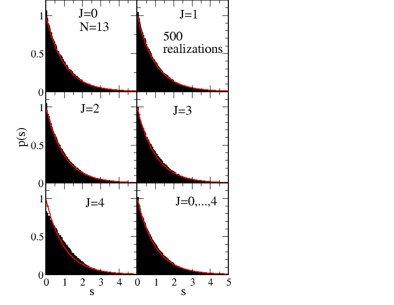
Figure 1: (Color online) Nearest-neighbor level spacing for a system of a single central spin $S_{1}=1/2$ and 13 bath spins of length $I=1/2$. The red curve is the exponential $p(s)=e^{-s}$.

The spectra generated numerically from the Hamiltonian (1) clearly have a nontrivial overall structure, i.e. the locally averaged density of states is not constant as a function of energy Schliemann02 ; Schliemann03 . Therefore an unfolding of these spectra has to be performed which results in a transformation onto a new spectral variable $s$ such that the mean level density is equal to unity Guhr98 . We have compared several standard numerical unfolding procedures and made sure that they yield consistent results. Fig. 1 shows the probability distribution $p(s)$ for the nearest-neighbor level spacing for a system of a single central spin $S_{1}=1/2$ and 13 bath spins of length $I=1/2$ for several subspaces of the total angular momentum $\vec{J}=\vec{S}_{1}+\sum_{i}\vec{I}_{i}$ where each multiplet is counted as a single enery level. The subspaces of highest $J=5,6,7$ have been discarded, and in the bottom right panel all probability distributions are joined. As to be expected for an integrable model, the level statistics follow a Poisson distribution resulting in an exponential level spacing distribution $p(s)=e^{-s}$. This is in contrast to the case of two central spins $S_{1}=S_{2}=1/2$ shown in Fig. 2. Here level repulsion takes clearly place, $p(0)=0$, although the data considerably deviates from the Wigner surmise for the GOE Guhr98 , $p(s)=(\pi/2)s\exp(-(\pi/4)s^{2})$.

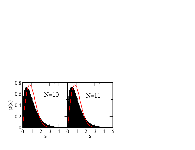
Figure 3: (Color online) The same data as in the bottom right panel of Fig. 2 but for $N=10$ and $N=11$ bath spins.

Obviously, our numerical studies are technically restricted to rather small system sizes, $N_{c}+N\leq 14$. This limitation, however, does not affect our results for the level statistics as demonstrated in Fig. 3 where we have plotted the same data as in the bottom right panel of Fig. 2 but for $N=10$ and $N=11$ bath spins. This insensitivity to the system size seen in the figure is a natural consequence of the unfolding of the spectra.

Fig 4 shows the joint level spacing distribution for $J=0,\dots,4$ and increasing number of central spins, where $p(s)$ approaches closer and closer the Wigner surmise. To quantify this observation we use the ansatz

$$p(s)=Bs^{\beta}e^{-As^{\alpha}}$$ (2)

with

$$B = \alpha(\Gamma((\beta+2)/\alpha))^{\beta+1}/(\Gamma((\beta+1)/\alpha))^{\beta+2}\,,$$ (3)

$$A = \left(\Gamma((\beta+2)/\alpha)/\Gamma((\beta+1)/\alpha)\right)^{\alpha}$$ (4)

such that $\int p(s)=\int sp(s)=1$. Clearly, $\alpha=1$, $\beta=0$ corresponds to an exponential distribution whereas $\alpha=2$, $\beta=1$ reporduces the Wigner surmise. The above ansatz generalizes the Brody distribution given by $\alpha=\beta+1$ Brody73 ; Guhr98 . As seen in Fig. 4, the numerical data is very well described by the above distribution, and for the case of $5$ central spins the Wigner surmise of the GOE is almost reached. In particular, our level statistics do not show any odd/even-effects with respect to the number of central spins as predicted in Refs. Dobrovitski03 ; Melikidze04 . We attribute this difference to the strongly restrictive assumptions made there giving rise to additional symmetries.

Moreover, in the case of two central spins it is instructive to rewrite the Hamiltonian in the following form,

$${\cal H} = (\vec{S}_{1}+\vec{S}_{2})\cdot\sum_{i}\frac{1}{2}(A_{i}^{(1)}+A_{i}^{(2)})\vec{I}_{i}$$ (5)

$$+ (\vec{S}_{1}-\vec{S}_{2})\cdot\sum_{i}\frac{1}{2}(A_{i}^{(1)}-A_{i}^{(2)})\vec{I}_{i}\,.$$

The two central spins $\vec{S}=\vec{S}_{1}+\vec{S}_{2}$ can couple to $S=0,1$. Since the coupling to the singlet $S=0$ vanishes, the first line in Eq. (5) is just the integrable Hamiltonian of a single central spin $S=1$, whereas the second line can be viewed as a perturbation. This term vanishes if the coupling constants are still random but chosen to be the same for each spin, $A_{i}^{(1)}=A_{i}^{(2)}$, resulting in an integrable model of two central spins, a prediction we have explicitly verified in our numerics; the latter model was also studied numerically in Ref. Dobrovitski03 .

The models studied so far have a common spin bath, i.e. each bath spin couples without any further restriction to each central spin. Regarding the generic example of two neighboring quantum dot spin qubits this is not particularly realistic since in this geometry one can obviously identify groups of nuclear spins which couple strongly to one of the electron spins but weakly to the other. The extreme case is given by two separate spin baths where the central spins can be coupled via an exchange interaction Burkard99 ; Schliemann01 , ${\cal H}^{\prime}={\cal H}+J_{ex}\vec{S}_{1}\cdot\vec{S}_{2}$. Here we find numerically that even arbitrary small exchange parameters $J_{ex}$ break integrability and lead to level repulsion. The corresponding level spacing distributions, however, are less accurately described by the ansatz (2). On the other hand, for large $|J_{ex}|$ the system approaches the integrable scenario since then the singlet and triplet subspace of the central spins are energetically more and more separated.

Let us now discuss the influence of an external magnetic field coupling to the central spins. In the case $N_{c}=1$ the resulting model is known to be integrable Gaudin76 ; Bortz07 , and also for $N_{c}>1$ the Hamiltonian can still be represented as a real and symmetric matrix. Indeed, we have not seen any qualitative difference in the level spacing distribution with and without an external magnetic field. In particular, we have not found any sign for a transition between the Gaussian orthogonal to the unitary ensemble (as appropriate for systems lacking time reversal symmetry Guhr98 ). In this sense, the application of an external magnetic field can be viewed as a “false symmetry breaking” which still preserves a “non-conventional time-reversal invariance” Avishai02 ; Haake00 . We note that recent theoretical works predict different time dependencies of spin dynamics in different magnetic-field regimes Coish08 ; Cywinski09 . These observations are not reflected by the level statistics. Thus, decoherence and the occurrence of integrability or chaoticity are independent phenomena in such systems, at least as far as the role of magnetic fields is concerned.

The data presented so far was obtained for bath spins of length $I=1/2$. Motivated by the large nuclear spins in semiconductor materials, we have also performed simulations for $I=1$ which also do not show any qualitative difference to the previous case. This is indeed to be expected since a spin bath of $I=1$ can be obtained from a bath with $I=1/2$ and twice the number of bath spins by grouping the spins into pairs and chosing the coupling parameters to be the same in each pair. Similar considerations apply to higher bath spins.

Let us come back to the case of two central spins. As seen in Figs. 2,4, this system appears to lie in between the integrable case and the predictions of random matrix theory. Thus, in the light of the Bohigas-Giannoni-Schmitt conjecture Bohigas84 , it is natural to speculate that the classical counterpart of this system has a mixed phase space consisting of areas of regular and of chaotic dynamics. The classical limit of a quantum spin system is naturally obtained via spin-coherent states, and a pair of classical canonically conjugate variables $p$, $q$ for each spin is given by $p=\cos\vartheta$, $q=\varphi$, where $\vartheta$, $\varphi$ are the usual angular coordinates of the classical spin unit vector Schliemann98 . We have performed numerical Runge-Kutta simulations of such classical dynamics for $N_{c}=2$ where one can easily treat systems of several thousand bath spins. However, to avoid the complications of such a high-dimensional phase space let us concentrate on the smallest nontrivial case of just two bath spins. Here we find indeed a close vicinity of regular and chaotic dynamics. An example is shown in Fig. 5 where we have plotted in the top panel a cut through the plane $I^{z}_{1}=I^{z}_{2}=0$ as a function of $p=S^{z}_{1}$, $q=\tan^{-1}(S^{y}_{1}/S^{x}_{1})$. The coupling constants are given by $A_{1}^{(1)}=1-A_{2}^{(1)}=0.75$, $A_{1}^{(2)}=1-A_{2}^{(2)}=0.52$, and the initial condition is $\vec{S}_{1}=-\vec{S}_{2}=(0,0,-1)$, $\vec{I}_{1}=(1,0,0)$, $\vec{I}_{2}=(0,1,0)$. This arrangement leads obviously to very regular dynamics, in stark contrast with the bottom panel where we have used the same initial condition but introduced a minute change in one pair of coupling constants, $A_{1}^{(2)}=1-A_{2}^{(2)}=0.5195$, resulting in a clearly chaotic orbit with an inhomogeneous phase space filling. Note that the observation that certain phase space curves are overlaid in the figure is due to the fact that the remaining six phase space variables are not uniquely determined by the condition $I^{z}_{1}=I^{z}_{2}=0$ and the conserved quantities ${\cal H}=0$, $\vec{J}=(1,1,0)$ but occur in several branches.

In summary, we have investigated central spin models via nearest-neighbor level spacing distributions. As the number of central spins increases a transition from Poissonian statistics to the Gaussian orthogonal ensemble sets in which can be described by a generalized Brody distribution. These observations are not affected by the finite system size in our numerical simulations and are unaltered upon applying an external magnetic field. In the transition region, the classical counterparts of the models studied have mixed phase space.

I thank M. Brack, K. Richter, S. Schierenberg, and T. Wettig for useful discussions. This work was supported by DFG via SFB 631.

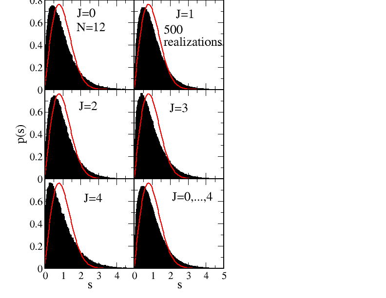
Figure 2: (Color online) Nearest-neighbor level spacing for a system of a two central spins $S_{1}=S_{2}=1/2$ and 12 bath spins of length $I=1/2$. The red curve is the GOE Wigner surmise.

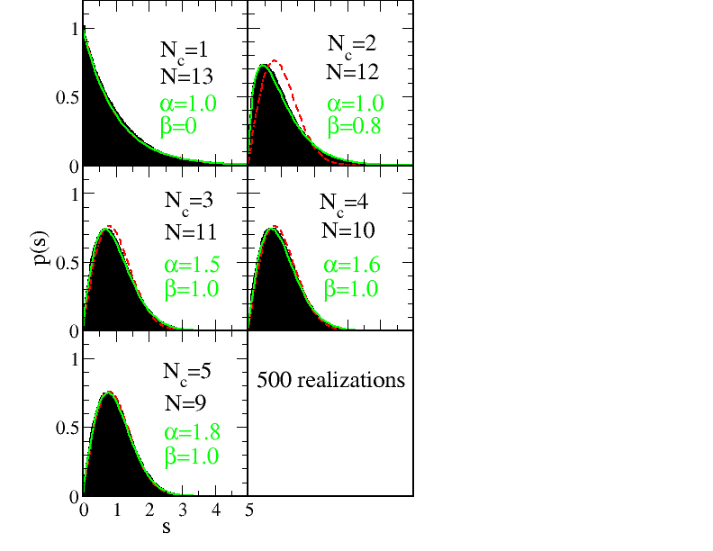
Figure 4: (Color online) Joint level spacing distribution for $J=0,\dots,4$ and increasing number of central spins. The red dashed lines are the exponential function ($N_{c}=1$) and the Wigner surmise ($N_{c}>1$). The green solid lines are a fit to the generalized Brody distribution (2).

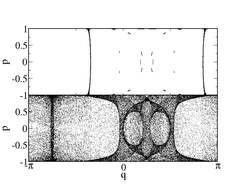
Figure 5: A cut through the plane $I^{z}_{1}=I^{z}_{2}=0$ of two different phase space orbits demonstrating the close vicinity of regular and chaotic dynamics in a system of two central spins (see text).

References

- (1) J. R. Petta et al., Science 309, 2180 (2005).
- (2) F. H. L. Koppens et al., Nature 442, 766 (2006).
- (3) R. Hanson et al., Rev. Mod. Phys. 79, 1217 (2007).
- (4) P.-F. Braun et al., Phys. Rev. Lett. 94, 116601 (2005).
- (5) H. O. H. Churchill et al., arXiv:0811.3236.
- (6) E. Abe et al., Phys. Rev. B 70, 033204 (2004).
- (7) F. Jelezko et al., Phys. Rev. Lett. 92, 076401 (2004).
- (8) L. Childress et al., Science 314, 281 (2006).
- (9) R. Hanson et al., Science 320, 352 (2008).
- (10) A. Ardavan et al., Phys. Rev. Lett. 98, 057201 (2007).
- (11) D. Loss and D. P. DiVincenzo, Phys. Rev. A 57, 120 (1998).
- (12) B. E. Kane, Nature 393, 133 (1998).
- (13) M. Leuenberger and D. Loss, Nature 410, 789 (2001).
- (14) For a review see T. Guhr, A. Müller-Groeling, and H. A. Weidenmüller, Phys. Rep. 299, 189 (1998).
- (15) A. V. Khaetskii, D. Loss, and L. Glazman, Phys. Rev. Lett. 88, 186802 (2002).
- (16) M. Gaudin, J. Phys. (Paris) 73, 1087 (1976).
- (17) M. Bortz and J. Stolze, Phys. Rev. B 76, 014304 (2007).
- (18) I. A. Merkulov, A. L. Efros, and M. Rosen, Phys. Rev. B 65, 205309 (2002).
- (19) J. Schliemann, A. V. Khaetskii, and D. Loss, Phys. Rev. B 66, 245303 (2002).
- (20) W. A. Coish, J. Fischer, and D. Loss, Phys. Rev. B 77, 125329 (2008).
- (21) L. Cywinski, W. M. Witzel, and and S. Das Sarma, Phys. Rev. Lett. 102, 057601 (2009).
- (22) J. Schliemann, A. V. Khaetskii, and D. Loss, J. Phys.: Condens. Mat. 15, R1809 (2003).
- (23) W. Zhang et al., J. Phys.: Condens. Mat. 19, 083202 (2007).
- (24) D. Klauser et al., arXiv:0706:1514.
- (25) V. V. Dobrovitski et al., Phys. Rev. Lett. 90, 210401 (2003).
- (26) A. Melikidze et al., Phys. Rev. B 70, 014435 (2004).
- (27) G. Montambaux et al., Phys. Rev. Lett. 70, 497 (1993).
- (28) B. Georgeot and D. L. Shepelyansky, Phys. Rev. Lett. 81, 5129 (1998).
- (29) Y. Avishai, J. Richert, and P. Berkovits, Phys. Rev. B 66, 052416 (2002).
- (30) T. A. Brody, Lett. Nuov. Cim. 7, 482 (1973).
- (31) G. Burkard, D. Loss, and D. P. DiVincenzo, Phys. Rev. B 59, 2078 (1999).
- (32) J. Schliemann, D. Loss, and A. H. MacDonald, Phys. Rev. B 63, 085311 (2001).
- (33) F. Haake, Quantum Signatures of Chaos, Springer, Berlin, 2000.
- (34) O. Bohigas, M. J. Giannoni, and C. Schmitt, Phys. Rev. Lett. 52, 1 (1984).
- (35) See, e.g., J. Schliemann and F. G. Mertens, J. Phys.: Condens. Mat.10, 1091 (1998).