A new approach to mitigation of radio frequency interference in interferometric data

Abstract

Radio frequency interference (RFI) is the principal factor limiting the sensitivities of radio telescopes, particularly at frequencies below 1 GHz. I present a conceptually new approach to mitigation of RFI in interferometric data. This has been used to develop a software tool (RfiX) to remove RFI from observations using the Giant Metrewave Radio Telescope, India. However, the concept can be used to excise RFI in any interferometer. Briefly, the fringe-stopped correlator output of an interferometer baseline oscillates with the fringe-stop period in the presence of RFI. RfiX works by identifying such a pattern and subtracting it from the data. It is perhaps the only purely software technique which can salvage the true visibility value from RFI-corrupted data. It neither requires high-speed hardware nor real-time processing and works best on normal correlator output integrated for 1–10s. It complements other mitigation schemes with its different approach and the regime it addresses. Its ability to work with data integrated over many seconds gives it an advantage while excising weak, persistent RFI unlike most other techniques which use high-speed sampling to localise RFI in time-frequency plane. RfiX is also different in that it does not require RFI-free data to identify corrupted sections. Some results from the application of RfiX is presented including an image at 240 MHz with a Peak/noise ratio of 43000, the highest till date at wavelengths $>1$m.

1 Introduction

Radio Frequency Interference signals (RFI), which are generated by human activities, are among the main factors limiting the performance of radio telescopes. RFI constricts the available frequency space, effectively increases system noise and corrupts calibration solutions. The effect is particularly strong at frequencies below 1 GHz. Ironically, weak RFI cause more problems than strong RFI; the latter are more easily identified and eliminated and the resulting loss of data can be compensated by longer observations. In radio interferometry (Thomson et al., 1986) each complex visibility is measured by averaging the output of a baseline over typically $1-30$ seconds. RFI fainter than the noise in each visibility will not be detected. During the course of an observation the same baseline could contribute up to tens of thousands of visibilites corrupted by the same RFI. It is usually not possible to integrate out these correlated errors by longer observations.

RFI removal schemes may be broadly classified into two categories: in the first case the corrupted data is identified and flagged — i.e. it is completely lost. In the second case one measures the celestial signal under the RFI, thus salvaging the data. The two categories have not always been labeled differently in literature but increasingly excision and mitigation have been used interchangeably in literature to denote the latter category.

Most RFI removal techniques use high-speed sampling at nano- to milli-seconds followed by a fourier transform to localise RFI in time and/or frequency (Bhat et al, 2005; Winkel et al., 2007; Fridman, 2001; Baan et al., 2004). Statistical quantities of various degrees of sophistication (Fridman, 2008), reference signals (Bradley & Barnbaum, 1998) and the known properties of RFI signals in a particular context (Briggs et al., 2000; Ellingson et al., 2001) have been used to identify RFI. Generally, these techniques work for the context they were designed while none is universally applicable. Some of the limitations are: (i) high-speed sampling techniques have higher measurement noise and hence are less capable of identifying weak but constantly present RFI, (ii) the requirement of clean reference areas to identify RFI (iii) the necessity of specialised hardware. A different class of techniques have used eigen decompositions of the correlation matrices to isolate and excise RFI in interferometry (Lesham et al., 2000; Kocz, 2004; Boonstra & van der Tol, 2005; Pen et al., 2008). The reader is refered to the proceedings of the RFI2004 workshop in Radio Science 2005, vol 40, and URSI 2008, Chicago, for a compendium of RFI-related literature).

I describe here a new approach to mitigation of RFI from radio interferometric data which can excise contributions from quasi-constant sources of RFI. It was developed for analysing low-frequency data from the Giant Metrewave Radio Telescope (GMRT), Pune, India, and has been implemented as an offline software tool (RfiX). It complements extant techniques in approach and the applicable RFI regime. In particular, a combination of RfiX and real-time high-speed sampled voltage clipping algorithms would go a long way in minimising RFI in interferometers. Since it works on the usual correlator output it can also be used to process archival data. However, the concept is applicable to any interferometer which uses fringe-stopping.

2 Fringe-Stop-Pattern for RFI mitigation

The RFI mitigation presented here is applicable to spatially and temporally constant RFI sources. Moving RFI cannot be processed at all and temporal variation will affect the efficacy of the algorithm.

In a standard radio interferometer the fringe pattern due to Earth’s rotation in the correlated output of a baseline is suppressed for the phase centre in the sky by multiplying the two antenna data streams by a (co)-sinusoid; i.e each baseline is fringe-stopped. The fringe-stop frequency is given by

$$\nu_{{}_{F}}(t)=-\omega_{{}_{E}}\ U_{\lambda}(t)\ \cos{\delta(t)}$$ (1)

where $U_{\lambda}(t)$ is the instantaneous standard spatial frequency component, $\delta$ is the declination of the phase centre, and $\omega_{{}_{E}}$ is the Earth’s angular speed (Thomson et al., 1986). In general, sources in other locations will not be fringe-stopped and will contribute a residual fringe to the baseline … which, in fact, is used to construct the sky intensity image. The residual fringe speed increases with the radial distance of the source from the phase centre. Thus, a source external to the target field will fringe faster than any interior source along the same radial vector from the phase centre. In particular, every source of terrestrial RFI will fringe faster than any astronomical source and, in fact, at exactly the fringe-stopping rate.

The last point may be understood by realising that a stationary RFI source will contribute a constant amplitude and a phase to a baseline which only depends on its location relative to the two antennas. Fringe-stopping will cause the RFI signal to pick up the inverse of the sinusoidal pattern. Thus, in a fringe-stopped interferometer the observed modulation of a stationary RFI signal is independent of its location on earth and only depends on the baseline length and orientation relative to the phase centre (in the sky). Multiple RFI sources will all be modulated by the same fringe-stop frequency. All such sources, even if they differ in amplitude and phase, will add vectorially to contribute a single sinusoid to the baseline — this key point is worth emphasising.

The combined effect of RFI and fringe-stopping is shown schematically in Fig. 1 along with actual data; the observed visibility will then be given by:

$$V_{{}_{OBS}}=V_{{}_{TRUE}}+\mathcal{A}\ e^{i[{2\pi\nu_{{}_{F}}(t)}t-\Phi]}+Noise$$ (2)

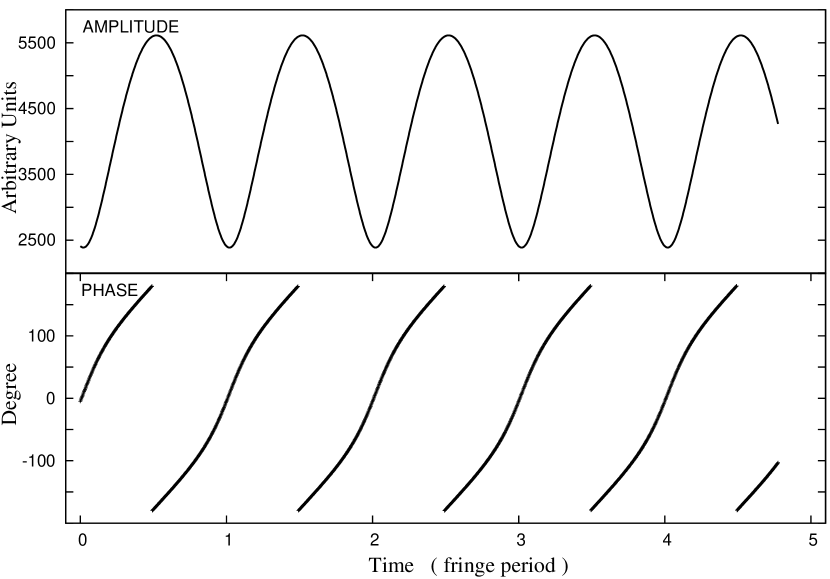
Figure 2: Observed visibility in the presence of RFI for the model shown in Fig. 1. The amplitude and phase, derived from Eqn 2 are plotted against time. The observed data may be fit by well-defined analytical expressions to estimate the contribution of RFI to the observed visibility.

where, all terms are complex, $\mathcal{A}$ and $\Phi$ are the amplitude and phase of the RFI in the baseline and $\nu_{{}_{F}}$ is the fringe-stop frequency (Eqn. 1). Provided the RFI remains constant over a good fraction of the fringe period, the observed data may be fitted for fit-average values of $\mathcal{A}$, $\Phi$, and $V_{{}_{TRUE}}$. The observed visibility amplitude and phase obtained in a closed/analytical form from Eqn. 2 are plotted in Fig. 2. The salvaged/RFI-free visibility will then be

$$V^{j}_{{}_{RFIX}}=V^{j}_{{}_{OBS}}-\mathcal{A}e^{i[{2\pi\nu_{{}_{F}}(t)}t^{j}-\Phi]}\equiv V_{{}_{TRUE}}+Noise^{j}$$ (3)

where, $j$ is an index identifying a particular data point in the subset over which the RFI was presumed to be constant and a model was fit. Note that $V_{{}_{TRUE}}$, $\mathcal{A}$ and $\Phi$ do not carry the index $j$ and are average fit values for the entire subset. The average $V_{{}_{TRUE}}$ obtained from the fit is not carried to the next stage. Instead, the model RFI contribution ($\mathcal{A}$ and $\Phi$) for the fitted subset is subtracted from the j-th observed visibility (within the subset) to obtain the j-th modified visibility; i.e. the modified values continue to carry the original unsmoothed noise component and hence adjacent values remain independent.

This technique does not affect the all-important closure relationships (Thomson et al., 1986). The mean value of $V_{{}_{OBS}}$ (i.e. the centre of the circle) is a good estimator of $V_{{}_{TRUE}}$ and can be used to quantify deviations from closure, if any. Alternatively, one can consider the case of an inaccurate estimate of the RFI amplitude and phase. Since the modified visibilities are obtained by subtracting the RFI circle, an inaccurate RFI model is equivalent to the original RFI corruption being replaced by a new RFI corruption, whose amplitude should be close to zero under ideal conditions but in any case smaller than the original RFI amplitude. In practice, a simple before-and-after rms calculation and $\langle V_{{}_{RFIX}}\rangle-\langle V_{{}_{OBS}}\rangle$ can be used to quantify closure deviations, if any, and provide the choice of either using the model fit or retaining the original data — at worst the processed data is no worse than the raw data.

The relative strengths of the RFI and true visibility is not relevant either since the algorithm is being applied on the rectilinear complex plane.

3 Implementation at GMRT — RfiX package

The RFI environment at GMRT can be quite intimidating, especially at frequencies below 400 MHz. While the strongest source in a field is typically only a few Jy, the RFI can occasionally reach several hundred Jy in some channels in the 150 and 240 MHz bands.

However broadband RFI of up to several tens of Jy causes even more damage: currently available tools, including the Astronomical Image Processing System (AIPS) and FLAGIT (a locally developed tool) would not even recognise the RFI contamination — there is no ”clean” reference area for identification by contrast.

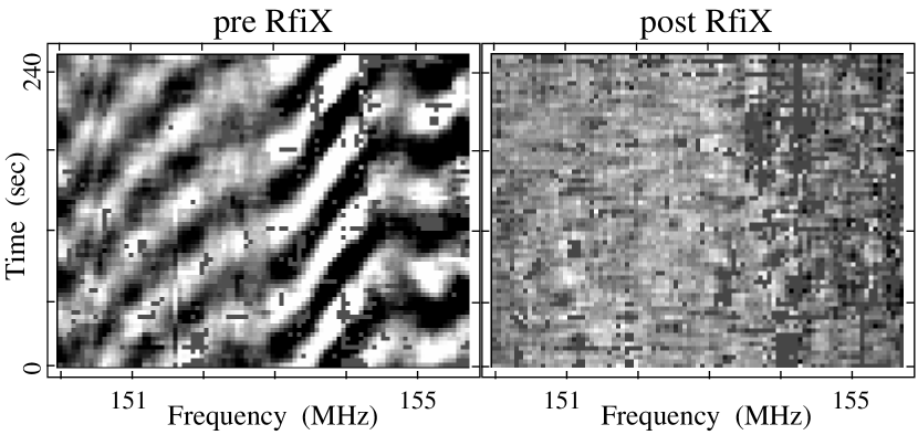
Figure 3: Pre- and post-RfiX views of the visibility Time-Channel plane. Each pixel is 4.18 second in time and 62.5 KHz in frequency. Every single channel is afflicted by RFI and each different gradiant seen on the left panel represents a different RFI source. Application of RfiX results in a more-or-less featureless, i.e. RFI-free, plane (right). RfiX does not require clean reference areas to eliminate RFI.

This may be seen in Fig. 3 which plots the visibilities in grey-scale on a 2-dimensional time-frequency plot. In the absence of RFI all the visibilities in a small subsection of the time-frequency plane should more-or-less represent the same fourier component for a continuum source and hence the intensity pattern should be devoid of features. A very narrow RFI line would show up as a ripple along the time axis in a single frequency channel. A coherent broad-band RFI source would introduce a ripple across many channels and the direction of the pattern would depend on the location of the RFI with respect to the baseline. The ripples seen in the left-hand panel show that the visibility data shown has RFI in every single time-frequency pixel. The different slopes seen in the pattern points to the presence of multiple sources of RFI which have emission broad enough to cover many channels (of up to several MHz) but not broad enough to cover the whole band, which complicates data analysis as will be described shortly.

Broadband RFI causes calibration errors which severely limit the dynamic range (Peak-to-rms ratio) to less than a few thousand at these frequencies, even for observations of several full synthesis sessions (each of 8-10 hours). Even though the GMRT is currently the most sensitive low frequency instrument the sensitivity achieved at 150 and 240 MHz is more than a factor of 10 poorer than expected for long integrations.

There are two ways of removing RFI from the data. A fourier transform of the time-frequency visibility data would efficiently localise the RFI signal in frequency-lag space (time-lag $\equiv$ path difference from the RFI source to the 2 antennas). A fourier transform requires many dozens or even hundreds of data points within the period of constancy of the RFI source for efficient inversion. This requires higher (than usual) speed sampling and storage for consequent larger data volume. Furthermore, abrupt changes along either the time- or the frequency-axis, like the ones seen in Fig. 3, will make the frequency-lag plane noisier, reducing the ability to detect RFI.

The alternative chosen for RfiX was motivated by the realisation that while RFI ripples along the frequency axis could have different scale-lengths they would all have exactly the same period along the time axis and this period was identical to the analytically defined fringe-stop period used by the correlator. The RFI in each channel was estimated independently by fitting a 1-dim sinusoid in time (instead of a 2-dim fourier transform), which has several advantages: (i) it eliminates all modulation scales other than the fringe-stop period from the analysis; fitting a single sinusoid of known period is a simple linear process with well-defined error estimates, (ii) it affords greater flexibility and efficiency in identifying the time subsections of constancy of RFI in each channel, thus accommodating the abrupt changes in the time-frequency plane seen in Fig. 3, and (iii) since the model only has 4 free parameters and the sinusoid period is fixed one can safely restrict the fitting process to small data sections and hence greater chance of constancy of RFI and more accurate RFI excision.

While the standard mode of the GMRT correlator outputs visibilities every 16.7s one can also trivially select faster data output modes which provide visibilities every 2 or 4, and exceptionally even 0.128, seconds. Recording the data every $2-4$ seconds is sufficient for this algorithm; one should compare this to the nano- to millisecond sampling rate usually required by most other techniques of RFI removal. Using data integrated for several seconds has the advantage of (i) not requiring additional hardware (ii) easily manageable data output rate and hence (iii) the option of offline processing. Additionally, this longish integration time reduced the measurement noise in each visibility and allowed for detection and excision of fainter RFI.

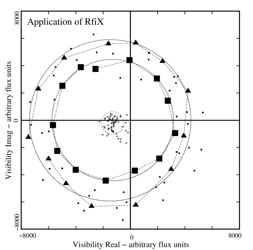
Figure 4: RfiX algorithm, applied to the observed data plotted in Fig. 1. The outer annulus of points (large squares, triangles and dots) is the raw data from a 5-minute GMRT scan at 153 MHz. The two subsets of 13 data points (large squares and triangles) connected by dashed lines are two temporal sequences spanning one fringe period each and the solid circle associated with each is the model fringe due to RFI. The other subsets and their fits have been omitted for clarity. The inner cluster of points are the modified (true) visibilities obtained by subtracting the model fringe from the raw visibilities. The small dashed circle around the inner cluster denotes the 3$\sigma$ of the scatter.

Figure 4 illustrates the application of the algorithm to actual data. The plot shows a 5 minute data sequence from a single channel (same as in Fig. 1). The outer annulus of points is the raw data. The compact cluster at the centre is the processed/RFI excised data. The variability of RFI within the 5 minute scan was surmounted by separate fits to subsets of the data of length 54s (= 1 fringe period). Nevertheless, this variability resulted in imperfect RFI mitigation, which is reflected in a larger scatter in the modified visibilites. However, RfiX succeeded in reducing the scatter by a factor of 5, from the radius of the outer annulus (RFI amplitude) to the post-processing scatter represented by the small inner circle. This much smaller scatter facilitates further cleaning-up through sigma-clipping.

The fully automated implementation: (i) checks if the baseline fringe-stop period is within the appropriate range (see under Discussion) and if not, either skips it or flags it as specified (ii) compares the scan rms to a fiducial value to determine if the particular channel has significant quantum of RFI and therefore worth processing, (iii) identifies subsections with constant RFI amplitude and (iv) robustly fits and subtracts the RFI fringe

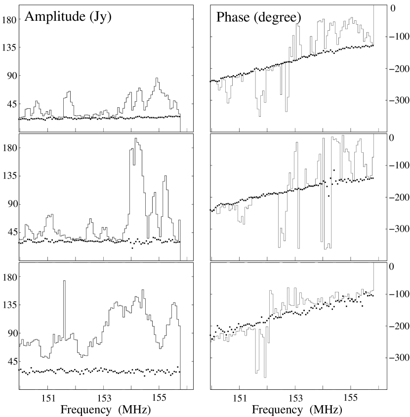
Figure 5: Efficacy of RfiX in cleaning the bandpass. The panels show the average bandpass for three 5-minute scans spanning a 4-hr period of the strong calibrator 3C446 at 153 MHz using the GMRT. The solid histograms are the pre-RfiX (raw) data and the dots are the post-RfiX visibilities. The source flux density is 21.5 Jy. The strongest RFI (middle scan) is almost 200 Jy. The bottom scan has at least 25 Jy of RFI in every channel and four times as much in some. In spite of the very strong RFI the post-RfiX bandpass is more or less flat in amplitude and linear in phase and the amplitude level and phase gradient is similar in all 3 scans.

Figure 5 shows the results of RfiX on the averaged bandpass of amplitude and phase of three different 5-minute scans (separated by 4 hours). The data was obtained with the GMRT at 153 MHz on the calibrator source 3C446 (21.5 Jy). The upper panel shows RFI nudging 200 Jy in some channels. The lowermost panel is a remarkable example of the algorithm’s efficacy. The entire band is corrupted by at least 25 Jy of RFI, with even larger contamination in some channels. Traditional methods of offline RFI clipping (in AIPS, for instance) would completely fail in this case. The large amplitude bias would have cascaded across the data during self-calibration, vitiating the gain solutions of all antennas including those without RFI. While this is an extreme example it happens often enough to seriously limit the sensitivity at 130-250 MHz. Even though each frequency channel in each scan was processed independently and the RFI varied considerably the amplitude is more-or-less flat across the band and from scan to scan, as also the phase gradient across the band. This is good evidence that the algorithm is not corrupting the closure quantities.

Figure 3 shows the visibility time-channel plot of a scan and the efficacy of RfiX even when every single channel and time is affected by strong RFI.

Figure 6 shows an image of the 3C286 field from 2 hours of GMRT observations at 240 MHz. 3C286 is 28 Jy at that frequency. The rms noise at the centre of the field (close to 3C286) is 2 mJy/beam ($Peak/noise\sim 14000$). Furthermore, despite the very strong source the central region is mostly clean with only one artifact reaching 8$\sigma$. The noise at the periphery is only 0.65 mJy/beam ($Peak/noise\sim 14000$). Histograms of the noise pixels show that the image is ”clean” with no residuals in excess of 4$\sigma$. This is perhaps the highest dynamic range image achieved till date at frequencies below 300 MHz (wavelength $>$1m).

4 Discussion

The most important feature of RfiX is its ability to salvage RFI-corrupted data — it not only identifies RFI but also excises it to obtain uncorrupted data. This is perhaps the only RFI mitigation tool which is entirely software based. It can be applied offline on the normal correlator data typically output every $0.1-30$ seconds. This much longer integration compared to high-speed sampling techniques makes RfiX sensitive to fainter RFI. It complements high-speed techniques which are best for clipping short but intense bursts of RFI but cannot target weak but constantly present RFI. Also, RfiX does not require a clean reference area to identify RFI.

The technique is applicable to any interferometer which uses fringe-stopping. It can also be applied at any frequency provided only that the correlator output matches the Nyquist rate for the fringe-stop frequency of the particular baseline. For instance, the GMRT correlator outputs data every 2-16 seconds in the standard mode. A 2s sampling rate limits the application of RfiX to baselines with $U_{\lambda}<3-12k\lambda$ (declination range $0^{o}-75^{o}$). At the GMRT the RFI is most severe at $\nu_{OBS}<400$ MHz and at these frequencies the above limit corresponds to baselines of several kilometres. We do not usually find correlated RFI on such long baselines and so the sampling rate does not pose a constraint in practical terms. In any case, the present correlator at GMRT can be configured to provide data every 0.128 second and so, if necessary, the longer baselines and/or higher frequency observations can also be processed for RFI using RfiX. In general, a visibility sampling interval of 0.1s, which can be very easily achieved using present-day hardware, will be sufficient for excising RFI (using RfiX) from baselines up to a few km in observations up to a few GHz. Of course, shorter visibility integrations in the correlator can relax both these limits.

RfiX will not work effectively with interferometric observations near the Celestial Poles where the fringe rate is very slow. Even in regions away from the Poles baselines with small $U$-component (see Eqn. 1) have very long fringe periods and so cannot be satisfactorily processed. RfiX works best for RFI which manifests and remains constant over the fringe period of a baseline. Fitting over a full fringe period is very safe for conserving closure. Fitting intervals shorter than a third of the fringe period could lead to incorrect estimation of RFI amplitude and hence closure-violating baseline errors. At the GMRT the RFI amplitude can be quasi-constant for up to 150-200 seconds which limits the application of RfiX to baselines with fringe periods $\leq 500$ seconds, corresponding to baseline component $U_{\lambda}$ $\geq 25-100\lambda$ (declination range $0^{o}-75^{o}$). Of course, we do see instances of RFI varying on much shorter timescales and RfiX will fail in those cases. Depending on the goal one can either flag all shorter baselines or retain them without RfiX processing. Therefore, this algorithm will not improve the quality of image structures larger than $0.^{\rm{o}}5-1.^{\rm{o}}5$. This is not a serious limitation since the GMRT primary beam FWHM is not much larger. Note that the constraint comes from the timescale of RFI variability and not RfiX. Pen et al. (2008) also have a similar limitation for excising RFI in baselines with long fringe periods.

Briefly, the limiting fringe stopping frequency and the corresponding baseline for which RfiX is effective are related through the rather simple Equation 1. It must be noted that only the baseline component $U_{\lambda}$ is involved in the equation and not $V_{\lambda}$. The lower baseline limit is defined by the timescale of RFI variability while the upper limit is set by the visibility integration period of the correlator.

It is often claimed that interferometric fringe-stopping in itself washes out RFI, but this is not entirely appropriate for low frequency arrays. If the system temperature (T_sys) dominates over the RFI amplitude (A_RFI) the noise in a single visibility of integration period $\tau$ will be T${}_{sys}/\sqrt{\tau}$. When RFI dominates the effective noise will be A${}_{\rm{RFI}}/(\nu_{{}_{F}}\tau)$, where $\nu_{{}_{F}}$ is the fringe-stop frequency for the particular baseline. Thus, RFI suppression due to fringe-stopping is most effective for short baselines for which $\nu_{{}_{F}}\tau\gg 1$. In the context of GMRT observations at 153 MHz (longest baseline 27 km) the shortest fringe period is of the order 1 second (see Eqn. 1) compared to the recommended integration time of 2-4 seconds. Therefore RFI suppression due to fringe stopping would only have a marginal impact. Even at 1 GHz RFI would be suppressed only in baselines formed by the outer antennas; but correlated RFI is anyway mostly limited to baselines shorter than a few km. RFI suppression due to fringe-stopping would be most effective in arrays operating at $\nu\gg 1$ GHz as even the shorter (RFI-prone) baselines will have sufficiently short fringe period to achieve RFI suppression.

A detailed description of the implementation of RfiX for GMRT data is presented in (Athreya, 2009) and may be of use to astronomers intending to implement the tool at other facilities.

RfiX is somewhat related to the RFI-to-North-Pole scheme tried by Perley et al. (2005). Briefly, a stationary RFI and a source at the North-Pole are both stationary with respect to the interferometer. Thus, one can attempt to map RFI to pseudo sources at the North Pole and subtract them from visbilities. This will work when the RFI contributes the same antenna temperature to all the antennas, just like a celestial source. However, in general the intensity of an RFI source varies from antenna to antenna due to $1/R^{2}$ fall-off and shielding by manmade or geographical structures. RfiX surmounts this problem by processing each baseline separately allowing for variable intensity in each.

In summary, RfiX is a powerful tool based on a simple concept for mitigating RFI in interferometric data. Indeed, its strength lies in its simplicity which provides a clear understanding of its domain of applicability. It not only identifies RFI but also salvages RFI-affected visibilities. It is a purely software approach which requires neither additional hardware, nor real-time analysis nor complicated mathematical operations and can even be applied to archival data. It complements other extant excision techniques in approach and domain of applicability. It will work for any interferometer which uses fringe-stopping.

Figure 1: Effect of fringe-stopping and stationary RFI on the true visibility. The rectilinear complex-plane plots (not to be confused with the UV plane) show the temporal behaviour of the true and observed values of the visibility from a single baseline. Left: schematic illustration — fringe-stopping causes the RFI (dashed vector) to circulate around the true visibility (solid vector) at the fringe-stop frequency for the baseline. The resultant amplitude (dotted vectors) and phase (their position angle w.r.t Real-axis) vary with time in an analytically calculable manner (see Fig. 2). Right: actual data — 5 minute sequence of GMRT 153 MHz data from C00-C04 baseline exhibiting the visibility circulation. Adjacent points along the curve are separated by 4.18 second.

Figure 6: GMRT image of 3C286 at 240 MHz using RfiX processed data. The left panels show the celestial sources (top) and the rms noise (bottom), respectively. They were made using just 2 hours of data with the GMRT. The field covers the half-power extent of the primary beam. The peak flux density is 28 Jy (of 3C286) and the noise is 2 mJy/beam near 3C286 and 0.65 mJy/beam at the periphery ($Peak/noise\equiv$ centre: 14000, periphery: 43000). This is perhaps the highest dynamic range image made at wavelength $>$ 1m (frequency $<$ 300 MHz). The plot illustrates, rather starkly, the problem of finding isolated point sources for calibration at low frequencies! The top-row middle panel shows a more detailed plot of the immediate area around 3C286. As may be expected artifacts are most numerous here, but even so the image is quite clean with only few artifacts in excess of $5\sigma$, with the highest at $8\sigma$. In the peripheral regions (top-right) there are no artifacts in excess of $4\sigma$. Histograms of the noise pixels (bottom row) near the contour locations show well-behaved residuals.

References

- Athreya (2009) Athreya, R. M. 2009, National Centre for Radio Astrophysics Tech. Report, in prep.
- Baan et al. (2004) Baan, W. A., Fridman, P. A., Millenaar, R. P. 2004, AJ, 128, 933
- Bhat et al (2005) Bhat, N.D.R., Cordes, J.M., Chatterjee, S., Lazio, T.J.W. 2005, Radio Science, 40(5) (arXiv:astro-ph/0502149v1)
- Boonstra & van der Tol (2005) Boonstra, A. J., van der Tol, S. 2005, Proc of the RFI2004 workshop, Radio Science, 40
- Bradley & Barnbaum (1998) Bradley, R., Barnbaum, C. 1998, AJ, 116, 2598
- Briggs et al. (2000) Briggs, F. H., Bell, J. F., Kesteven, M. J. 2000, AJ, 120, 3351
- Ellingson et al. (2001) Ellingson, S. W., Bunton, J. D., Bell, J. F. 2001, ApJS, 135, 87–93.
- Fridman (2001) Fridman, P.A.: 2001, å, 368, 369
- Fridman (2008) Fridman, P.A.: 2008, AJ, 135, 1810
- Kocz (2004) Kocz, J. 2004, Radio frequency interference characterisation and excision in radio astronomy, Honours thesis, Dept of Engineering, The Australian National University.
- Lesham et al. (2000) Leshem, A., van der Veen, A. J., Boonstra A. J. 2000, ApJS, 131, 355
- Pen et al. (2008) Pen, U.-L., Chang, T.-C., Peterson, J. B., Roy, J., Gupta, Y., Bandura, K. 2008, arXiv:astro-ph/0804.2501v1
- Perley et al. (2005) Perley, R. A., Cornwell, T. J., Bhatnagar, S., Golap, K. 2005, Proc of the RFI2004 workshop, Radio Science, 40
- Thomson et al. (1986) Thomson, A. R., Moran, J. M., & Swenson G. W. 1986, Interferometry and Synthesis in Radio Astronomy (Wiley Interscience, New York).
- Winkel et al. (2007) Winkel, B., Kerp, J., & Stanko S. 2007, Astron. Nachr., 328, 68